THE MIXING APPROACH AS A UNIFYING FRAMEWORK FOR ...

THE MIXING APPROACH AS A UNIFYING FRAMEWORK FOR DYNAMIC MULTIVARIATE ANALYSIS JAN DE LEEUW, CATRIEN BIJLEVELD, KEES VAN MONTFORT, AND FRITS BIJLEVELD Abstract

We argue that many models for multivariate longitudinal and cross-sectional data analysis have a common ancestry. They all are based on the qualitative idea that if we knew the actual state of the world, the relations between the observed quantities would be truly simple. This is shown to lead directly to factor analysis, IRT, state space models, mixture densities, latent Markov chains, MIMIC, LISREL, and various other common models and techniques. We show how our approach provides a convenient framework for looking at these models. The EM algorithm can be used to estimate the unknown parameters. An additional advantage of our approach is that it can incorporate continuous as well as interval, ordinal and categorical variables .

1. Introduction Our starting point in this paper is that we want to describe the relationships between (possibly many) variables, and we want to describe this relationship in simple terms. We look for simplicity, not necessarily because we believe the world is simple, but because simple relationships are easier to manipulate and communicate. For Quetelet, Galton, and the early Karl Pearson, the normal distribution was simple. When Pearson [18] rst came across non-normal variation in his biometric work, he tried to maintain this notion of simplicity by assuming that the sample came from a mixture of normal distributions. Thus normality was still the norm, but unfortunately the sample was impure, because it consisted of a mixture of types. If we could have Date : November 19, 1996. Catrien Bijleveld Department of Research Methodology and Psychometrics University of Leiden P.O. BOX 9555 2300 RB Leiden the Netherlands 1

.

2 JAN DE LEEUW, CATRIEN BIJLEVELD, KEES VAN MONTFORT, AND FRITS BIJLEVELD

separated the types by observation, we would have seen the normality, but because we couldn't the statistical analysis has to do the job instead. In the same way, the Pearson polychoric model is based on the notion that multivariate normal is simple. Unfortunately we can only observe discreticized versions of the variables, which means we observe multinormals \mixed" over cell contents. In the same way for Spearman [19], intelligence was simple. It was a construct very much like the weight of an object, and the test was like a spring balance. It was a construct much like the weight of an object, and the test was the spring balance. If wi is the weight of object i, and aj is the resistance of spring j, then Hooke's Law tells us that the extension of the spring is yij = wiaj . This is basically Spearman's model. Score on the test was proportional to the \weight" of the subject and to the \resistance" of the test. All other relationships between the tests, if they were indeed proper tests of intelligence, were measurement errors, i.e. they were dictated by chance. If we select a population of persons with a xed intelligence, then the tests will be perfectly uncorrelated. Correlation between tests is merely a consequence of the fact that we cannot select such \pure" populations, i.e. it is a consequence of the fact that our populations are of mixed intelligence. If we knew the \state" of the system, i.e. the person's intelligence, then the correlation would disappear. This very same idea comes back in Lazarsfeld's [13] latent class analysis, in a very simple discrete form. It also has dominated item analysis, or item response theory, ever since the work of Lawley [12]. In item response theory the basic assumption is called local independence, and the relationship between the variables is \explained" by mixing populations with local independence. Factor analysis, latent class analysis, and item response theory are all special cases of the analysis of inter-dependence. All variables play the same symmetric role in the model, we do not measure any input to the system, only output. In the analysis of dependence, it is precisely the relationship between input and output variables that we are interested in, and the model is inherently asymmetric because of this. In classical regression analysis there is a very simple model for each cell in the design. All cells corresponds with normal distributions with the same shape, with a cell-speci c shift. The joint distribution of the predictors and the outcome is a mixture of the cell distributions, although in this case the mixing proportions are known. By using the design matrix, we automatically unmix the distribution. The mixing variable is completely known, and thus we can analyze conditionally on its values (we consider the design matrix as xed and known). The notion of local independence is applied most naturally in the analysis of dependence by using MIMIC models. MIMIC models, introduced by Joreskog and Goldberger [10],

THE MIXING APPROACH FOR DYNAMIC MULTIVARIATE ANALYSIS

3

again revolve the notion of a state, similar to intelligence or ability. Within a given state, input and output are independent. Or, to put it dierently, the state splits input and output, and all in uence of the input on the output goes through the state. States are unobserved, as usual, and dependence of input on output comes about by mixing states. MIMIC notions are easy to generalize to the longitudinal situation, in which we observe the same input-output system at various points in time. This de nes a sequence of MIMIC models. Of course replicating a MIMIC model on independent individuals also leads to a sequence of MIMIC models, but in that case the models are unconnected, because of independence. In the case of temporal variation, we need to connect the models because of the time-dependence. The basic idea in dynamic multivariate analysis is to link the models through the state variables. Not only do the state variables split input and output, they also split points in time. Thus all information about the past is collected in the present state of the system, and if we knew the present state, our predictions would not be improved by knowing about the past. Given the present state, we agree with Henry Ford that \history is bunk". In the next section we will make these notions more precise, but for the time being it suces to observe that Joreskog and Goldberger's marriage of factor analysis and regression analysis can be extended in the time dimension to include state space analysis. In time, we have linked MIMIC models, and these linked MIMIC models may be stacked on top of each other if we have independent replications. We are interested in the time evolution of the state, because that summarizes all the relevant information for prediction, and thus all the relevant dynamics in the system. If state in cross-sectional factor analysis is intelligence, then state in state space models in the same context is development of intelligence, with similar interpretations for ability. It is of importance to emphasize that in cross-sectional latent variable theory, a great deal has been made out of the fact that input, output, and state can all be either discrete or continuous. Regression of output on state can have many dierent possible forms because of this reason. The basic notion of state, or of latent variables, or of conditional independence, is not related to the nature of the various regressions, which should be tailored to the problem at hand.

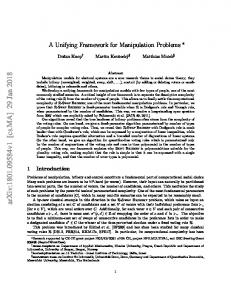
2. Dynamic Multivariate Models The basic model we are interested in is drawn in Figure 1. Actually there are N such models, one for each individual. The individuals are independent. We write

4 JAN DE LEEUW, CATRIEN BIJLEVELD, KEES VAN MONTFORT, AND FRITS BIJLEVELD

x

z

i0

z

i1

i1

y i1

x

x

i2

...

z

i2

y i2

z

iT

iT

y iT

Figure 1. Linear dynamic model for individual i.

(2.1)

prob[(^Ni=1 ^Tt=1 yit )(^Ni=1 ^Tt=0 zit )(^Ni=1 ^Tt=1 xit )]

for the probability of observing the data X , Y and Z . Our basic task in this section is to derive a general expression for this probability, taking the properties of the model in Figure 1 into account. The key result used to translate directed acyclic graphs into statements about joint distributions is a simple one. We suppose that, given zit , yit is independent of all other variables. Also, given zi;t?1 and xit ; zit is independent of all other variables. Under these conditions theorem 2.1 is valid.

Theorem 2.1. prob[(^Tt=1 yit )(^Tt=0 zit )(^Tt=1 xit )] = prob[^Tt=1 xit j zi0 ]prob[zi0 ]

YT t=1

prob[yit j zit ]prob[zit j zi;t?1 ^ xi;t ]

Proof. The proof is by induction over T: The result is trivially true for T = 1: Assume it is true for T ? 1: Start with a simple application of the de nition of conditional probability.

THE MIXING APPROACH FOR DYNAMIC MULTIVARIATE ANALYSIS

5

prob[(^Tt=1 yit)(^Tt=0 zit )(^Tt=1 xit )] = prob[yiT j (^Tt=1?1 yit)(^Tt=0 zit )(^Tt=1 xit )]  prob[ziT j (^Tt=1?1 yit)(^Tt=0?1zit )(^Tt=1 xit )]  prob[xiT j (^Tt=1?1yit)(^Tt=0?1 zit )(^Tt=1?1xit )]  prob[(^Tt=1?1 yit)(^Tt=0?1 zit )(^Tt=1?1xit )] The assumption about yit, zit and xit tells us prob[yiT j (^Tt=1?1yit )(^Tt=0 zit )(^Tt=1 xit )] = prob[yiT j ziT ]; and prob[ziT j (^Tt=1?1yit )(^Tt=0?1zit )(^Tt=1 xit )] = prob[ziT j zi;T ?1 ^ xi;T ]; and prob[xiT j (^Tt=1?1yit )(^Tt=0?1zit )(^Tt=1?1 xit )] = prob[xiT j ^Tt=1?1xit ^ zi0 ]: But this means that we have proved the recursion prob[(^Tt=1 yit)(^Tt=0 zit )(^Tt=1 xit )] = prob[yiT j ziT ]prob[ziT j zi;T ?1 ^ xi;T ]prob[xiT j ^Tt=1?1xit ^ zi0 ] prob[(^Tt=1?1 yit)(^Tt=0?1 zit )(^Tt=1?1xit )]: By the induction hypothesis this means the result is true for T: We now introduce some simplifying assumptions, which just serve to make the nal result easier to write down. If necessary, they can be gotten rid of again.

Corollary 2.2. If prob[^Tt=1 xit j zi0 ] = prob[^Tt=1 xit ] and zi0 is a.s. equal to 0, then

6 JAN DE LEEUW, CATRIEN BIJLEVELD, KEES VAN MONTFORT, AND FRITS BIJLEVELD

prob[^Tt=1 yit j ^Tt=1 xit ] =

Z






Z

YT z 0 ;:::;z t=1 i

prob[yit j zit ]prob[zit j zi;t?1 ^ xi;t ]dziT : : : dzi0 :

iT

Proof. Start with the result in Theorem 2.1. We remove the marginal distribution of the input variables by conditioning, and then integrate out the state variables.

We see that the latent variables or state variables serve two purposes. They mediate the eect of input on output, and they channel the eect of the past on the present. Actually, the state space process is rst-order Markov, although the observed output process can be much more complicated. The rst-order Markov property is the basic notion of simplicity used in this context. It is clear that the state variables, with their double function, have to do a lot of work, and consequently the dimensionality of the state space (the \number of factors") may have to be quite big for a satisfactory t. 3. Specific Submodels There are a number of useful distinctions that can be drawn in discussing this class of models. In the rst place there are models with and without input. There are models in which the state variables are discrete, and models in which they are continuous. In some models the input and/or output variables are discrete, in others continuous. There are models which are cross-sectional, in the sense that T = 1; and models which are time-series, in the sense that N = 1: Discussing the models in these terms shows that they do indeed cover a lot of the latent variable models discussed in psychometrics and other disciplines. We shall discuss a number of these special cases in a little bit more detail. What we propose here is a simple and straightforward widening of the framework introduced by Lazarsfeld [13] and Guttman [8] in the forties, and then extended by Anderson [1], McDonald [15], and Bartholomew [2] for cross-sectional models, and of the framework discussed, for example, by Metz [16] for time series. As mentioned in the introduction, in the class of cross-sectional models without input we nd factor analysis (continuous state, continuous output), latent class analysis (discrete state, discrete output), latent pro le analysis (discrete state, continuous output), latent trait analysis (continuous state, discrete output), and of course various combinations of these techniques. MIMIC models are cross-sectional with input, and again we can have discrete/continuous state-space and discrete/continuous input/output to

THE MIXING APPROACH FOR DYNAMIC MULTIVARIATE ANALYSIS

7

describe various MIMIC variations. Classical state space models are usually for the time-series situation, in which N = 1, although this is by no means necessary. If N = 1 the state space model does have far too many parameters, and we need to get statistical stability from additional assumptions. The obvious one is stationarity, which means that the \structural" parameters of the model are constant over time. In this way observing more time points gives us more information about these parameters, and thus, in the limit, they can be estimated consistently. If N >> 1 we can hope to estimate nonstationary models, such as the discrete latent Markov chains discussed by Van der Pol and De Leeuw [20], or the continuous LISREL-type models discussed by MacCallum and Ashby [14] and Oud [17]. There is an elegant device, familiar from the psychometric tradition, but actually starting with Pearson, which makes it possible to generate models with discrete (or truncated, or transformed) output from models with continuous output. This can be translated in terms of simplicity. We think the continuous models are simple, and we build models for the observed variables on the basis of these simple models. Before we discuss these, we shall look at continuous models in more detail. 4. Continuous output variables Models with continuous variables remain important, because they are parsimonious, and because they can be used as stepping stones to construct models with continuous latent indicators. The previous formulations of the model were given in terms of the density or probability mass function. Now we will introduce model parameters and will switch to the equivalent formulation in terms of random variables, which we distinguish from xed quantities by underlining. The conditional expected value and variance of the output given the input are computed. The natural assumptions in this case are linearity of regression and homoscedasticity. We look at the equations for a xed value of i: More precisely, we assume that the conditional expectation of yt given ^ts=0 z s and ^ts=1xs depends linearly on z t only. Moreover, the conditional expectation of z t given ^ts?=01 zs and ^ts=1xs depends on z t?1 and xt only. Thus (4.1a) (4.1b) where

y t = Ht z t +  t ; z t = Ft zt?1 + Gt xt + t ;

8 JAN DE LEEUW, CATRIEN BIJLEVELD, KEES VAN MONTFORT, AND FRITS BIJLEVELD

t ? ^ts=0 z s; t ? ^ts=1 xs; t ? ^ts?=01 z s; t ? ^ts=1 xs; and homoscedasticity means

V (t ) = ; V (t ) = : These equations de ne the discrete linear system, made famous by Kalman. In these classical state space models it is usually assumed that the matrices Ft ; Gt and Ht (and even and ) are known from the physics of the problem, and only the state variables have to be estimated. For this the Kalman lter is applied, which is in this sense a method for computing \factor scores".

Lemma 4.1.

t ? ^ts=1 s; t ? ^ts?=11 s:

Proof. Again we use recursion.

Theorem 4.2. Suppose, again to simplify notation, that z i0 is a.s. equal to zero. We de ne

8Qt < k=s+1 Fk Pts = : I

s