the performance of clustering approach with robust

THE PERFORMANCE OF CLUSTERING APPROACH WITH ROBUST MM-ESTIMATOR

15

Jurnal Teknologi, 45(C) Dis 2006: 15–28 © Universiti Teknologi Malaysia

THE PERFORMANCE OF CLUSTERING APPROACH WITH ROBUST MM-ESTIMATOR FOR MULTIPLE OUTLIER DETECTION IN LINEAR REGRESSION NURULHUDA FIRDAUS MOHD AZMI1, HABSHAH MIDI2 & NORANITA FAIRUS ISMAIL3 Abstract. Identifying outlier is a fundamental step in the regression model building process. Outlying observations should be identified because of their potential effect on the fitted model. As a result of the need to identify outliers, numerous outlying measures such as residuals and hat matrix diagonal are built. However, these outlying measures works well when a regression data set contains only a single outlying point and it is well established that regression real data sets may have multiple outlying observations that individually are not easy to identify by the same measures. In this paper, an alternative approach is proposed, that is clustering technique incorporated with robust estimator for multiple outlier identification. The robust estimator proposes is MM-Estimator. The performance of clustering approach with proposed estimator is compared with other estimator that is the classical estimator namely Least Square (LS) and other robust estimator that is Least Trimmed Square (LTS). The evaluation of the estimator performance is carried out through analyses on a classical multiple outlier data sets found in the literature and simulated multiple outlier data sets. Additionally, the analysis of Root Mean Square Error (RMSE) value and coverage probabilities of Bootstrap Bias Corrected and Accelerated (BCa) confidence interval are also being conducted to identify the best estimator in identification of multiple outliers. From the analysis, it has been revealed that the MMEstimator performed excellently on the classical multiple outlier data sets and a wide variety of simulated data sets with any percentage of outliers, any number of regressor variables and any sample sizes followed by LTS and LS. The analysis also showed that the value of RMSE of the proposed estimator is always smaller than the other two estimators. Whereupon, the coverage probabilities of BCa confidence interval also conclude that the MM-Estimator confidence interval have all the criteria’s to be the best estimator since it has a good coverage probabilities, good equatailness and the shortest average confident length followed by LTS and LS. Keywords: Multiple outliers, linear regression, robust estimator, MM-Estimator, Bootstrap Bias Corrected and Accelerated (BCa) confidence interval Abstrak. Pengenalpastian cerapan data yang terpencil daripada kelompok cerapan merupakan langkah asas dalam membina model regresi. Oleh kerana cerapan data yang terpencil ini memberi kesan kepada model yang dibangunkan, pelbagai ukuran terhadap pengenalpastian cerapan data yang terpencil telah dibina. Sebagai contoh, ukuran residual dan ukuran matrik identiti bagi hat matrix. 1 2 3

Centre for Advanced Software Engineering (CASE), Universiti Teknologi Malaysia City Campus, Jalan Semarak, 54100 Kuala Lumpur, Malaysia. Email: [email protected] Institut Penyelidikan Matematik (INSPEM), Universiti Putra Malaysia, 43400 UPM Serdang, Selangor Darul Ehsan, Malaysia. Email: [email protected] Fakulti Sains Komputer & Sistem Maklumat, Universiti Teknologi Malaysia, 81310 UTM Skudai, Johor Darul Ta’zim, Malaysia. Email: [email protected]

JTDIS45C[B]new.pmd

15

01/13/2009, 09:55

16

NURULHUDA FIRDAUS, HABSHAH, & NORANITA FAIRUS Walau bagaimanapun, ukuran-ukuran ini hanya dapat mengukur dengan baik jika di dalam set data itu terkandung hanya satu atau sedikit cerapan data yang terpencil, walhal jika data dicerap berdasarkan kepada persekitaran sebenar berkemungkinan terdapat lebih banyak cerapan data yang terpencil. Kertas kerja ini mencadangkan pendekatan alternatif iaitu penggunaan teknik kelompok bersama penganggar statistik tegap di dalam pengenalpastian kumpulan cerapan data terpencil. Penganggar statistik tegap yang dicadangkan ialah penganggar MM. Penilaian terhadap kebolehupayaan pendekatan kelompok bersama penganggar cadangan, diuji melalui perbandingan dengan penganggar klasik Least Square (LS) dan penganggar statistik tegap yang lain iaitu Least Trimmed Square (LTS). Pengujian dilakukan melalui analisis pada kumpulan set data terpencil klasik yang diperolehi daripada kajian literatur dan kumpulan set data yang diperolehi daripada simulasi. Sebagai tambahan, kebolehupayaan bagi ketiga-tiga penganggar ini seterusnya diuji berdasarkan nilai punca kuasa dua ralat (RMSE) dan kebarangkalian liputan bagi selang keyakinan Bootstrap Bias Corrected and Accelerated (BCa) bagi menentukan penganggar yang terbaik. Hasil analisis menunjukkan bahawa penganggar yang dicadangkan memberi prestasi yang baik diikuti dengan penganggar LTS dan LS di dalam pengenalpastian kumpulan cerapan data yang terpencil bagi kumpulan set data terpencil klasik dan data simulasi dengan sebarang nilai peratus cerapan terpinggir, bilangan pembolehubah regreasi dan bilangan saiz data. Selain itu, hasil daripada analisis juga menunjukkan nilai punca kuasa dua ralat (RMSE) bagi penganggar cadangan adalah kecil berbanding dengan kedua jenis penganggar yang lain. Manakala, bagi analisis terhadap kebarangkalian liputan selang keyakinan Bootstrap Bias Corrected and Accelerated (BCa) ia menunjukkan bahawa selang keyakinan penganggar MM adalah yang terbaik kerana ia mempunyai kebarangkalian liputan yang baik, equatailness yang baik dan purata jarak keyakinan yang pendek, diikuti dengan penganggar LTS and LS. Kata kunci: Cerapan terpencil berganda, regresi linear, penganggar teguh, penganggar MM, selang keyakinan Bootstrap Bias Corrected and Accelerated (BCa)

1.0 INTRODUCTION There has been considerable interest in recent years in the detection and accommodation of multiple outliers in statistical modeling. In general, Barnett and Lewis [1] defined outliers as observations that appear inconsistent with the remainder of the data set. Occurrence of outliers may be the result of keypunch errors, misplaced decimal points, and recording or transmission errors or interchange of two values with different meaning, equipment failure and many more. It is important to identify these outliers in regression modeling because when undetected, can lead to erroneous parameter estimates and inferences from the model. Furthermore, these outlying observations can also lead the investigator to important sights about the process being investigated. Many standard least-squares regression diagnostics and plots will reliably identify outlying observations if there is only a single or a few outliers. These diagnostics has been shown to fail in the presence of multiple outliers, particularly if the observations are clustered in an outlying cloud [2]. According to Hadi and Simonoff [3], multiple outlier identification technique suffers from two identification errors that are masking and swamping. Masking error is the inability of a detection method to correctly classify true outliers as inliers. Swamping error occurs when a detection method classifies inliers as being outliers. An argument can be made that masking error is more serious than swamping error. However, just because swamping error may be viewed as a less

JTDIS45C[B]new.pmd

16

01/13/2009, 09:55

THE PERFORMANCE OF CLUSTERING APPROACH WITH ROBUST MM-ESTIMATOR

17

serious problem, a good identification method must keep swamping error to a minimum. Therefore, sorting out too many swamped observations or ‘false alarm’ is not practical. This paper is concerned with multiple outlier detection using clustering approach with incorporated of robust estimators, namely MM-Estimator. The proposed methods were evaluated by making a comparison between classical estimator namely Least Square (LS) proposed by [4] and Least Trimmed Square (LTS) proposed by [5] on a given classic multiple outlier data set. Furthermore, by constructing a simulated multiple outlier data sets, the performance of these three estimators were investigated further in terms of Root Mean Square Error (RMSE) and coverage probabilities of Bootstrap Bias Corrected and Accelerated (BCa) confidence interval. 2.0 AN OVERVIEW OF CLUSTERING APPROACH Clustering is a technique that creates group of similar multivariate observation based upon a specific algorithm. There are two primary decisions the analyst has to make before clustering group among multivariate observation. First, one must decide on the measure of similarity and second, the clustering algorithm to use. In this paper, Euclidean distances are being used as a measure of similarity. It is one of the most widely accepted and commonly used as a measure of similarity when trying to find groups among multivariate observation [6]. This measurement is based on the Pythagorean’s theorem. The Euclidean distance, d, between x1 and x2 is:

(

2 2 d ( x1 , x2 ) = ( x11 − x21 ) + ( x12 − x22 ) + … + x p1 − x p 2 

)  2

(1)

12

2  p or can be defined as dij = ∑ xik − x jk  where xij is the value of the k th variable  k =1  th for the i entity. The Euclidean distance used on raw data may be very unsatisfactory since it is badly affected by changing the scale of a variable [6]. Due to this, the variables are frequently standardized before employing Euclidean distance by taking

(

zik =

)

xik − xi , where sk is the standard deviation of the k th variable. sk

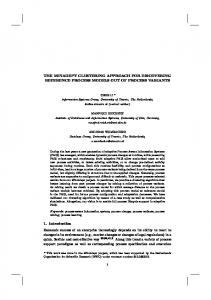
Another primary decision that the analyst has to make before clustering group among multivariate observation is choosing the appropriate clustering algorithm. In this paper, single linkage-clustering algorithm is being chosen among several hierarchical clustering algorithms because it is the best technique for identifying elongated clusters that will be the inliers [4]. This algorithm will form an initial partition of N clusters and then proceed to reduce the number of clusters one at a time until all N observations is in a single cluster. Single linkage mergers cluster based on the distance (“similarity measure”) between the two closest observations in each cluster and because of this, it

JTDIS45C[B]new.pmd

17

01/13/2009, 09:55

18

NURULHUDA FIRDAUS, HABSHAH, & NORANITA FAIRUS

11 20 30 34

3 5

1 10 25 28 2 4 45 43 12 40 42 46 13 33 38 6 44 18 41 31 16 26 23 47 36 24 37 39 8 32 17 19 29 35 27 21 15 22

0.0

9

14

0.5

7

1.0

1.5

2.0

is commonly referred to as the “nearest neighbor” algorithms. The results of this algorithm can be seen on a dendogram, or what is commonly referred to as a cluster tree. The vertical axis of a cluster tree, refer to Figure 1, represents the Euclidean distance at which successive clusters join each other.

Figure 1 An example of cluster tree (dendogram)

Specifically, the cluster tree must be partitioned or “cut” at a certain height in order to determine how many groups (if any) are in the data set. This number of groups depends upon where the tree is cut. In this paper, the Mojena’s cutting rule is being selected as a cutting procedure since it is simple to calculate and it has shown that using this simple rule provides excellent cluster solutions in the context of regression [4]. Mojena’s cutting rule resembles a one-sided confidence interval based – on the N-1 heights (joining distance) of the cluster tree, formally is, h + α Sh where h is the average of the heights for all N-1 clusters, and Sh is the unbiased standard deviation of the heights and is a specified constant. Mojena initially suggested that α should be specified in the range of 2.75–3.50 [7]. However, [8] in a more comprehensive study, conclude that the best overall performance of Mojena’s stopping rule occurs when the value of a is 1.25. As a summarization, the procedures of clustering approach for multiple outlier detection are as follows: (i)

JTDIS45C[B]new.pmd

Standardized the predicted and residual values using the estimator chosen. xij − xi Standardization is done for each of the variable by computing zij = where si xij is the j th observation on the i th variable.

18

01/13/2009, 09:55

THE PERFORMANCE OF CLUSTERING APPROACH WITH ROBUST MM-ESTIMATOR

19

(ii) Cluster the observation using single linkage clustering algorithm with pairs of standardized predicted and residuals values as the similarity measure in Euclidean distance. Obtain the cluster tree. (iii) Cut the tree and form groups at a height of h + α Sh based from the Mojena’s stopping rule. (iv) Identify the group with a majority of the observations in as the inliers observation and other observations out as outlying observations. 3.0 MM-ESTIMATOR AND BOOTSTRAP RESAMPLING A new improved estimator with higher efficiency for high breakdown estimates like Least Median Square (LMS) and Least Trimmed Square (LTS) were introduced by Yohai [9]. He called this new class of estimators as MM-Estimators. These estimates are defined in three stages, which are as follows: (i)

Take estimate T0,n of θ0 with high breakdown point, possibly 0.5.

(ii) Compute the residuals, ri(T0,n) = yi – T0,′ n xi ,1 ≤ i ≤ n and compute the M-scale

( ) ∑ ρ (u / s ) = b where b is defined by Eφ(ρ(u))

sn = s(r(T0,n)) defined by 1 n

n

i =1

i

= b and where φ stands for the standard normal distribution, use a constant b such that b/a = 0.5 where a = max ρ0(u). (iii) Let ρ1 be another function such that ρ1 (u ) ≤ ρ 0 (u ) sup ρ1(u) = sup ρ0(u) = a. Let ψ 1 = ρ1′ . Then the MM-estimate T1,n is defined as any solution of n

∑ψ 1 (ri (θ ) / sn ) xi = 0 which i =1

verifies

S(T 1,n )

≤

S(T 0,n )

where

n

S (θ ) = ∑ ρ1 (ri (θ ) / sn ) and ρ1(0/0) is defined as 0. i =1

In any statistical inference, it is normally concerned in procuring the standard errors of the parameter estimates and constructing confidence intervals of the parameter of a model. One of the methods that can be used to calculate confidence intervals is by using bootstrap method introduced by Efron [10]. This is a computer intensive based method that can substitute theoretical assumptions and analysis with considerable amount of computation. The advantage of using bootstrap method is that it does not require the normality assumption. This method makes use of re-sampling scheme where bootstrap samples are obtained. The bootstrap samples are repeated samples of the same size as the observed sample taken with replacement from the observed sample. The algorithm used in bootstrap re-sampling is as follows: (i)

∧

Fit a model to the original sample of observation to get β .

JTDIS45C[B]new.pmd

19

01/13/2009, 09:55

20

NURULHUDA FIRDAUS, HABSHAH, & NORANITA FAIRUS ∧

∧

(ii) Construct F , putting [(mass) × 1/n] at each observed residuals, F : [(mass) × 1/n] ∧

∧

at each ε i = yi – f(xi,β ), i = 1,2,…,n

∧

∧ ∧ ∧ (iii) Draw a bootstrap data set, *y i = f (xi,β ) + ε where ε are from F . ∧∗ (iv) Compute for the β bootstrap data set. (v) Repeat the number of bootstrap replication, B times for step 3 and 4, obtaining ∧∗1 ∧∗2

∧∗B

bootstrap replications β , β ,..., β . (vi) Estimate the bootstrap standard errors, by taking square root to the main diagonal of the covariance matrix, B

T

∧

COV =

∧ ∗.   ∧ ∗ b ∧ ∗.  ∧ ∗. 1 B  ∧b  β − β   β − β  where β = ∑ B − 1 b =1   

∧ ∗b

∑β b =1

B

(2)

The number of bootstrap replication, B depends on the applications where for standard errors estimates, Efron [10] suggested B to be between 25 and 200. However, Efron and Tibshirani [11] pointed out that B = 100 or 200 are not adequate for confidence interval construction whereas the B value should be larger or equal to 500 or 1000. In this paper, the Bias Corrected and Accelerated confidence interval (BCa) are employed in constructing the bootstrap confidence intervals. 4.0 EXPERIMENT AND RESULT FINDINGS In this section, it describes the evaluation approach to study the performance of proposed estimator in multiple outlier identification. This analysis is carried out in 3 ways, first to compare the proposed estimator with other classical estimator which is Least Square (LS) and other robust estimator that is Least Trimmed Square (LTS) through the analyses on a classical multiple outlier data sets found in the literature and simulated multiple outlier data sets. Secondly, all these estimators are further analysis by Root Mean Square Error (RMSE) value and finally, bootstrap method is adapted to estimates the confidence interval for the regression coefficient. This method is applied to evaluate which of these estimators produced “good” coverage probability, “good” equitailness and have the shortest average confidence length. The Bias Corrected and Accelerated (BCa) are employed in constructing the bootstrap confidence intervals. 4.1 The Performance of Studied Estimator with Clustering Approach in Classical Multiple Outlier Data Sets Researchers have used many data sets to illustrate the multiple outlier problems in linear regression. However, of these data sets, a few are repeatedly referred in the literature and are commonly used by authors to validate or investigate the performance of a proposed identification technique. These data sets are referred as “classic” data

JTDIS45C[B]new.pmd

20

01/13/2009, 09:55

THE PERFORMANCE OF CLUSTERING APPROACH WITH ROBUST MM-ESTIMATOR

21

sets [4]. In this paper, the classical multiple outlier data sets that are being referred are Hertzsprung data set, wood gravity data set and Coleman data set in order to investigate the performance of LS estimator, LTS estimator and the proposed estimator that is MM-Estimator. Table 1 represents the results of the estimators using clustering approach in classical data sets. Based on Table 1, it can be seen that the MM-Estimator successfully identified all the outliers for all the data sets compared to the LS estimator and LTS estimator in the sense that there are masking and no swamping. Table 1 Estimator performance using clustering approach in classical multiple outlier data set Outlying observation identified Data set

Outlying observation

LS

Hertzsprung

11, 20, 30, 34

7, 14, 11, 20, 30, 34

Wood gravity Coleman

4, 6, 8, 19 3, 18

LS

LTS

MM

7, 14, 11, 11, 20, 30, 20, 30, 34 34

2

2

0

7, 11, 4, 6, 8, 19 4, 6, 8, 19 4, 6, 8, 19

2

0

0

0

0

0

3, 18

LTS

Number of observation swamped (False alarm)

3, 18

MM

3, 18

4.2 The Performance of Studied Estimator with Clustering Approach in Simulated Multiple Outlier Data Sets The performance of MM-Estimator in clustering approach advocated in this paper has been shown to perform well in the classical data sets. However, for further investigation, a procedure on artificially generated regression data sets is performed. The simulated data sets are carried out based on the factors and levels of a regression condition as illustrated in Table 2. The factors and the corresponding levels were chosen so that the performance of the estimator being proposed could be tested in a wide variety of regression conditions for each outlier scenario. Serbert [4] refers an outlier scenario as a placement of the outlying observation relative to the inliers observations. In each scenario, the outliers were placed away from the inliers by a specified distance. These outlier distances were measured in standard deviations of the inliers observations (s = 1). Table 2 Factors and levels for the simulated data sets

JTDIS45C[B]new.pmd

Factor

Level

Number of regressor variables (k) Number of observation in data set (n) Percentage of outlying observation (%) Outlier distance

1, 2 20, 40 10, 20, 40 5s, 10s

21

01/13/2009, 09:55

22

NURULHUDA FIRDAUS, HABSHAH, & NORANITA FAIRUS

In this paper, two types of outlier scenario are considered, refer to Figure 2. The letters in the figure represent the outlying groups of observations. These scenarios are considered because there are situations in which multiple outliers are highly influential but typical least squares outlying measures and influence diagnostic fail to identify them. Specifically, these scenarios contain groups of high leverage outliers which are the most difficult to identify [4]. For each of the simulations, the values of the inliers or “clean” observations of a regressor variable were selected at random from a uniform distribution. The distribution of the random error for both clean and outlying observation was N~ (0, 1). The approaches in creating multiple outlier data sets are proposed by Serbert [4]. The approach was to randomly generate n regression observations. Of this n observation, nc “clean” observations were generated and represent the non-outlying observation. Also generated were no observations that were the outliers (nc + no = n). The nc clean observations were generated according to the model yi c = β 0 + β1xic + ε i , i = 1,…… , nc

(3)

where xic is U(0, 20) and εi is N(0, 1) with β0 = 1, β1 = 5. The no outlying observations were generated according to the model

(

(4) ) where εi is N(0, 1). The term ( x + x -shift ) allows the outliers to be placed at a specified

yio = β 0 + β1 xio + xshift + yshift + ε i , i = 1,…… , no io

location in the x-space where xio is the sample mean of the observations xic generated from U~ (0, 20). The y-shift term allows the outliers to be placed at a specified distance away from the inliers in the y-space. The term of x-shift and y-shift used are the outlier distances that are listed in Table 2. Both shifts used the same values. The procedure illustrated above is for the case of one regressor variable. However, the same methodologies are extended for the multiple regression (k > 1) data sets. Next, the clustering approaches with regression model fit by LS estimator are built. The same procedures are being repeated with different estimator that is LTS estimator Scenario 1

Scenario 2

y

y

A

AB

B 0

20

x

0

20

Figure 2 An outlier scenario

JTDIS45C[B]new.pmd

22

01/13/2009, 09:55

x

THE PERFORMANCE OF CLUSTERING APPROACH WITH ROBUST MM-ESTIMATOR

23

and MM-Estimator. These procedures are applied to 1000 random data sets created according to the specified regression condition. The results of this analysis are presented in Tables 3 and 4. Code developments were done using S-Plus version 2000. From Tables 3 and 4, they clearly show that the proposed estimator with clustering approach Table 3 Result with 1000 simulation run for outlier scenario 1

No. of regressor (k)

1

2

Size of observation N = 20 N = 40 No. of success No. of success

Outlier distance σ) (σ

Outlier percentage (%)

LS

LTS

MM

LS

LTS

MM

5 10 5 10 5 10

10 10 20 20 40 40

524 774 286 527 245 561

842 900 932 954 841 867

975 982 992 998 999 1000

642 784 415 696 467 601

897 914 957 974 906 925

986 989 997 999 1000 1000

5 10 5 10 5 10

10 10 20 20 40 40

741 823 912 948 761 800

944 967 973 983 921 947

964 976 987 994 999 1000

821 898 905 951 700 821

961 981 980 990 935 959

978 986 991 999 999 1000

Table 4 Result with 1000 simulation run for outlier scenario 2

No.of regressor (k)

1

2

JTDIS45C[B]new.pmd

Size of observation N = 20 N = 40 No. of success No. of success

Outlier distance σ) (σ

Outlier percentage (%)

LS

LTS

MM

LS

LTS

MM

5 10 5 10 5 10

10 10 20 20 40 40

489 602 600 642 574 677

997 820 921 937 907 924

1000 1000 995 999 999 998

498 621 632 700 531 547

998 987 970 990 925 956

1000 999 998 998 999 1000

5 10 5 10 5 10

10 10 20 20 40 40

597 633 645 659 421 497

957 989 900 964 804 912

997 1000 1000 1000 998 1000

601 640 655 701 501 513

994 997 935 977 937 951

1000 1000 999 997 1000 999

23

01/13/2009, 09:55

24

NURULHUDA FIRDAUS, HABSHAH, & NORANITA FAIRUS

is the best identification method in multiple outlier detection. The properties of this proposed estimator with a high breakdown point and high efficiency together with clustering procedure make the identification of multiple outliers in the simulated data set easy. 4.3

The Performance of Studied Estimator with Clustering Approach in Terms of Root Mean Square Error (RMSE) Value

The performance of these estimator in clustering approach were investigated further in terms of value of Root Mean Square Error (RMSE) in two situations namely “cleaned” data sets and “with outlier” data sets. The data were generated according to the sampling scheme that has been discussed in Section 4.2. For each simulation, sample of size 25 and 50 are being considered for a set of “clean” data and a set of data with outliers. In each simulation run, there were 1000 replications with some summary compute such 1 m ∧ as the mean estimated values, β j = ∑ β (j k ) which yield the bias β j − β j . The m k =1 mean squared error (MSE) is given by ∧

( ) (

MSE β j = β − β j

)

2

m

(

∧

(k ) + 1m ∑ β j − β j

k =1

∧

( )

)

2

12

(5)

Therefore, the root means squared error is given by  MSE β j  . This computation is done using S-Plus version 2000. Tables 5 and 6 exhibit the result of mean estimated values and Root Mean Squared Error (RMSE) for the estimators being studied. The values in the parenthesis are for sample of size 50. From the analysis, in the normal situation that is “clean” data sets, the mean estimated values and the RMSE of the MM-Estimator, LTS and LS are reasonably close to each other. However, the LS performance deteriorates badly when there are outliers in the data set. This can be seen from the high values of RMSE for the LS estimates. The robust estimator seems to perform reasonably better than the LTS and the classical estimator by referring to the values of the RMSE, which constantly shows that the value of the root mean square error (RMSE) of the LTS and MM estimator are always smaller than LS estimator. However, it can be noted that the MM columns have smaller value of root mean square error (RMSE) compared to the LTS in the presence of 40% of outliers. This shows that, although the LTS estimator is robust to the presence of the outlier, but yet its breakdown point will be affected by the presence of large cloud of outliers. Therefore, these indicate that the LTS estimator has slightly lower breakdown point and efficiency compared to the MM estimator that has high breakdown point and high efficiency in the presence of large number of outliers. Moreover, the accuracy of the estimates seem to increase as the sample sizes

JTDIS45C[B]new.pmd

24

01/13/2009, 09:55

JTDIS45C[B]new.pmd

25

0.0214 (0.0052)

β1

01/13/2009, 09:55

0.0214 (0.0052)

β1

5.0000 (5.0000)

β1

0.0215 (0.0075)

1.0024 (1.0053)

β0

β0

LS

Parameter

RMSE

0.00203 (0.00852)

0.0092 (0.01243)

5.0000 (5.0000)

1.0089 (1.0090)

Normal LTS

0.00181 (0.00341)

0.00418 (0.00831)

5.0000 (5.0000)

1.000 (1.0001)

MM

0.4470 (0.5621)

9.1376 (11.1711)

4.5620 (4.4858)

10.1372 (12.1688)

LS

0.00310 (0.0225)

0.02292 (0.0249)

5.00195 (5.00054)

0.97720 (0.98926)

0.00131 (0.01756)

0.00948 (0.01584)

5.0001 (5.0021)

1.0001 (1.0012)

10% outliers LTS MM

2.12779 (2.17278)

14.2419 (20.5096)

2.8892 (2.95698)

1.24274 (0.9323)

0.9732 (1.1605)

3.9900 (4.3943)

29.7841 (24.5947)

0.00926 (0.00094)

0.00684 (0.00325)

4.7801 (4.1214)

25.12503 (18.76102)

40% outliers LTS MM

46.2411 (45.5035)

LS

0.00203 (0.00852)

0.0092 (0.01243)

5.0000 (5.0000)

1.0089 (1.0090)

Normal LTS

.00181 (0.00341)

0.00418 (0.0831)

5.0000 (5.0000)

1.000 (1.0001)

MM

0.7339 (0.7244)

8.7367 (10.2933)

4.3555 (4.4870)

9.7296 (7.2725)

LS

0.03407 (0.0437)

0.0342 (0.0471)

5.0006 (5.0012)

0.99684 (0.9824)

0.00959 (0.00981)

0.0175 (0.0284)

5.0023 (5.0001)

1.0761 (1.0041)

10% outliers LTS MM

2.0452 (2.1046)

14.5803 (20.7672)

2.9562 (2.9168)

21.5801 (21.7651)

LS

0.4361 (0.2230)

0.2963 (1.2966)

5.3008 (5.1675)

1.9455 (0.6230)

0.00987 (0.005495)

0.0476 (0.02876)

5.1420 (5.1041)

1.8796 (1.5614)

40% outliers LTS MM

Table 6 Result of Root Mean Square Error (RMSE) value based on outlier scenario 2 for N = 25 and N = 50a and p = 2

0.0215 (0.0075)

5.0000 (5.0000)

β1

β0

1.0024 (1.0053)

β0

RMSE

LS

Parameter

Table 5 Result of Root Mean Square Error (RMSE) value based on outlier scenario 1 for N = 25 and N = 50a and p = 2 THE PERFORMANCE OF CLUSTERING APPROACH WITH ROBUST MM-ESTIMATOR 25

26

NURULHUDA FIRDAUS, HABSHAH, & NORANITA FAIRUS

increased from N = 25 to N = 50 for both situations, either in a “clean” data sets or contaminated data sets. 4.4 The Performance of Studied Estimator with Clustering Approach in Terms of Coverage Probabilities for Bias Corrected and Accelerated (BCa) Confidence Interval A series of simulation was conducted, one on a simulated data without outliers and another on a simulated data set with 10% and 20% outliers. Again the same simulation procedures are being considered as described earlier in Section 4.2. About 1000 bootstrap samples were drawn from a sample size of 20 and 40 and a bootstrap 95% confidence interval was constructed using Bias Corrected and Accelerated (BCa) method. This method was chosen since it has shown that Bias Corrected and Accelerated (BCa) confidence interval possesses a “good” coverage probability, “good” equitailness and narrowest average interval length [12]. In this series of simulation, 100 replications were executed to determine the percentage of times the true value of the parameter estimates was contained in the interval, and then the average length was calculated. The same procedure is repeated for the data with 10% and 20% outliers. It is important to note here that the procedures were repeated for both samples of size N = 20 and N = 40 in “clean” data sets and contaminated data sets. The results of the simulation studies are shown in Table 7. We would expect that a more robust method would be the one with “good” coverage probability, “good” equitailness and have the shortest average confidence length. From Table 7 it can be observed that for N = 20 and N = 40 with the “clean” data sets, the confidence intervals for the LS, LTS and MM are reasonably closed to the nominal value of 0.95. Nevertheless, the average lengths for the LS and LTS are longer than the MM confidence intervals. On the other hand, the confidence intervals for the LS give the worst results in the presence of outliers in the data set. Its coverage probability was very small and they displayed very bad equitailness, besides, its average confidence lengths are longer compared to the other estimators. However, the MMEstimator’s coverage probability is in best agreement with the 95% and its lower and upper coverage are reasonably closed. Although the LTS confidence intervals estimates are quite good both in terms of coverage probability and average length compared to LS confidence interval, but it cannot outperformed the MM estimator. This can be seen by looking at the coverage probabilities for MM confidence intervals that are constantly high and closer to 95%, followed by the LTS and LS confidence intervals. Its average length is also the shortest compared to the other two confidence intervals. Thus, it can be concluded that the MM-Estimator confidence intervals have all the criteria’s to be the best estimator since they have ‘good’ coverage probability, ‘good’ equitailness and the shortest average confidence length.

JTDIS45C[B]new.pmd

26

01/13/2009, 09:55

THE PERFORMANCE OF CLUSTERING APPROACH WITH ROBUST MM-ESTIMATOR

Table 7

Coverage probabilities and average width for the LS, LTS and MM-Estimator at N = 20, k=2

No outlier

Method

Coverage

Lower coverage

Upper coverage

Average width

LS

94 (93) 96 (95) 98 (97)

2 (3) 1 (2) 0 (1)

4 (4) 3 (3) 2 (2)

1.467 (1.132) 0.085 (0.085) 0.043 (0.013)

92 (91) 96 (94) 97 (96)

3 (4) 1 (3) 1 (1)

5 (5) 3 (3) 2 (3)

1.562 (1.562) 0.091 (0.093) 0.032 (0.032)

88 (75) 92 (85) 94 (94)

8 (17) 3 (6) 2 (3)

4 (8) 5 (9) 4 (3)

1.672 (2.692) 1.124 (1.028) 0.241 (0.187)

82 (70) 90 (87) 95 (95)

12 (18) 3 (3) 2 (2)

6 (12) 7 (10) 5 (5)

1.954 (3.054) 1.103 (1.380) 1.095 (1.085)

45 (4) 89 (83) 92 (95)

40 (86) 4 (7) 3 (0)

15 (10) 7 (10) 5 (5)

2.856 (19.585) 1.324 (1.455) 0.024 (0.074)

58 (28) 75 (85) 90 (96)

32 (42) 14 (7) 3 (1)

10 (30) 11 (8) 7 (3)

3.957 (9.757) 1.741 (2.958) 0.086 (0.029)

∧

β0

LTS MM LS

∧

β1

LTS MM

10% outlier LS ∧

β0

LTS MM LS

∧

β1

LTS MM

20% outlier LS ∧

β0

LTS MM LS

∧

β1

LTS MM

The figures for n = 50 are shown in parenthesis

JTDIS45C[B]new.pmd

27

27

01/13/2009, 09:55

28

NURULHUDA FIRDAUS, HABSHAH, & NORANITA FAIRUS

5.0 CONCLUSION This paper proposed a clustering method with robust estimator that is MM-Estimator for multiple outlier detection in linear regression. It has been revealed that the proposed method performed excellently on the classical multiple outliers data sets found in the literature and a wide variety of simulated multiple outlier data sets. Moreover, it has been clearly shown that the MM-Estimator in clustering approach performed reasonably well with any percentage of outliers, any number of regressor variables and any sample sizes followed by LTS and LS-based estimator. Since the MM-based estimator is found to be the best estimator and more easily in identifying the multiple outlying observations, thus the properties of MM-Estimator, LTS and LS estimator are investigated further in terms of the Root Mean Square Error (RMSE) value and Coverage Probabilities Of Bias Corrected and Accelerated (BCa) Confidence Interval. From the analysis, it has been shown that the MM-Estimator is more robust compared to the LTS and the LS estimator in the presence of multiple outlier in the data sets. ACKNOWLEDGEMENTS We wish to thank Associate Professor Dr. Habshah Midi from Institute for Mathematical Research (INSPEM), Universiti Putra Malaysia for her boundless and instructive help and criticism. Without her assistance and expert knowledge contribution in Robust Statistics and Bootstrap Re-sampling, this paper would not have been possible. REFERENCES [1] [2] [3] [4] [5] [6] [7] [8] [9] [10] [11] [12]

JTDIS45C[B]new.pmd

Barnett, V. and T. Lewis. 1994. Outliers in Statistical Data. 3rd edition. Great Britain: John Willey. Rousseeuw, P. J. and A. M. Leroy. 1987. Robust Regression and Outlier Detection. New York: John Willey & Sons. Hadi, A. S. and J. S. Simonoff. 1993. Procedure of the Identification of Multiple Outliers in Linear Model. Journal of the American Statistical Association. 88: 1264-1272. Serbert, D. M., D. C. Montgomery, and D. Rollier. 1998. A Clustering Algorithm for Identifying Multiple Outliers in Linear Regression. Computational Statistic and Data Analysis. 27: 461-484. Robiah, A., S. Halim, and M. Nor. 2000. Identifying Multiple Outliers in Linear Regression: Robust Fit and Clustering Approach, Congress of Science and Technology 2000, Malaysia. Everitt, B. S. 1993. Cluster Analysis. 3rd edition. New York: Halsted Press. Mojena, R. 1997. Hierarchical Grouping Methods and Stopping Rule: An Evaluation. The Computer Journal. 20: 359-363. Miligan, G. W. and M. C. Cooper. 1985. An Examination of Procedures for Determining the Number of Clusters in a Data Set. Psychometrika. 50(2): 159-179. Yohai, V. J. 1987. High Breakdown-Point and High Efficiency Robust Estimates for Regression. The Annals of Statistics. 15: 642-656. Efron, B. 1979. Bootstrap Methods: Another Look at the Jackknife. The Annals of Statistics. 7: 1-26. Efron, B. and R. J. Tibshirani. 1993. Introduction to the Bootstrap. New York: Chapman and Hall. Midi, H. 2000. Bootstrap Methods in a Class of Non Linear Regression Models. Pertanika Journal of Science & Technology. 8(2): 175-189.

28

01/13/2009, 09:55