The Quantum Schur Transform: I. Efficient Qudit Circuits

The Quantum Schur Transform: I. Efficient Qudit Circuits D. Bacon Dept. of Computer Science and Engineering, Univ. of Washington, Seattle, WA, USA Santa Fe Institute, Santa Fe, NM 87501 USA Institute for Quantum Information, California Institute of Technology, Pasadena, CA, USA and Dept. of Physics, California Institute of Technology, Pasadena, CA, USA

arXiv:quant-ph/0601001v1 30 Dec 2005

I. Chuang Center for Bits and Atoms, Massachusetts Institute of Technology, Cambridge, MA, USA Dept. of Electrical Engineering and Computer Science, Massachusetts Institute of Technology, Cambridge, MA, USA and Dept. of Physics, Massachusetts Institute of Technology, Cambridge, MA, USA

A. Harrow Center for Bits and Atoms, Massachusetts Institute of Technology, Cambridge, MA, USA Dept. of Physics, Massachusetts Institute of Technology, Cambridge, MA, USA and Dept. of Computer Science, Univ. of Bristol, Bristol, U.K. (Dated: February 1, 2008) We present an efficient family of quantum circuits for a fundamental primitive in quantum information theory, the Schur transform. The Schur transform on n d dimensional quantum systems is a transform between a standard computational basis to a labelling related to the representation theory of the symmetric and unitary groups. If we desire to implement the Schur transform to an accuracy of ǫ, then our circuit construction uses a number of gates which is polynomial in n, d and log(ǫ−1 ). The important insights we use to perform this construction are the selection of the appropriate subgroup adapted basis and the Wigner-Eckart theorem. Our efficient circuit construction renders numerous protocols in quantum information theory computationally tractable and is an important new efficient quantum circuit family which goes significantly beyond the standard paradigm of the quantum Fourier transform.

I.

INTRODUCTION

The last decade has seen the development and expansion of a robust theory of quantum information[1–6]. The basic goal of this new work has been the identification and quantification of different information resources in situations where the laws of quantum theory are applied to the physical carriers of information. Quantum information theory has made great progress in understanding the optimal rates of the manipulation and transmission of quantum information. Despite this success, however, much of the work in quantum information theory may not be of practical value. This is because most of the work in quantum information theory has focused on protocols which allow for unbounded quantum computational resources. Thus while the transforms in the quantum information protocols are well defined, whether these transforms can be implemented with quantum circuits whose size scales efficiently with the size of the quantum information problem is often left unaddressed. An analogous situation arises classically, for example, in the theory of classical error correcting codes. On the one hand, we would like the classical error correcting code to attain some characteristic efficiency for communicating over a noisy channel. On the other hand, we would also like to design codes whose encoding and decoding does not significantly lag our communication. In order to be of practical value a classical error correcting code must use computational resources which scale at a reasonable rate. While the goal of performing classical coding tasks in polynomial or even linear time has long been studied, quantum information theory results have typically ignored questions of efficiency. For example, random quantum coding results (such as [7–10]) require an exponential number of bits to describe, and like classical random coding techniques, do not yield efficient algorithms. There are a few important exceptions. Some quantum coding tasks, such as Schumacher compression[3, 11], are essentially equivalent to classical circuits, and as such can be performed efficiently on a quantum computer by carefully modifying an efficient classical algorithm to run reversibly and to deal properly with ancilla systems[12]. Another example, which illustrates some of the challenges involved, is Ref. [13]’s efficient implementation of entanglement concentration[5]. Quantum key distribution[14] not only runs efficiently, but can be implemented with entirely, or almost entirely, single-qubit operations and classical computation. Fault tolerant quantum computing[15] usually seeks to perform error correction with as few gates as possible, although with

2 teleportation-based techniques[16, 17] computational efficiency may not be quite as critical to the threshold rate. Finally, some randomized quantum code constructions have been given efficient constructions using classical derandomization techniques in [18]. In this paper we present an efficient family of quantum circuits for a transform used ubiquitously[19–30] in quantum information protocols, the Schur transform. Our efficient construction of the Schur transform adds to the above list a powerful new tool for finding algorithms that implement quantum communication tasks. The Schur transform is a unitary transform on n d-dimensional quantum systems (n qudits). The basis change corresponding to the Schur transform goes from a standard computational basis on the n qudits to a labelling related to the representation theory of the symmetric and unitary groups; much like the Fourier transform, it thus transforms from a local to a more global, collective basis, which captures symmetries of the system. In this article we show how to efficiently implement the Schur transform as a quantum circuit. The size of the circuit we construct is polynomial in the number of qudits, n, the dimension of the individual quantum systems, d, and the log of accuracy to which we implement the transform, log(ǫ−1 ). Our efficient quantum circuit for the Schur transform makes possible efficient quantum circuits for numerous quantum information tasks: optimal spectrum estimation[19, 20], universal entanglement concentration[22], universal compression with optimal overflow exponent[23, 24], encoding into decoherence-free subsystems[26–29], optimal hypothesis testing[25], and quantum and classical communication without shared reference frames[30]. The central role of the Schur transform in all of these protocols is due to the fact that the symmetries of independent and identically distributed quantum states are naturally treated by the representation theory of the symmetric and unitary groups. Thus in addition to making practical these quantum information protocols, the Schur transform is an interesting new unitary transformation with an interpretation relating to these symmetries. There are many difficulties in designing an efficient quantum circuit for the Schur transform which we overcome in this paper. The first difficulty is in efficiently representing the basis used in the Schur transform, the Schur basis. A second difficulty comes in the actual circuit construction. In particular we would like to construct the Schur transform from a series of Clebsch-Gordan transforms. However, it is not at all obvious how to efficiently implement these Clebsch-Gordan transforms, nor is obvious that such a cascade can perform the complete Schur transform. Our resolution to these problems begins by our selection of certain subgroup-adapted bases for the Schur basis. In particular we use the Gel’fand-Zetlin basis[31] and the Young-Yamanouchi basis (sometimes called Young’s orthogonal basis)[32]. We note that subgroup-adapted bases are also used in constructing efficient quantum circuits for Fourier transforms over nonabelian finite groups[33]. However, we should emphasize that the Schur transform is not a Fourier transform over a finite group, although connections between such transforms and the Schur transform exist, and are discussed in part II of this paper. By choosing the Gel’fand-Zetlin basis and the Young-Yamanouchi basis, we are able to show that the Schur transform can be constructed from a cascade of Clebsch-Gordan transforms. Further, the use of the Gel’fand-Zetlin basis, combined with the Wigner-Eckart theorem, allows us to efficiently implement the Clebsch-Gordan transform. In particular the Wigner-Eckart theorem allows us to recursively express the d dimensional Clebsch-Gordan transform in terms of the d − 1 dimensional Clebsch-Gordan transform and small, efficiently implementable, unitary transforms. This produces an efficient recursive construction of the Clebsch-Gordan transform. Without the recursive structure we exploit, a naive circuit construction would seem to require 2 nO(d ) gates. Our recursive exploitation of the Wigner-Eckart theorem allows us to implement the ClebschGordan transform to accuracy ǫ using poly(d, log n, log 1/ǫ) gates. The total size of our circuit construction for the Schur transform is n poly(d, log n, log 1/ǫ). The outline of the paper is as follows. In Section II we introduce the Schur transform, along with basic concepts from representation theory, and review the numerous applications of the Schur transform in quantum information theory. In Section III we introduce the basis labelling scheme used in the Schur transformation using the concept of a subgroup-adapted basis. Once we have a concrete Schur basis defined, we describe the Clebsch-Gordan transform and explain how to use it to give an efficient circuit for the Schur transform in Sec. IV. Finally, we complete the algorithm in Sec. V by constructing an efficient circuit for the ClebschGordan transform. II.

THE SCHUR TRANSFORM AND ITS APPLICATIONS

Consider a system of n d-dimensional quantum systems: n qudits. Fix a standard computational basis |ii, i = 1 . . . d for the state space of each qudit: Cd . A basis for the system (Cd )⊗n is then |i1 i ⊗ |i2 i ⊗ · · · ⊗ |in i = |i1 , i2 , . . . , in i where ik = 1 . . . d. The Schur transform is a unitary transform on the standard basis

3 |i1 , i2 , . . . , in i. After the Schur transform, the standard computational basis is relabeled as |λi|pi|qi (symbols which we later define). In this section we review the basic representation theory necessary to understand the Schur basis and also review the applications of this transformation to different protocols in quantum information theory. A.

Representation theory background

The Schur transform is related to the representations of two groups on (Cd )⊗n , a representation of the symmetric group and a representation of the unitary group. We first recall the basics of representation theory before introducing these representations. For a more detailed description of representation theory, the reader should consult [34] for general facts about group theory and representation theory or [35] for representations of Lie groups. See also [36] for a more introductory and informal approach to Lie groups and their representations. Representations: For a complex vector space V , define End(V ) to be set of linear maps from V to itself (endomorphisms). A representation of a group G is a vector space V together with a homomorphism from G to End(V ), i.e. a function R : G → End(V ) such that R(g1 )R(g2 ) = R(g1 g2 ). If R(g) is a unitary operator for all g, then we say R is a unitary representation. Furthermore, we say a representation (R, V ) is finite dimensional if V is a finite dimensional vector space. In this paper, we will always consider complex finite dimensional, unitary representations and use the generic term ‘representation’ to refer to complex, finite dimensional, unitary representations. Also, when clear from the context, we will denote a representation (R, V ) simply by the representation space V . The reason we consider only complex, finite dimensional, unitary representations is so that we can use them in quantum computing. If d = dim V , then a d-dimensional quantum system can hold a unit vector in a representation V . A group element g ∈ G corresponds to a unitary rotation R(g), which can in principle be performed by a quantum computer. Homomorphisms: For any two vector spaces V1 and V2 , define Hom(V1 , V2 ) to be the set of linear transformations from V1 to V2 . If G acts on V1 and V2 with representation matrices R1 and R2 respectively, then the canonical action of G on Hom(V1 , V2 ) is given by the map from M to R2 (g)M R1 (g)−1 for any M ∈ Hom(V1 , V2 ). For any representation (R, V ) define V G to be the space of G-invariant vectors of V : i.e. V G := {|vi ∈ V : R(g)|vi = |vi ∀g ∈ G}. Of particular interest is the space Hom(V1 , V2 )G , which can be thought of as the linear maps from V1 to V2 which commute with the action of G. If Hom(V1 , V2 )G contains any invertible maps (or equivalently, any unitary maps) then we say that (R1 , V1 ) and (R2 , V2 ) are equivalent representations and write G

V1 ∼ = V2 . This means that there exists a unitary change of basis U : V1 → V2 such that for any g ∈ G, U R1 (g)U † = R2 (g). Dual representations: Recall that the dual of a vector space V is the set of linear maps from V to C and is denoted V ∗ . Usually if vectors in V are denoted by kets (e.g. |vi) then vectors in V ∗ are denoted by bras (e.g. hv|). If we fix a basis {|v1 i, |v2 i, . . .} for V then the transpose is a linear map from V to V ∗ given by |vi i → hvi |. Now, for a representation (R, V ) we can define the dual representation (R∗ , V ∗ ) by R∗ (g)hv ∗ | := hv ∗ |R(g −1 ). If we think of R∗ as a representation on V (using the transpose map to relate V and V ∗ ), then it is given by R∗ (g) = (R(g −1 ))T . When R is a unitary representation, this is the same as the conjugate representation R(g)∗ , where here ∗ denotes the entrywise complex conjugate. One can readily verify G ∼ V ∗ ⊗ V2 . that the dual and conjugate representations are indeed representations and that Hom(V1 , V2 ) = 1 Irreducible representations: Generically the unitary operators of a representation may be specified (and manipulated on a quantum computer) in an arbitrary orthonormal basis. The added structure of being a representation, however, implies that there are particular bases which are more fundamental to expressing the action of the group. We say a representation (R, V ) is irreducible (and call it an irreducible representaiton, or irrep) if the only subspaces of V which are invariant under R are the empty subspace {0} and the entire space V . For finite groups, any finite-dimensional complex representation is reducible; meaning it is decomposable into a direct sum of irreps. For Lie groups, we need additional conditions, such as demanding that the representation R(g) be rational; i.e. its matrix elements are polynomial functions of the matrix elements gij and (det g)−1 . We say a representation of a Lie group is polynomial if its matrix elements are polynomial functions only of the gij .

4 Isotypic decomposition: Let Gˆ be a complete set of inequivalent irreps of G. Then for any reducible representation (R, V ) there is a basis under which the action of R(g) can be expressed as R(g) ∼ =

nλ MM

rλ (g) =

λ∈Gˆ j=1

M

λ∈Gˆ

rλ (g) ⊗ Inλ

(1)

where λ ∈ Gˆ labels an irrep (rλ , Vλ ) and nλ is the multiplicity of the irrep λ in the representation V . Here we use ∼ = to indicate that there exists a unitary change of basis relating the left-hand size to the right-hand side.1 Under this change of basis we obtain a similar decomposition of the representation space V (known as the isotypic decomposition): G

V ∼ =

M

λ∈Gˆ

Vλ ⊗ Cnλ .

(2)

Thus while generically we may be given a representation in some arbitrary basis, the structure of being a representation picks out a particular basis under which the action of the representation is not just block diagonal but also maximally block diagonal: a direct sum of irreps. Moreover, the multiplicity space Cnλ in Eq. (2) has the structure of Hom(Vλ , V )G . This means that for any representation (R, V ), Eq. (2) can be restated as G

V ∼ =

M

λ∈Gˆ

Vλ ⊗ Hom(Vλ , V )G .

(3)

Since G acts trivially on Hom(Vλ , V )G , Eq. (1) remains the same. As with the other results in this chapter, a proof of Eq. (3) can be found in [35], or other standard texts on representation theory. The value of Eq. (3) is that the unitary mapping from the right-hand side (RHS) to the left-hand side (LHS) has a simple explicit expression: it corresponds to the canonical map ϕ : A ⊗ Hom(A, B) → B given by ϕ(a ⊗ f ) = f (a). Of course, this doesn’t tell us how to describe Hom(Vλ , V )G , or how to specify an orthonormal basis for the space, but we will later find this form of the decomposition useful. B.

The Schur Transform

We now turn to the two representations relevant to the Schur transform. Recall that the symmetric group Sn of degree n, is the group of all permutations of n objects. Then we have the following natural representation of the symmetric group on the space (Cd )⊗n : P(s)|i1 i ⊗ |i2 i ⊗ · · · ⊗ |in i = |is−1 (1) i ⊗ |is−1 (2) i ⊗ · · · ⊗ |is−1 (n) i

(4)

where s ∈ Sn is a permutation and s(i) is the label describing the action of s on label i. For example, if we are considering S3 and the permutation we are considering is the transposition s = (12), then P(s)|i1 , i2 , i3 i = |i2 , i1 , i3 i. (P, (Cd )⊗n ) is the representation of the symmetric group which will be relevant to the Schur transform. Note that P obviously depends on n, but also has an implicit dependence on d. Now we turn to the representation of the unitary group. Let Ud denote the group of d×d unitary operators. Then there is a representation of Ud given by the n-fold product action as Q(U )|i1 i ⊗ |i2 i ⊗ · · · ⊗ |in i = U |i1 i ⊗ U |i2 i ⊗ · · · ⊗ U |in i

(5)

for any U ∈ Ud . More compactly, we could write that Q(U ) = U ⊗n . (Q, (Cd )⊗n ) is the representation of the unitary group which will be relevant to the Schur transform.

1

G

∼ when relating representation spaces. In Eq. (1) and other similar isomorphisms, we instead explicitly We only need to use = specify the dependence of both sides on g ∈ G.

5 Since both P(s) and Q(U ) meet our above criteria for reducibility, they can be decomposed into a direct sum of irreps as in Eq. (1), Sn M P(s) ∼ Inα ⊗ pα (s) = α

Ud

Q(U ) ∼ =

M β

Imβ ⊗ qβ (U )

(6)

where nα (mβ ) is the multiplicity of the αth (βth) irrep pα (s) (qβ (U )) in the representation P(s) (Q(U )). At this point there is not necessarily any relation between the two different unitary transforms implementing the isomorphisms in Eq. (6). However, further structure in this decomposition follows from the fact that P(s) commutes with Q(U ): P(s)Q(U ) = Q(U )P(s). This implies, via Schur’s Lemma, that the action of the irreps of P(s) must act on the multiplicity labels of the irreps Q(U ) and vice versa. Thus, the simultaneous action of P and Q on (Cd )⊗n decomposes as Ud ×Sn M M Imα,β ⊗ qβ (U ) ⊗ pα (s) (7) Q(U )P(s) ∼ = α

β

where mα,β can be thought of as the multiplicity of the irrep pα (s) ⊗ qβ (U ) of the group Ud × Sn . Not only do P and Q commute, but the algebras they generate (i.e. A := P(C[Sn ]) = Span{P(s) : s ∈ Sn } and B := Q(C[Ud ]) = Span{Q(U ) : U ∈ Ud }) centralize each other[35], meaning that B is the set of operators in End((Cd )⊗n ) commuting with A and vice versa, A is the set of operators in End((Cd )⊗n ) commuting with B. This means that the multiplicities mα,β are either zero or one, and that each α and β appears at most once. Thus Eq. (7) can be further simplified to Ud ×Sn M Q(U )P(s) ∼ qλ (U ) ⊗ pλ (s) (8) = λ

where λ runs over some unspecified set. Finally, Schur duality (or Schur-Weyl duality)[35, 37] provides a simple characterization of the range of λ in Eq. (8) and shows how the decompositions are related for different values of n and d. To define Schur duality, we will first need to specify the irreps of Sn and Ud . Pd Let Id,n = {λ = (λ1 , λ2 , . . . , λd )|λ1 ≥ λ2 ≥ · · · ≥ λd ≥ 0 and i=1 λi = n} denote partitions of n into ≤ d parts. We consider two partitions (λ1 , . . . , λd ) and (λ1 , . . . , λd , 0, . . . , 0) equivalent if they differ only by trailing zeroes; according to this principle, In := In,n contains all the partitions of n. Partitions label irreps of Sn and Ud as follows: if we let d vary, then Id,n labels irreps of Sn , and if we let n vary, then Id,n labels polynomial irreps of Ud . Call these (pλ , Pλ ) and (qdλ , Qdλ ) respectively, for λ ∈ Id,n . We need the superscript d because the same partition λ canP label different irreps for different Ud ; on the other hand the Sn -irrep Pλ is uniquely labeled by λ since n = i λi . For the case of n qudits, Schur duality states that there exists a basis (which we label |λi|qλ i|pλ iSch and call the Schur basis) which simultaneously decomposes the action of P(s) and Q(U ) into irreps: Q(U )|λi|qλ i|pλ iSch = |λi(qdλ (U )|qλ i)|pλ iSch P(s)|λi|qλ i|pλ iSch = |λi|qλ i(pλ (s)|pλ i)Sch

and that the common representation space (Cd )⊗n decomposes as Ud ×Sn M Qdλ ⊗ Pλ . (Cd )⊗n ∼ =

(9)

(10)

λ∈Id,n

The Schur basis can be expressed as superpositions over the standard computational basis states |i1 , i2 , . . . , in i as X λ,q ,pλ [USch ]i1 ,iλ2 ,...,i |i1 i2 . . . in i, (11) |λ, qλ , pλ iSch = n i1 ,i2 ,...,in

where USch is the unitary transformation implementing the isomorphism in Eq. (10). Thus, for any U ∈ Ud and any s ∈ Sn , X |λihλ| ⊗ qdλ (U ) ⊗ pλ (s). USch Q(U )P(s)U†Sch = (12) λ∈Id,n

6 If we now think of USch as a quantum circuit, it will map the Schur basis state |λ, qλ , pλ iSch to the computational basis state |λ, qλ , pλ i with λ, qλ , and pλ expressed as bit strings. The dimensions of the irreps pλ and qdλ vary with λ, so we will need to pad the |qλ , pλ i registers when they are expressed as bit strings. We will label the padded basis as |λi|qi|pi, explicitly dropping the λ dependence. Later in the paper we will show how to do this padding efficiently with only a logarithmic spatial overhead. We will refer to the transform from the computational basis |i1 , i2 , . . . , in i to the basis of three strings |λi|qi|pi as the Schur transform. The Schur transform is shown schematically in Fig. 1. Notice that just as the standard computational basis |ii is arbitrary up to a unitary transform, the bases for Qdλ and Pλ are also both arbitrary up to a unitary transform, though we will later choose particular bases for Qdλ and Pλ . Example of the Schur transform—Let d = 2. Then for n = 2 there are two valid partitions, λ1 = 2, λ2 = 0 and λ1 = λ2 = 1. Here the Schur transform corresponds to the change of basis from the standard basis to the singlet and triplet basis: |λ = (1, 1), qλ = 0, pλ = 0iSch = √12 (|01i − |10i), |λ = (2, 0), qλ = +1, pλ = 0iSch = |00i, |λ = (2, 0), qλ = 0, pλ = 0iSch = √12 (|01i + |10i), and |λ = (2, 0), qλ = −1, pλ = 0iSch = |11i. Abstractly, then, the Schur transform then corresponds to a transformation |00i |01i |10i |11i

z }|   0 √1 − √1 2 2   0  1 01 1    0 √2 √2 0 0 0

{ 0 0  0 1

(13)

|λ = (3, 0), qλ = +3/2, pλ = 0iSch = |000i 1 |λ = (3, 0), qλ = +1/2, pλ = 0iSch = √ (|001i + |010i + |100i) 3 1 |λ = (3, 0), qλ = −1/2, pλ = 0iSch = √ (|011i + |101i + |110i) 3 |λ = (3, 0), qλ = −3/2, pλ = 0iSch = |111i.

(14)

USch

|λ = (1, 1), qλ = 0, pλ = 0iSch |λ = (2, 0), qλ = +1, pλ = 0iSch = |λ = (2, 0), qλ = 0, pλ = 0iSch |λ = (2, 0), qλ = −1, pλ = 0iSch

It is easy to verify that the λ = (1, 1) subspace transforms as a one dimensional irrep of U2 and as the alternating sign irrep of S2 and that the λ = (2, 0) subspace transforms as a three dimensional irrep of U2 and as the trivial irrep of S2 . Notice that the labeling scheme for the standard computational basis uses 2 qubits while the labeling scheme for the Schur basis uses more qubits (one such labeling assigns one qubit to |λi, none to |pi and two qubits to |qi). Thus we see how padding will be necessary to directly implement the Schur transform. To see a more complicated example of the Schur basis, let d = 2 and n = 3. There are again two valid partitions, λ = (3, 0) and λ = (2, 1). The first of these partitions labels to the trivial irrep of S3 and a 4 dimensional irrep of U3 . The corresponding Schur basis vectors can be expressed as

The second of these partitions labels a two dimensional irrep of S3 and a two dimensional irrep of U2 . Its Schur basis states can be expressed as 1 |λ = (2, 1), qλ = +1/2, pλ = 0iSch = √ (|100i − |010i) 2 1 |λ = (2, 1), qλ = −1/2, pλ = 0iSch = √ (|101i − |011i) 2 r |010i + |100i 2 √ |001i − |λ = (2, 1), qλ = +1/2, pλ = 1iSch = 3 6 r |101i + |011i 2 √ |λ = (2, 1), qλ = −1/2, pλ = 1iSch = |110i − . 3 6

(15)

We can easily verify that Eqns. (14) and (15) indeed transform under U2 and S3 the way we expect; not so easy however is generalizing this basis to any n and d, let alone coming up with a natural circuit relating this basis to the computational basis. However, note that pλ determines whether the first two qubits are in a singlet or a triplet state. This gives a hint of a recursive structure that we will exploit in Sec. III to describe Schur bases for any choice of n and d, and in Sec. IV to construct an efficient recursive algorithm for the Schur transform.

7 |i1 i |i2 i

|λi

|i3 i USch

.. .

|qi

|in i

|pi

|0i FIG. 1: The Schur transform. Notice how the direct sum over λ in Eq. (10) becomes a tensor product between the |λi register and the |qi and |pi registers. Since the number of qubits needed for |qi and |pi vary with λ, we need slightly more spatial resources, which are here denoted by the ancilla input |0i.

C.

Constructing Qdλ and Pλ using Schur duality

So far we have said little about the form of Qdλ and Pλ , other than that they are indexed by partitions. It turns out that Schur duality gives a straightforward description of the irreps of Ud and Sn . We will not use this explicit description to construct the Schur transform, but it is still helpful for understanding the irreps Qdλ and Pλ . As with the rest of this section, proofs and further details can be found in [35]. We begin by expressing λ ∈ Id,n as a Young diagram in which there are up to d rows with λi boxes in row i. For example, to the partition (4, 3, 1, 1) we associate the diagram

.

(16)

Now we define a Young tableau T of shape λ to be a way of filling the n boxes of λ with the integers 1, . . . , n, using each number once and so that integers increase from left to right and from top to bottom. For example, one valid Young tableau with shape (4, 3, 1, 1) is 1 4 6 7 2 5 8 3 9 . For any Young tableau T , define Row(T ) to be set of permutations obtained by permuting the integers within each row of T ; similarly define Col(T ) to be the permutations that leave each integer in the same column of T . Now we define the Young symmetrizer Πλ:T to be an operator acting on (Cd )⊗n as follows:    X dim Pλ  X Πλ:T := P(r) . (17) sgn(c)P(c)  n! c∈Col(T )

r∈Row(T )

It can be shown that the Young symmetrizer Πλ:T is a projection operator whose support is a subspace isomorphic to Qdλ . In particular USch Πλ:T U†Sch = |λihλ|⊗|y(T )ihy(T )|⊗IQdλ for some unit vector |y(T )i ∈ Pλ . Moreover, these vectors |y(T )i form a basis known as Young’s natural basis, though the |y(T )i are not orthogonal, so we will usually not work with them in quantum circuits. Using Young symmetrizers, we can now explore some more general examples of Qdλ and Pλ . If λ = (n), then the only valid tableau is 1 2 ··· n . The corresponding Sn -irrep P(n) is trivial and the Ud -irrep is given by the action of Q on the totally symmetric subspace of (Cd )⊗n , i.e. {|vi : P(s)|vi = |vi∀s ∈ Sn }. On the other hand, if λ = (1n ), meaning (1, 1, . . . , 1)

8 (n times), then the only valid tableau is 1 2 .. . . n The Sn -irrep P(1n ) is still one-dimensional, but now corresponds to the sign irrep of Sn , mapping s to sgn(s). The Ud -irrep Qd(1n ) is equivalent to the totally antisymmetric subspace of (Cd )⊗n , i.e. {|vi : P(s)|vi = sgn(s)|vi∀s ∈ Sn }. Note that if d > n, then this subspace is zero-dimensional, corresponding to the restriction that irreps of Ud are indexed only by partitions with ≤ d rows. Other explicit examples of Ud and Sn irreps are presented from a particle physics perspective in [38]. We also give more examples in Sec. III B, when we introduce explicit bases for Qdλ and Pλ . D.

Applications of the Schur Transform

The Schur transform is useful in a surprisingly large number of quantum information protocols. Here we, review these applications, with particular attention to the use of the Schur transform circuit in each protocol. We emphasize again that our construction of the Schur transform simultaneously makes all of these tasks computationally efficient. 1.

Spectrum and state estimation

Suppose we are given many copies of an unknown mixed quantum state, ρ⊗n . An important task is to obtain an estimate for the spectrum of ρ from these n copies. An asymptotically good estimate (in the sense of large deviation rate) for the spectrum of ρ can be obtained by applying the Schur transform, measuring λ and taking the spectrum estimate to be (λ1 /n, . . . , λd /n)[19, 21]. Thus an efficient implementation of the Schur transform will efficiently implement the spectrum estimating protocol (note that it is efficient in d, not in log(d)). Estimating ρ reduces to measuring |λi and |qi, but optimal estimators have only been explicitly constructed for the case of d = 2[20]. Further, optimal quantum hypothesis testing can be obtained by a similar protocol[25]. 2.

Universal distortion-free entanglement concentration

Let |ψiAB be a bipartite partially entangled state shared between two parties, A and B. Suppose we are given many copies of |ψiAB and we want to transform these states into copies of a maximally entangled state using only local operations and classical communication. Further, suppose that we wish this protocol to work when neither A nor B know the state |ψiAB . Such a scheme is called a universal (meaning it works with unknown states |ψiAB ) entanglement concentration protocol, as opposed to the original entanglement concentration protocol described by Bennett et.al.[5]. Further we also would like the scheme to produce perfect maximally entangled states, i.e. to be distortion free. Universal distortion-free entanglement concentration can be performed[22] by both parties performing Schur transforms on their n halves of |ψiAB , measuring their |λi, discarding |qi and retaining |pi. The two parties will now share a maximally entangled state of varying dimension depending on what λ was measured. This dimension asymptotes to 2nH , where H is the entropy of one of the parties’ reduced mixed states. 3.

Universal Compression with Optimal Overflow Exponent

Measuring |λi weakly so as to cause little disturbance, together with appropriate relabeling, comprises a universal compression algorithm with optimal overflow exponent (rate of decrease of the probability that the algorithm will output a state that is much too large)[23, 24].

9 4.

Encoding and decoding into decoherence-free subsystems

Further applications of the Schur transform include encoding into decoherence-free subsystems[26–29]. Decoherence-free subsystems are subspaces of a system’s Hilbert space which are immune to decoherence due to a symmetry of the system-environment interaction. For the case where the environment couples identically to all systems, information can be protected from decoherence by encoding into the |pλ i basis. We can use the inverse Schur transform (which, as a circuit can be implemented by reversing the order of all gate elements and replacing them with their inverses) to perform this encoding: simply feed in the appropriate |λi with the state to be encoded into the |pi register and any state into the |qi register into the inverse Schur transform. Decoding can similarly be performed using the Schur transform. 5.

Communication without a shared reference frame

An application of the concepts of decoherence-free subsystems comes about when two parties wish to communicate (in either a classical or quantum manner) when the parties do not share a reference frame. The effect of not sharing a reference frame is the same as the effect of collective decoherence (the same random unitary rotation has been applied to each subsystem). Thus encoding information into the |pi register will allow this information to be communicated in spite of the fact that the two parties do not share a reference frame[30]. Just as with decoherence-free subsystems, this encoding and decoding can be done with the Schur transform. III.

SUBGROUP ADAPTED BASES AND THE SCHUR BASIS

In the last section, we defined the Schur transform in a way that left the basis almost completely arbitrary. To construct a quantum circuit for the Schur transform, we will need to explicitly specify the Schur basis. Since we want the Schur basis to be of the form |λ, q, pi, our task reduces to specifying orthonormal bases for Qdλ and Pλ . We will call these bases Qdλ and Pλ , respectively. We will choose Qdλ and Pλ to both be a type of basis known as a subgroup-adapted basis. In Sec. III A we describe the general theory of subgroup-adapted bases, and in Sec. III B, we will describe subgroupadapted bases for Qdλ and Pλ . As we will later see, the properties of these bases are intimately related to the structure of the algorithms that work with them. In this section, we will show how the bases can be stored on a quantum computer with a small amount of padding, and in the following sections we will show how the subgroup-adapted bases described here enable efficient implementations of Clebsch-Gordan and Schur duality transforms. A.

Subgroup Adapted Bases

Here we review the basic idea of a subgroup adapted basis. We assume that all groups we talk about are finite or compact Lie groups. Suppose (r, V ) is an irrep of a group G and H is a proper subgroup of G. We will construct a basis for V via the representations of H. Begin by restricting the input of r to H to obtain a representation of H, which we call (r|H , V↓H ). Note that unlike V , V↓H may be reducible. In fact, if we let (r′α , Vα′ ) denote the irreps of H, then V↓H will decompose under the action of H as H

V↓H ∼ =

M

ˆ α∈H

Cnα ⊗ Vα′

(18)

or equivalently, r|H decomposes as r(h) = r↓H (h) ∼ =

M

ˆ α∈H

Inα ⊗ r′α (h)

(19)

ˆ runs over a complete set of inequivalent irreps of H and nα is the branching multiplicity of the where H irrep labeled by α. Note that since r is a unitary representation, the subspaces corresponding to different

10 irreps of H are orthogonal. Thus, the problem of finding an orthonormal basis for V now reduces to the problem of (1) finding an orthonormal basis for each irrep of H, Vα′ and (2) finding orthonormal bases for the multiplicity spaces Cnα . The case when all the nα are either 0 or 1 is known as multiplicity-free branching. When this occurs, we only need to determine which irreps occur in the decomposition of V , and find bases for them. Now consider a group G along with a tower of subgroups G = G1 ⊃ G2 ⊃ · · · ⊃ Gk−1 ⊃ Gk = {e} where {e} is the trivial subgroup consisting of only the identity element. For each Gi , denote its irreps by Vαi , for α ∈ Gˆi . Any irrep Vα11 of G = G1 decomposes under restriction to G2 into G2 -irreps: say that Vα22 appears nα1 ,α2 times. We can then look at these irreps of G2 , consider their restriction to G3 and decompose them into different irreps of G3 . Carrying on in such a manner down this tower of subgroups will yield a labeling for subspaces corresponding to each of these restrictions. Moreover, if we choose orthonormal bases for the multiplicity spaces, this will induce an orthonormal basis for G. This basis is known as a subgroup-adapted basis and basis vectors have the form |α2 , m2 , α3 , m3 , . . . , αn , mn i, where |mi i is a basis vector for the (nαi−1 ,αi -dimensional) . multiplicity space of Vαii in Vαi−1 i−1 If the branching for each Gi+1 ⊂ Gi is multiplicity-free, then we say that the tower of subgroups is canonical. In this case, the subgroup adapted basis takes the particularly simple form of |α2 , . . . , αn i, where each αi ∈ Gˆi and αi+1 appears in the decomposition of Vαi↓Gi+1 . Often we include the original irrep label α = α1 as well: |α1 , α2 , . . . , αk i. This means that there exists a basis whose vectors are completely determined (up to an arbitrary choice of phase) by which irreps of G1 , . . . , Gk they transform according to. Notice that a basis for the irrep Vα does not consist of all possible irrep labels αi , but instead only those which can appear under the restriction which defines the basis. The simple recursive structure of subgroup adapted bases makes them well-suited to performing explicit computations. Thus, for example, subgroup adapted bases play a major role in efficient quantum circuits for the Fourier transform over many nonabelian groups[33]. B.

Explicit orthonormal bases for Qdλ and Pλ

In this section we describe canonical towers of subgroups for Ud and Sn , which give rise to subgroupadapted bases for the irreps Qdλ and Pλ . These bases go by many names: for Ud (and other Lie groups) the basis is called the Gel’fand-Zetlin basis (following [31]) and we denote it by Qdλ , while for Sn it is called the Young-Yamanouchi basis, or sometimes Young’s orthogonal basis (see [32] for a good review of its properties) and is denoted Pλ . The constructions and corresponding branching rules are quite simple, but for proofs we again refer the reader to [35]. The Gel’fand-Zetlin basis for Qdλ — For Ud , it turns out that the chain of subgroups {1} = U0 ⊂ U1 ⊂ . . . ⊂ Ud−1 ⊂ Ud is a canonical tower. For c < d, the subgroup Uc is embedded in Ud by Uc := {u ∈ Ud : u|ii = |ii for i = c + 1, . . . , d}. In other words, it corresponds to matrices of the form   u 0 , U ⊕ Id−c :=  (20) 0 Id−c where u is a c × c unitary matrix. Since the branching from Ud to Ud−1 is multiplicity-free, we obtain a subgroup-adapted basis Qdλ , which is known as the Gel’fand-Zetlin (GZ) basis. Our only free choice in a GZ basis is the initial choice of basis |1i, . . . , |di for Cd which determines the canonical tower of subgroups U1 ⊂ . . . ⊂ Ud . Once we have chosen this basis, specifying Qdλ reduces to knowing which irreps Qd−1 appear in the decomposition of Qdλ↓Ud−1 . µ Recall that the irreps of Ud are labeled by elements of Id,n with n arbitrary. This set can be denoted by d Zd++ := ∪n Id,n = {λ ∈ Zd : λ1 ≥ . . . ≥ λd ≥ 0}. For µ ∈ Zd−1 ++ , λ ∈ Z++ , we say that µ interlaces λ and write µ-λ whenever λ1 ≥ µ1 ≥ λ2 . . . ≥ λd−1 ≥ µd−1 ≥ λd . In terms of Young diagrams, this means that µ is a valid partition (i.e. a nonnegative, nonincreasing sequence) obtained from removing zero or one boxes from each column of λ. For example, if λ = (4, 3, 1, 1) (as in Eq. (16)), then µ-λ can be obtained by removing any subset of the marked boxes below, although if the box marked ∗ on the second line is removed, then the other marked box on that line must also be removed. ∗ × ×

× (21)

11 Thus a basis vector in Qdλ corresponds to a sequence of partitions q = (qd = λ, . . . , q1 ) such that q1 -q2 - . . . -qd and qj ∈ Zj++ for j = 1, . . . , d. Again using λ = (4, 3, 1, 1) as an example, and choosing d = 5 (any d ≥ 4 is possible), we might have the sequence % q5

% q4

% q3

% q2

(22) q1

Observe that it is possible in some steps not to remove any boxes, as long as qj has no more than j rows. In order to work with the Gel’fand-Zetlin basis vectors on a quantum computer, we will need an efficient method to write them down. Typically, we think of d as constant and express our resource use in terms of n. Then an element of Id,n can be expressed with d log(n + 1) bits, since it consists of d integers between 0 and
n. (This is a crude upper bound on |Id,n | = n+d−1 d−1 , but for constant d it is good enough for our purposes.) A Gel’fand-Zetlin basis vector then requires no more than d2 log(n + 1) bits, since it can be expressed as d partitions of integers no greater than n into ≤ d parts. Here, we assume that all partitions have arisen from a decomposition of (Cd )⊗n , so that no Young diagram has more than n boxes. Unless otherwise specified, our algorithms will use this encoding of the GZ basis vectors. It is also possible to express GZ basis vectors in a more visually appealing way by writing numbers in the boxes of a Young diagram. If q1 - . . . -qd is a chain of partitions, then we write the number j in each box contained in qj but not qj−1 (with q0 = (0)). For example, the sequence in Eq. (22) would be denoted 1 1 2 5 2 3 3 3 5 .

(23)

Equivalently, any method of filling a Young diagram with numbers from 1, . . . , d corresponds to a valid chain of irreps as long as the numbers are nondecreasing from left to right and are strictly increasing from top to bottom. The resulting diagram is known as a semi-standard Young tableau and gives another way d of hQencoding a GZ basis vector; i hQthis time i using n log d bits. (It turns out the actual dimension of Qλ is d 1≤i p′n−1 or pn−1 = p′n−1 and pn−2 > p′n−2 or pn−1 = p′n−1 , pn−2 = p′n−2 and pn−3 > p′n−3 , and so on. Thus fn : Pλ → [|Pλ |] can be easily verified to be n X X dim Pµ . (29) fn (p) = fn (p1 , . . . , pn ) := 1 + k=2 µ∈pk − µ 3, then the partition (3, 2, 1, 1) would also appear. We now seek to define the CG transform as a quantum circuit. We specialize to the case where one of the input irreps is the defining irrep, but allow the other irrep to be specified by a quantum input. The resulting CG transform is defined as: X λ,(1) (36) |λihλ| ⊗ UCG . UCG = λ∈Zd ++

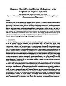
This takes as input a state of the form |λi|qi|ii, for λ ∈ Zd++ , |qi ∈ Qdλ and i ∈ [d]. The output is a superposition over vectors |λi|λ′ i|q ′ i, where λ′ = λ + ej ∈ Zd++ , j ∈ [d] and |q ′ i ∈ Qdλ′ . Equivalently, we could output |λi|ji|q ′ i or |ji|λ′ i|q ′ i, since (λ, λ′ ), (λ, j) and (λ′ , j) are all trivially related via reversible classical circuits. L To better understand the input space of UCG , we introduce the model representation Qd∗ := λ∈Zd Qdλ , ++ P with corresponding matrix qd∗ (U ) = λ |λihλ| ⊗ qdλ (U ). The model representation (also sometimes called the Schwinger representation) is infinite dimensional and contains each irrep once.2 Its basis vectors are of the form |λ, qi for λ ∈ Zd++ and |qi ∈ Qdλ . Since Qd∗ is infinite-dimensional, we cannot store it on a quantum computer and in this paper work only with representations Qdλ with |λ| ≤ n; nevertheless Qd∗ is a useful abstraction. Thus UCG decomposes Qd∗ ⊗ Qd(1) into irreps. There are two important things to notice about this version of the CG transform. First is that it operates simultaneously on different input irreps. Second is that different input irreps must remain orthogonal, so in order to to maintain unitarity UCG needs to keep the information of which irrep we started with. However, since λ′ = λ + ej , this information requires only storing some j ∈ [d]. Thus, UCG is a map from Qd∗ ⊗ Cd to Qd∗ ⊗ Cd , where the Cd in the input is the defining representation and the Cd in the output tracks which irrep we started with. |λi

|λi

|qi

UCG

|ii

|λ′ i

|qi

FIG. 2: Schematic of the Clebsch-Gordan transform. Equivalently, we could replace either the λ output or the λ′ output with j.

B.

Constructing the Schur Transform from Clebsch-Gordan Transforms

We now describe how to construct the Schur transform out of a series of Clebsch-Gordan transforms. Suppose we start with an input vector |i1 , . . . , in i ∈ (Cd )⊗n , corresponding to the Ud -representation (Qd(1) )⊗n . According to Schur duality (Eq. (10)), to perform the Schur transform it suffices to decompose (Qd(1) )⊗n into Ud -irreps. This is because Schur duality means that the multiplicity space of Qdλ must be isomorphic to Pλ . In other words, if we show that U

d (Qd(1) )⊗n ∼ =

M

λ∈Zd ++

Qdλ ⊗ Pλ′ ,

S

n then we must have Pλ′ ∼ = Pλ when λ ∈ Id,n and Pλ′ = {0} otherwise.

2

By contrast, L2 (Ud ), which will we not use, contains Qdλ with multiplicity dim Qdλ

(37)

15 To perform the Ud -irrep decomposition of Eq. (37), we simply combine each of |i1 i, . . . , |in i using the (1) = |(1)i, |i1 i and |i2 i into UCG which outputs CG one at a time. We start by inputting (1)transform, (2)  λ  λ and a superposition of different values of λ and |q2 i. Here λ(2) can be either (2, 0) or (1, 1) and  |q i ∈ Qdλ(2) . Continuing, we apply UCG to λ(2) |q2 i|i3 i, and output a superposition of vectors of the form 2(2)  (3)  λ λ |q3 i, with λ(3) ∈ Id,3 and |q3 i ∈ Qdλ(3) . Each time we are combining an arbitrary irrep λ(k) and an associated basis vector |qk i ∈ Qdλ(k) , together with a vector from the defining irrep |ik+1 i. This is repeated for k = 1, . . . , n − 1 and the resulting circuit is depicted in Fig. 3. j(1) i

j(1)i j i1 i

j i2 i

j i3 i j i4 i

UCG

j(2) i

UCG

j(3) i

UCG

b b b b

b b

b

j(n 2) i

b b b

b b

b b b

j in i

UCG

j(n 1) i j(n) i jqn i .

FIG. 3: Cascading Clebsch-Gordan transforms to produce the Schur transform. Not shown are any ancilla inputs to the Clebsch-Gordan transforms. The structure of inputs and outputs of the Clebsch-Gordan transforms are the same as in Fig. 2.

 Finally, we are left with a superposition of states of the form λ(1) , . . . , λ(n) |qn i, where |qn i ∈ Qdλ(n) , λ(k) ∈ Id,k and each λ(k) is obtained by adding a single box to λ(k−1) ; i.e. λ(k) = λ(k−1) + ejk for some ′ jk ∈ [d]. If we define λ = λ(n) and |qi  = |qn i, then we have the decomposition of Eq. (37) with Pλ (1) (n−1) spanned by the vectors λ , . . . , λ satisfying the constraints described above. But this is precisely the Young-Yamanouchi basis Pλ that we have defined in Sec. III! Since the first k qudits transform under Ud according to Qdλ(k) , Schur duality implies that they also transform under Sk according to Pλ(k) . Thus  we set |pi = λ(1) , . . . , λ(n−1) (optionally compressing to ⌈log |Pλ |⌉ qubits using the techniques described in the last section) and obtain the desired |λi|qi|pi. As a check on this result, note that each λ(k) is invariant under Q(Ud ) since U ⊗n acts on the first k qubits simply as U ⊗k .  If we choose not to perform the poly(n) steps to optimally compress λ(1) , . . . , λ(n−1) , we could instead have our circuit output the equivalent |j1 , . . . , jn−1 i, which requires only n log d qubits and asymptotically no extra running time. We can now appreciate the similarity between the Ud CG “add a box” prescription and the Sn−1 ⊂ Sn branching rule of “remove a box.” Schur duality implies that the representations Qdλ′ that are obtained by decomposing Qdλ ⊗ Qd(1) are the same as the Sn -irreps Pλ′ that include Pλ when restricted to Sn−1 . Define TCG (n, d, ǫ) to be the time complexity (in terms of number of gates) of performing a single Ud CG transform to accuracy ǫ on Young diagrams with ≤ n boxes. Then the total complexity for the Schur transform is n · (TCG (n, d, ǫ/n) + O(1)), possibly plus a poly(n) factor for compressing the Pλ register to ⌈log dim Pλ ⌉ qubits (as is required for applications such as data compression and entanglement concentration, cf. Sec. II D). In the next section we will show that TCG (n, d, ǫ) is poly(log n, d, log 1/ǫ), but first we give a step-by-step description of the algorithm for the Schur transform. Algorithm: Schur transform (plus optional compression) Inputs: (1) Classical registers d and n. (2) An n qudit quantum register |i1 , . . . , in i. Outputs: Quantum registers |λi|qi|pi, with λ ∈ Id,n , q ∈ Qdλ and p ∈ Pλ . Runtime: n · (TCG (n, d, ǫ/n) + O(1)) to achieve accuracy ǫ. (Optionally plus poly(n) to compress the Pλ register to ⌈log dim Pλ ⌉ qubits.)

16 Procedure:  1. Initialize λ(1) := |(1)i and |q1 i = |i1 i. 2. For k = 1, . . . , n − 1:   3. Apply UCG to λ(k) |qk i|ik+1 i to obtain output |jk i λ(k+1) |qk+1 i, where λ(k+1) = λ(k) + ejk . 4. Output |λi := λ(n) , |qi := |qn i and |pi := |j1 , . . . , jn−1 i. 5. (Optionally use Eq. (29) to reversibly map |j1 , . . . , jn−1 i to an integer p ∈ [dim Pλ ].)

This algorithm will be made efficient in the next section, where we efficiently construct the CG transform for Ud , proving that TCG (n, d, ǫ) = poly(log n, d, log 1/ǫ). V.

EFFICIENT CIRCUITS FOR THE CLEBSCH-GORDAN TRANSFORM

We now turn to the actual construction of the circuit for the Clebsch-Gordan transform described in Sec. IV A. To get a feel for the what will be necessary, we start by giving a circuit for the CG transform that 2 is efficient when d is constant; i.e. it has complexity nO(d ) , which is poly(n) for any constant value of d. 2 First recall that dim Qdλ ≤ (n + 1)d . Thus, controlled on λ, we want to construct a unitary transform on a D-dimensional system for D = maxλ∈Id,n dim Qdλ = poly(n). There are classical algorithms[39] to compute matrix elements of UCG to an accuracy ǫ1 in time poly(D) poly log(1/ǫ1 ). Once we have calculated all the relevant matrix elements (of which there are only polynomially many), we can (again in time poly(D) poly log(1/ǫ)) decompose UCG into D2 poly log(D) elementary one and two-qubit operations[40–43]. These can in turn be approximated to accuracy ǫ2 by products of unitary operators from a fixed finite set (such as Clifford operators and a π/8 rotation) with a further overhead of poly log(1/ǫ2 )[44, 45]. We can either assume the relevant classical computations (such as decomposing the D × D matrix into elementary gates) are performed coherently on a quantum computer, or as part of a polynomial-time classical Turing machine which outputs the quantum circuit. In any case, the total complexity is poly(n, log 1/ǫ) if the desired final accuracy is ǫ and d is held constant. The goal of this section is to reduce this running time to poly(n, d, log(1/ǫ)); in fact, we will achieve circuits of size poly(d, log n, log(1/ǫ)). To do so, we will reduce the Ud CG transform to two components; first, a Ud−1 CG transform, and second, a d × d unitary matrix whose entries can be computed classically in poly(d, log n, 1/ǫ) steps. After computing all d2 entries, the second component can then be implemented with poly(d, log 1/ǫ) gates according to the above arguments. This reduction from the Ud CG transform to the Ud−1 CG transform is a special case of the WignerEckart Theorem, which we review in Sec. V A. Then, following [39, 46], we use the Wigner-Eckart Theorem to give an efficient recursive construction for UCG in Sec. V B. Putting everything together, we obtain a quantum circuit for the Schur transform that is accurate to within ǫ and runs in time n·poly(log n, d, log 1/ǫ), optionally plus an additional poly(n) time to compress the |pi register. A.

The Wigner-Eckart Theorem and Clebsch-Gordan transform

In this section, we introduce the concept of an irreducible tensor operator, which we use to state and prove the Wigner-Eckart Theorem. Here we will find that the CG transform is a key part of the Wigner-Eckart Theorem, while in the next section we will turn this around and use the Wigner-Eckart Theorem to give a recursive decomposition of the CG transform. Suppose (r1 , V1 ) and (r2 , V2 ) are representations of Ud . Recall that Hom(V1 , V2 ) is a representation of Ud under the map T → r2 (U )T r1 (U )−1 for T ∈ Hom(V1 , V2 ). If T = {T1 , T2 , . . .} ⊂ Hom(V1 , V2 ) is a basis for a Ud -invariant subspace of Hom(V1 , V2 ), then we call T a tensor operator. Note that a tensor operator T is a collection of operators {Ti } indexed by i, just as a tensor (or vector) is a collection of scalars labeled by some index. For example, the Pauli matrices {σx , σy , σz } ⊂ Hom(C2 , C2 ) comprise a tensor operator, since conjugation by U2 preserves the subspace that they span. Since Hom(V1 , V2 ) is a representation of Ud , it can be decomposed into irreps. If T is a basis for one of these irreps, then we call it an irreducible tensor operator. For example, the Pauli matrices mentioned above comprise an irreducible tensor operator, corresponding to the three-dimensional irrep Q2(2) . Formally, we say that T ν = {Tqνν }qν ∈Qdν ⊂ Hom(V1 , V2 ) is an irreducible tensor operator (corresponding to the irrep Qdν ) if for

17 all U ∈ Ud we have r2 (U )Tqνν r1 (U )−1 =

X

qν′ ∈Qd ν

hqν′ |qdν (U )|qν iTqνν′ .

(38)

Now assume that V1 and V2 are irreducible (say V1 = Qdµ and V2 = Qdλ ), since if they are not, we could always decompose Hom(V1 , V2 ) into a direct sum of homomorphisms from an irrep in V1 to an irrep in V2 . We can decompose Hom(Qdµ , Qdλ ) into irreps using Eq. (3) and the identity Hom(A, B) ∼ = A∗ ⊗ B as follows: U

d Hom(Qdµ , Qdλ ) ∼ =

Ud

∼ =

M

Qdν ⊗ Hom(Qdν , Hom(Qdµ , Qdλ ))Ud

M

Qdν ⊗ Hom(Qdν , (Qdµ )∗ ⊗ Qdλ )Ud

M

Qdν ⊗ (Qdµ )∗ ⊗ (Qdν )∗ ⊗ Qdλ

M

Qdν ⊗ Hom(Qdµ ⊗ Qdν , Qdλ )Ud

ν∈Zd ++

ν∈Zd ++ Ud

∼ =

ν∈Zd ++ Ud

∼ =

ν∈Zd ++


Ud

(39)

Now consider a particular irreducible tensor operator Tν ⊂ Hom(Qdµ , Qdλ ) with components Tqνν where qν ranges over Qdν . We can define a linear operator Tˆ : Qdµ ⊗ Qdν → Qdλ by letting Tˆ|qµ i|qν i := Tqνν |qµ i

(40)

for all qµ ∈ Qdµ , qν ∈ Qdν and extending it to the rest of Qdµ ⊗ Qdν by linearity. By construction, Tˆ ∈ Hom(Qdµ ⊗ Qdν , Qdλ ), but we claim that in addition Tˆ is invariant under the action of Ud ; i.e. that it lies in Hom(Qdµ ⊗ Qdν , Qdλ )Ud . To see this, apply Eqns. (38) and (40) to show that for any U ∈ Ud , qµ ∈ Qdµ and qν ∈ Qdν , we have X   qdλ (U )Tˆ qdµ (U )−1 ⊗ qdν (U )−1 |qµ i|qν i = hqν′ |qdν (U )−1 |qν iqdλ (U )Tqνν′ qdµ (U )−1 |qµ i qν′ ∈Qd ν

=

X

qν′ ,qν′′ ∈Qd ν

hqν′′ |qdν (U )|qν′ ihqν′ |qdν (U )−1 |qν iTqνν′′ |qµ i

(41)

= Tqνν |qµ i = Tˆ|qµ i|qν i. λ Now, fix an orthonormal basis for Hom(Qdµ ⊗ Qdν , Qdλ )Ud and call it Mµ,ν . Then we can expand Tˆ in this basis as X Tˆα · α, (42) Tˆ = λ α∈Mµ,ν

where the Tˆα are scalars. Thus hqλ |Tqνν |qµ i =

X

λ α∈Mµ,ν

Tˆα hqλ |α|qµ , qν i.

(43)

This last expression hqλ |α|qµ , qν i bears a striking resemblance to the CG transform. Indeed, note that the multiplicity space Hom(Qdλ , Qdµ ⊗Qdν )Ud from Eq. (30) is the dual of Hom(Qdµ ⊗Qdν , Qdλ )Ud (which contains α), meaning that we can map between the two by taking the transpose. In fact, taking the conjugate transpose of Eq. (32) gives hqλ |α = qλ , α† Uµ,ν CG . Thus

hqλ |α|qµ , qν i = qλ , α† Uµ,ν (44) CG |qµ , qν i. The arguments in the last few paragraphs constitute a proof of the Wigner-Eckart theorem[47], which is stated as follows:

18 Theorem 1 (Wigner-Eckart) For any irreducible tensor operator Tν = {Tqνν }qν ∈Qdν ⊂ Hom(Qdµ , Qdλ ), λ there exist Tˆα ∈ C for each α ∈ Mµ,ν such that for all |qµ i ∈ Qdµ , |qν i ∈ Qdν and |qλ i ∈ Qdλ : hqλ |Tqνν |qµ i =

X

λ α∈Mµ,ν



Tˆα qλ , α† Uµ,ν CG |qµ , qν i.

(45)

Thus, the action of tensor operators can be related to a component Tˆα that is invariant under Ud and a component that is equivalent to the CG transform. We will use this in the next section to derive an efficient quantum circuit for the CG transform. B.

A recursive construction of the Clebsch-Gordan transform [d]

In this section we show how the Ud CG transform (which here we call UCG ) can be efficiently reduced to [d−1] [d] the Ud−1 CG transform (which we call UCG ). Our strategy, following [46], will be to express UCG in terms [d−1] of Ud−1 tensor operators and then use the Wigner-Eckart Theorem to express it in terms of UCG . After we [d] [d−1] have explained this as a relation among operators, we describe a quantum circuit for UCG that uses UCG as a subroutine. [d] First, we express UCG as a Ud tensor operator. For µ ∈ Zd++ , |qi ∈ Qdµ and i ∈ [d], we can expand [d]

UCG |µi|qi|ii as

[d]

UCG |µi|qi|ii = |µi

X

X

j∈[d] s.t. q′ ∈Qd µ+ej µ+ej ∈Zd ++

µ,j ′ Cq,i,q ′ |µ + ej i|q i.

(46)

µ,j µ,j for some coefficients Cq,i,q : Qdµ → Qdµ+ej by ′ ∈ C. Now define operators Ti

Tiµ,j =

X

q∈Qd µ

X

q′ ∈Qd µ+ej

µ,j ′ Cq,i,q ′ |q ihq|,

(47)

[d]

so that UCG decomposes as [d]

UCG |µi|qi|ii = |µi

X

j∈[d] s.t. µ+ej ∈Zd ++

|µ + ej iTiµ,j |qi.

(48)

[d]

Thus UCG can be understood in terms of the maps Tiµ,j , which are irreducible tensor operators in Hom(Qdµ , Qdµ+ej ) corresponding to the irrep Qd(1) . (This is unlike the notation of the last section in which the superscript denoted the irrep corresponding to the tensor operator.) The plan for the rest of the section is to decompose the Tiµ,j operators under the action of Ud−1 , so that we can apply the Wigner-Eckart theorem. This involves decomposing three different Ud irreps into Ud−1 irreps: the input space Qdµ , the output space Qdµ+ej and the space Qd(1) corresponding to the subscript i. [d]

Once we have done so, the Wigner-Eckart Theorem gives an expression for Tiµ,j (and hence for UCG ) in [d−1] terms of UCG and a small number of coefficients, known as reduced Wigner coefficients. These coefficients can be readily calculated, and in the next section we cite a formula from [46] for doing so. First, we examine the decomposition of Qd(1) , the Ud -irrep according to which the Tiµ,j transform. Recall Ud−1

µ,j d−1 is an that Qd(1) ∼ = Qd−1 (0) ⊕ Q(1) . In terms of the tensor operator we have defined, this means that Td

µ,j µ,j irreducible Ud−1 tensor operator corresponding to the trivial irrep Qd−1 (0) and {T1 , . . . , Td−1 } comprise an

irreducible Ud−1 tensor operator corresponding to the defining irrep Qd−1 (1) . Next, we would like to decompose Hom(Qdµ , Qdµ+ej ) into maps between irreps of Ud−1 . This is slightly more complicated, but can be derived from the Ud−1 ⊂ Ud branching rule introduced in Sec. III B. Recall that Ud−1 L Ud−1 L d−1 d−1 d ∼ Qdµ ∼ = µ′′ -µ+ej Qµ′′ . This is the moment that we anticipated µ′ -µ Qµ′ , and similarly Qµ+ej =

19 in Sec. III B when we chose our set of basis vectors Qdµ to respect these decompositions. As a result, a ′ vector |qi ∈ Qdµ can be expanded as q = (qd−1 , qd−2 , . . . , q1 ) = (µ′ , q(d−2) ) with qd−1 = µ′ ∈ Zd−1 ++ , µ -µ  d−1 d and q(d−2) = |qd−2 , . . . , q1 i ∈ Qµ′ . In other words, we will separate vectors in Qµ into a Ud−1 irrep label d−1 µ′ ∈ Zd−1 ++ and a basis vector from Qµ′ . This describes how to decompose the spaces Qdµ and Qdµ+ej . To extend this to decomposition of L L L Hom(Qdµ , Qdµ+ej ), we use the canonical isomorphism Hom( x Ax , y By ) ∼ = x,y Hom(Ax , By ), which holds for any sets of vector spaces {Ax } and {By }. Thus Ud−1

Hom(Qdµ , Qdµ+ej ) ∼ =

M

M

µ′ -µ

µ′′ -µ+ej

d−1 Hom(Qd−1 µ′ , Qµ′′ ).

(49a)

Sometimes we will find it convenient to denote the Qd−1 subspace of Qdµ by Qd−1 ⊂ Qdµ , so that Eq. (49a) µ′ µ′ becomes M Ud−1 M d Hom(Qd−1 ⊂ Qdµ , Qd−1 (49b) Hom(Qdµ , Qdµ+ej ) ∼ = µ′ µ′′ ⊂ Qµ+ej ). µ′ -µ

µ′′ -µ+ej

According to Eq. (49) (either version), we can decompose Tiµ,j as X X ′ ′′ |µ′′ ihµ′ | ⊗ Tiµ,j,µ ,µ . Tiµ,j = µ′ -µ

′

(50)

µ′′ -µ+ej

′′

Here Tiµ,j,µ ,µ ∈ Hom(Qd−1 ⊂ Qdµ , Qd−1 ⊂ Qdµ+ej ) and we have implicitly decomposed |qi ∈ Qdµ into µ′ µ′′  |µ′ i q(d−2) . The next step is to decompose the representions in Eq. (49) into irreducible components. In fact, we are d−1 d−1 d−1 not interested in the entire space Hom(Qd−1 µ′ , Qµ′′ ), but only the part that is equivalent to Q(1) or Q(0) , ′

′′

depending on whether i ∈ [d − 1] or i = d (since Tiµ,j,µ ,µ transforms according to Qd−1 (1) if i ∈ {1, . . . , d − 1} ′

′′

µ,j,µ ,µ and according to Qd−1 transforms under Ud−1 will give us (0) if i = d). This knowledge of how Ti ′

′′

two crucial simplifications: first, we can greatly reduce the range of µ′′ for which Tiµ,j,µ ,µ is nonzero, and ′ ′′ [d−1] second, we can apply the Wigner-Eckart theorem to describe Tiµ,j,µ ,µ in terms of UCG . d−1 The simplest case is Q(0) , when i = d: according to Schur’s Lemma the invariant component of d−1 ′ ′′ Hom(Qd−1 if µ′ = µ′′ . In µ′ , Qµ′′ ) is zero if µ 6= µ and consists of the matrices proportional to IQd−1 ′

other words

′ ′′ Tdµ,j,µ ,µ

′

′′

= 0 unless µ = µ , in which case

′ ′ Tdµ,j,µ ,µ

µ

′ ′ := Tˆ µ,j,µ ,0 IQd−1 for some scalar Tˆ µ,j,µ ,0 . µ′

(The final superscript 0 will later be convenient when we want a single notation to encompass both the i = d and the i ∈ {1, . . . , d − 1} cases.) µ,j,µ′ ,µ′′ The Qd−1 (1) case, which occurs when i ∈ {1, . . . , d − 1}, is more interesting. We will simplify the Ti operators (for i = 1, . . . , d − 1) in two stages: first using the branching rules from Sec. III B to reduce the number of nonzero terms and then by applying the Wigner-Eckart theorem to find an exact expression for them. Begin by recalling from Eq. (39) that the multiplicity of Qd−1 (1) in the isotypic decomposition of d−1 d−1 d−1 d−1 Ud−1 Hom(Qd−1 . According to the Ud−1 CG “add a box” µ′ , Qµ′′ ) is given by dim Hom(Qµ′ ⊗ Q(1) , Qµ′′ ) ′

′′

prescription (Eq. (33)), this is one if µ′ ∈ µ′′ −  and zero otherwise. Thus if i ∈ [d − 1], then Tiµ,j,µ ,µ is zero unless µ′′ = µ′ + ej ′ for some j ′ ∈ [d − 1]. Since we need not consider all possible µ′′ , we can define ′

′

µ,j,µ′ ,µ′ +e

j Tiµ,j,µ ,j := Ti . This notation can be readily extended to cover the case when i = d; define e0 = 0, ′ ′ ′ ′ so that the only nonzero operators for i = d are of the form Tdµ,j,µ ,0 := Tdµ,j,µ ,µ = Tˆ µ,j,µ ,0 IQd−1 . Thus, we ′

µ′

can replace Eq. (50) with

Tiµ,j =

X d−1 X

µ′ -µ j ′ =0

µ,j,µ′ ,µ′ +ej′

|µ′ + ej ′ ihµ′ | ⊗ Ti

.

(51) ′

′

Now we show how to apply the Wigner-Eckart theorem to the i ∈ [d − 1] case. The operators Tiµ,j,µ ,j d−1 map Qd−1 to Qd−1 µ′ µ′ +ej′ and comprise an irreducible Ud−1 tensor operator corresponding to the irrep Q(1) .

20 d−1 d−1 This means we can apply the Wigner-Eckart theorem and since the multiplicity of Qd−1 µ′ +ej′ in Qµ′ ⊗ Q(1) is one, the sum over′ the multiplicity label α has only a single term. The theorem implies the existence of a ′ set of scalars Tˆ µ,j,µ ,j such that for any |qi ∈ Qd−1 and |q ′ i ∈ Qd−1 , ′ ′ µ +ej′

µ

′

′

′ ′ [d−1] hq ′ |Tiµ,j,µ ,j |qi = Tˆ µ,j,µ ,j hµ′ , µ′ + ej ′ , q ′ |UCG |µ′ , q, ii. ′

′

(52) ′

′

Sometimes the matrix elements of UCG or Tiµ,j,µ ,j are called Wigner coefficients and the Tˆ µ,j,µ ,j are known as reduced Wigner coefficients. Let us now try to interpret these equations operationally. Eq. (48) reduces the Ud CG transform to a Ud tensor operator, Eq. (51) decomposes this tensor operator into d2 different Ud−1 tensor operators (weighted ′ ′ by the Tˆ µ,j,µ ,j coefficients) and Eq. (52) turns this into a Ud−1 CG transform followed by a d × d unitary ′ ′ matrix. The coefficients for this matrix are the Tˆ µ,j,µ ,j , which we will see in the next section can be ′ efficiently computed by conditioning on µ and µ . [d] Now we spell this recursion out in more detail. Suppose we wish to apply UCG to |µi|qi|ii =  [d−1] |µi|µ′ i q(d−2) |ii, for some i ∈ {1, . . . , d − 1}. Then Eq. (52) indicates that we should E first apply UCG to  ′ for j ′ ∈ {1, . . . , d − 1} |µ′ i q(d−2) |ii to obtain output that is a superposition over states |µ′ + ej ′ i|j ′ i q(d−2) E ′ ′ ′ ∈ Qd−1 and q(d−2) µ′ +ej′ . Then, controlled by µ and µ , we want to map the (d − 1)-dimensional |j i register into the d-dimensional |ji register, which will then tell us the output irrep Qdµ+ej . According to Eq. (52), ′ ′ the coefficients of this d × (d − 1) matrix are given by the reduced Wigner coefficients Tˆ µ,j,µ ,j , so we will P ′ ′ [d] denote the overall matrix Tˆµ,µ′ := j,j ′ Tˆ µ,j,µ +ej′ ,j |jihj ′ |.3 The resulting circuit is depicted in Fig. 4: a Ud−1 CG transform is followed by the Tˆ [d] operator, which is defined to be XX ′ ′ Tˆ[d] = (53) Tˆ µ,j,µ ,j |µihµ| ⊗ |µ + ej ihµ′ | ⊗ |µ′ + ej ′ ihµ′ + ej ′ |. µ′ -µ j,j ′

[d] Then Fig. 5 shows how Tˆ [d] can be expressed as a d × (d − 1) matrix Tˆµ,µ′ that is controlled by µ and µ′ . In [d] fact, once we consider the i = d case in the next paragraph, we will find that Tˆµ,µ′ is actually a d × d unitary ′ ′ matrix. In the next section, we will then show how the individual reduced Wigner coefficients Tˆ µ,j,µ ,j can [d] be efficiently computed, so that ultimately Tˆµ,µ′ can be implemented in time poly(d, log 1/ǫ). Now we turn to the case of i = d. The circuit is much simpler, but we also need to explain how it works in coherent superposition with the i ∈ [d − 1] case. Since i = d corresponds to the trivial representation of  [d−1] Ud−1 , the UCG operation is not performed. Instead, |µ′ i and q(d−2) are left untouched and the |ii = |di [d−1]

register is relabeled as a |j ′ i = |0i register. We can combine this relabeling operation with UCG i ∈ [d − 1] case by defining   X  [d−1] ˜ [d−1] :=  U |µ′ ihµ′ | ⊗ IQd−1 + UCG . |0ihd| ⊗ CG ′ µ′ ∈Zd−1 ++

in the

(54)

µ

This ends up mapping i ∈ {1, . . . , d} to j ′ ∈ {0, . . . , d − 1} while mapping Qd−1 to Qd−1 µ′ µ′ +ej′ . Now we can [d] [d] interpret the sum on j ′ in the above definitions of Tˆ [d] and Tˆµ,µ′ as ranging over {0, . . . , d − 1}, so that Tˆµ,µ′ is a d × d unitary matrix. We thus obtain the circuit in Fig. 4 with the implementation of Tˆ [d] depicted in Fig. 5. [d] We have now reduced the problem of performing the CG transform UCG to the problem of computing ′ ′ reduced Wigner coefficients Tˆ µ,j,µ ,j .

3

[d] The reason why µ′ + ej ′ appears in the superscript rather than µ′ is that after applying Tˆµ,µ′ we want to keep a record of ′ ′ µ + ej ′ rather than of µ . This is further illustrated in Fig. 5.

21 |µi

|µi |µ′ i

|µ′ i |qi

|µ + ej i

Tˆ [d]

|µ′ + ej ′ i

˜ [d−1] U CG

|u′ + ej ′ i )

|qi

′ |q(d−2) i

|ii

[d] ˜ [d−1] (see Eq. (54)) and a reduced FIG. 4: The Ud CG transform, UCG , is decomposed into a Ud−1 CG transform U CG Wigner operator Tˆ [d] . In Fig. 5 we show how to reduce the reduced Wigner operator to a d × d matrix conditioned on µ and µ′ + ej ′ .

|µi

|µi

|µ′ i

Tˆ [d]

|µ′ + ej ′ i

∼ =

|µ + ej i |µ′ + ej ′ i

•

|µi |µ′ i

⊕ |ej ′ i

|µ′ + ej ′ i •

[d] Tˆµ,µ′

• |ej i ⊕

•

|µi |µ + ej i |µ′ + ej ′ i

FIG. 5: The reduced Wigner transform Tˆ [d] can be expressed as a d × d rotation whose coefficients are controlled by µ and µ′ + ej ′ .

C.

Efficient Circuit for the Reduced Wigner Operator

The method of Biedenharn and Louck[46] allows us to compute reduced Wigner coefficients for the cases we are interested in. This will allow us to construct an efficient circuit to implement the controlled-Tˆ operator to accuracy ǫ using an overhead which scales like poly(log n, d, log(ǫ−1 )). P P ′ ′ To compute Tˆ µ,j,µ ,j , we first introduce the vectors µ ˜ := µ+ d (d−j)ej and µ ˜′ := µ′ + d−1 (d−1−j)ej . j=1

j=1

Also define S(j − j ′ ) to be 1 if j ≥ j ′ and −1 if j < j ′ . Then according to Eq. (38) in Ref [46],  1 Q Q  (˜ µj −˜ µ′s ) t∈[d]\j′ (˜ µ′j′ −˜ µt +1) 2  ′ Q s∈[d−1]\j′ Q  if j ′ ∈ {1, . . . , d − 1}. S(j − j ) ′ ′ µj −˜ µ′s ) t∈[d−1]\j′ (˜ µj′ −˜ µt +1) µ,j,µ′ ,j ′ s∈[d]\j (˜ ˆ T = 1 hQ ′ i    S(j − d) Qs∈[d−1]\j (˜µ′ j −˜µ′ s ) 2 if j ′ = 0. (˜ µ −˜ µ ) s∈[d]\j

j

(55)

s

The elements of the partitions here are of size O(n), so the total computation necessary is poly(d, log n). Now how do we implement the Tˆ [d] transform given this expression? As in the introduction to this section, note that any unitary gate of dimension d can be implemented using a number of two qubit gates polynomial in d[41–43]. The method of this construction is to take a unitary gate of dimension d with known matrix elements and then convert this into a series of unitary gates which act non-trivially only on two states. These two state gates can then be constructed using the methods described in [42]. In order to modify this for our work, we calculate, to the specified accuracy ǫ, the elements of the Tˆ[d] operator, conditional on the µ and µ′ + ej ′ inputs, perform the decomposition into two qubit gates as described in [41, 42] online, and then, conditional on this calculation perform the appropriate controlled two-qubit gates onto the space where Tˆ [d] will act. Finally this classical computation must be undone to reset any garbage bits created during the classical computation. To produce an accuracy ǫ we need a classical computation of size poly(log(1/ǫ)) since we can perform the appropriate controlled rotations with bitwise accuracy. Putting everything together as depicted in figures 4 and 5 gives a poly(d, log n, log 1/ǫ) algorithm to reduce [d] [d−1] [d] UCG to UCG . Naturally this can be applied d times to yield a poly(d, log n, log 1/ǫ) algorithm for UCG . (We can end the recursion either at d = 2, using the construction in [48], or at d = 1, where the CG transform simply consists of the map µ → µ + 1 for µ ∈ Z, or even at d = 0, where the CG transform is completely trivial.) We summarize the CG algorithm as follows. Algorithm: Clebsch-Gordan transform

22 Inputs: (1) Classical registers d and n. (2) Quantum registers |λi (in any superposition over different λ ∈ Id,n ), |qi ∈ Qdλ (expressed as a superposition of GZ basis elements) and |ii ∈ Cd . Outputs: (1) Quantum registers |λi (equal to the input), |ji ∈ Cd (satisfying λ+ej ∈ Id,n+1 ) and |q ′ i ∈ Qdλ+ej . Runtime: d3 poly(log n, log 1/ǫ) to achieve accuracy ǫ. Procedure: 1. If d = 1 2. Then output |ji := |ii = |1i and |q ′ i := |qi = |1i (i.e. do nothing). 3. Else   4. Unpack |qi into |µ′ i q(d−2) , such that µ′ ∈ Id,m , m ≤ n, µ′ -µ and q(d−2) ∈ Qd−1 µ′ . 5. If i < d  ′ 6. Then perform the CG transform with inputs (d−1, m, |µ i, q , |ii) and outputs (d−2) E ′ ). (|µ′ i, |j ′ i, q(d−2) 7. Else (if i = d) E E ′ ′ . := q(d−2) 8. Replace |ii = |di with |j ′ i := |0i and set q(d−2) 9. End. (Now i ∈ {1, . . . , d} has been replaced by j ∈ {0, . . . , d − 1}.) 10. Map |µ′ i|j ′ i to |µ′ + ej ′ i|j ′ i. Conditioned on µ and µ′ + e′j , calculate the gate sequence necessary to implement Tˆ [d], 11. which inputs |j ′ i and outputs |ji. 12. Execute this gate sequence, implementing Tˆ[d] . 13. Undo the computation from 11. E ′ ′ 14. Combine |µ + ej ′ i and q(d−2) to form |q ′ i. 15. End.

Finally, in Sec. IV we described how n CG transforms can be used to perform the Schur transform, so that USch can be implemented in time n · poly(d, log n, log 1/ǫ), optionally plus an additional poly(n) time to compress the |pi register. VI.

CONCLUSION

We have taken on the challenge of implementing a circuit which performs the Schur transform. This transform, used ubiquitously[19–30] in quantum information theory, represents an important new transformation for quantum information science. The key ingredients in the construction of this circuit were the relationship between Wigner operators and reduced Wigner operators and an efficient classical algorithm for the calculation of the matrix elements of the reduced Wigner operators. This extends our construction from [48] where we constructed the Schur transform for n qubits (d = 2). Our construction has a running time which is polynomial in dimension, d, number of qudits, n, and accuracy, log(1/ǫ. We have thus made practical the large set of quantum information protocols whose computational efficiency has, prior to our work, been uncertain. For some applications, it is not necessary to perform the full Schur transform, but instead to only be able to perform a projective measurement onto the different Schur subspaces. In part II, we consider a quantum circuit, based on Kitaev’s phase estimation algorithm[49], for this task. We further generalize this algorithm to a circuit which is applicable to any nonabelian finite group. Our algorithm is efficient if there exists an efficient quantum circuit for the Fourier transform over this group[33, 50] and represents an ideal way to efficiently deal with situations where quantum states possess symmetries corresponding to some finite group. Further in part II we discuss relationships between the Schur transform and the Fourier transform over the symmetric group. Finally, we will conclude with some open problems suggested by our construction of the Schur transform. The first interesting question which arises from our work is whether Clebsch-Gordan transforms for other groups can be efficiently constructed. We suspect that for many finite groups, even when dealing with representations which are of dimension d, that their Clebsch-Gordan transforms can be constructed using circuits of size polynomial in log(d). Our intuition for this claim comes from the construction of quantum Fourier transforms over finite groups[33, 50]. A second question is that while the Schur transform is used frequently in quantum information theory, it has thus far not seen used in the field of quantum algorithms. Kuperberg’s[51] subexponential algorithm for the dihedral hidden subgroup problem makes use of the effect

23 of the Clebsch-Gordan series for the dihedral group. Does the Clebsch-Gordan series for Ud produce any similar speedup for the appropriately defined hidden subgroup problem on Ud ? Acknowledgments: This work was partially funded by the NSF Institute for Quantum Information under grant number EIA-0086048. AWH acknowledges partial support from the NSA and ARDA under ARO contract DAAD19-01-1-06.

[1] C. H. Bennett and S. J. Wiesner. Communication via one- and two-particle opeartors on einstein-podolsky-rosen states. Phys. Rev. Lett., 69:2881–2884, 1992. [2] C. H. Bennett, G. Brassard, C. Cr´epeau, R. Jozsa, A. Peres, and W. K. Wootters. Teleporting an unknown quantum state via dual classical and einstein-podolsky-rosen channels. Phys. Rev. Lett., 70:1895–1899, 1993. [3] B. Schumacher. Quantum coding. Phys. Rev. A, 51:2738–2747, 1995. [4] C. H. Bennett, D. P. DiVincenzo, J. A. Smolin, and W. K. Wooters. Mixed state entanglement and quantum error correction. Phys. Rev. A, 52:3824–3851, 1996. [5] C. H. Bennett, H. J. Bernstein, S. Popescu, and B. Schumacher. Concentrating partial entanglement by local operations. Phys. Rev. A, 53:2046–2052, 1996. [6] I. Devetak and P. W. Shor. The capacity of a quantum channel for simultaneous transmission of classical and quantum information. quant-ph/0311131, 2003. [7] A. S. Holevo. The capacity of the quantum channel with general signal states. IEEE Trans. Inf. Theory, 44, 1998. quant-ph/9611023. [8] B. Schumacher and M. D. Westmoreland. Sending classical information via noisy quantum channels. Phys. Rev. A, 56, 1997. [9] C. H. Bennett, P. Hayden, D. W. Leung, P. W. Shor, and A. J. Winter. Remote preparation of quantum states. IEEE Trans. Inf. Theory, 51(1):56–74, 2005. quant-ph/0307100. [10] I. Devetak and A.J. Winter. Relating quantum privacy and quantum coherence: an operational approach. Phys. Rev. Lett., 93, 2004. quant-ph/0307053. [11] R. Jozsa and B. Schumacher. A new proof of the quantum noiseless coding theorem. J. Mod. Opt., 41:2343, 1994. [12] R. Cleve and D.P. DiVincenzo. Schumacher’s quantum data compression as a quantum computation. Phys. Rev. A, 54(4):2636–2650, 1996. quant-ph/9603009. [13] P. Kaye and M. Mosca. Quantum networks for concentrating entanglement. J. Phys. A, 34:6939–6948, 2001. quant-ph/0101009. [14] C. H. Bennett and G. Brassard. Quantum cryptography: Public key distribution and coin tossing. In Proceedings of IEEE International Conference on Computers, Systems, and Signal Processing, pages 175–179. IEEE, 1984. [15] P. W. Shor. Fault tolerant quantum computation. In Proceedings of the 37th Symposium on the Foundations of Computer Science, pages 56–65, Los Alamitos, CA, 1996. IEEE. [16] D. Gottesman and I. L. Chuang. Demonstrating the viability of universal quantum computation using teleportation and single-qubit operations. Nature, 402:390–393, 1999. [17] E. Knill. Fault-tolerant postselected quantum computation: Schemes. quant-ph/0402171, 2004. [18] A. Ambainis and A. Smith. Small pseudo-random families of matrices: Derandomizing approximate quantum encryption. In K. Jansen, S. Khanna, J.D.P. Rolim, and D. Ron, editors, APPROX-RANDOM, volume 3122 of Lecture Notes in Computer Science, pages 249–260. Springer, 2004. quant-ph/0404075. [19] M. Keyl and R. F. Werner. Estimating the spectrum of a density operator. Phys. Rev. A, 64:052311, 2001. quant-ph/0102027. [20] R. Gill and S. Massar. State estimation for large ensembles. Phys. Rev. A, 61:042312, 2002. quant-ph/9902063. [21] G. Vidal, J.I. Latorre, P. Pascual, and R. Tarrach. Optimal minimal measurements of mixed states. Phys. Rev. A, 60:126, 1999. quant-ph/9812068. [22] M. Hayashi and K. Matsumoto. Universal distortion-free entanglement concentration, 2002. quant-ph/0209030. [23] M. Hayashi and K. Matsumoto. Quantum universal variable-length source coding. Phys. Rev. A, 66(2):022311, 2002. quant-ph/0202001. [24] M. Hayashi and K. Matsumoto. Simple construction of quantum universal variable-length source coding. Quantum Inform. Compu., 2:519–529, 2002. quant-ph/0209124. [25] M. Hayashi. Optimal sequence of quantum measurements in the sense of stein’s lemma in quantum hypothesis testing. J. Phys. A, 35:10759–10773, 2002. quant-ph/0208020. [26] P. Zanardi and M. Rasetti. Error avoiding quantum codes. Mod. Phys. Lett. B, 11(25):1085–1093, 1997. [27] E. Knill, R. Laflamme, and L. Viola. Theory of quantum error correction for general noise. Phys. Rev. Lett., 84:2525–2528, 2000. [28] J. Kempe, D. Bacon, D. A. Lidar, and K. B. Whaley. Theory of decoherence-free fault-tolerant quantum computation. Phys. Rev. A, 63:042307–1–042307–29, 2001. quant-ph/0004064.

24 [29] D. Bacon. Decoherence, Control, and Symmetry in Quantum Computers. PhD thesis, University of Calfornia at Berkeley, Berkeley, CA, 2001. quant-ph/0305025. [30] S.D. Bartlett, T. Rudolph, and R.W. Spekkens. Classical and quantum communication without a shared reference frame. Phys. Rev. Lett., 91:027901, 2003. [31] I.M. Gelfand and M.L. Zetlin. Matrix elements for the unitary groups. Dokl. Akad. Nauk., 71:825, 1950. [32] G. D. James and A. Kerber. The representation theory of the symmetric group. Addison-Wesley, Reading, Mass., 1981. [33] C. Moore, D. Rockmore, and A. Russell. Generic quantum fourier transforms. quant-ph/0304064, 2003. [34] M. Artin. Algebra. Prentice Hall, New Jersey, 1995. [35] R. Goodman and N.R. Wallach. Representations and Invariants of the Classical Groups. Cambridge University Press, 1998. [36] W. Fulton and J. Harris. Representation Theory – A First Course. Springer–Verlag, 1991. [37] J. Chen, J. Ping, and F. Want. Group Representation Theory for Physicists. World Scientific, New Jersey, 2002. [38] H. Georgi. Lie Algebras in Particle Physics. Perseus Books Group, 1999. [39] J. D. Louck. Recent progress toward a theory of tensor operators in unitary groups. Am. J. Phys., 38(1):3, 1970. [40] V.V. Shende, S.S. Bullock, and I.L. Markov. Synthesis of quantum logic circuits, 2004. quant-ph/0406176. [41] M. Reck, A. Zeilinger, H.J. Bernstein, and P. Bertani. Experimental realization of any discrete unitary operator. Phys. Rev. Lett., 73:58–61, 1994. [42] A. Barenco. A universal two-bit gate for quantum computation. Proc. Roy. Soc. London Ser. A, 449:679–683, 1995. [43] M. A. Nielsen and I. L. Chuang. Quantum Computation and Quatum Information. Cambridge University Press, New York, 2000. [44] C.M. Dawson and M.A. Nielsen. The solovay-kitaev algorithm. quant-ph/0505030, 2005. [45] A. Yu Kitaev, A. H. Shen, and M. N. Vyalyi. Classical and Quantum Computation, volume 47 of Graduate Studies in Mathematics. AMS, 2002. [46] L. C. Biedenharn and J. D. Louck. A pattern calculus for tensor operators in the unitary groups. Commun. Math. Phys., 8:89–131, 1968. [47] A. Messiah. Quantum Mechanics, Vol. 2, chapter Representation of Irreducible Tensor Operators: Wigner-Eckart Theorem, pages 573–575. North-Holland, Amsterdam, Netherlands, 1962. [48] D. Bacon, I. Chuang, and A. Harrow. Efficient quantum circuits for quantum information theory. quantph/0407082, 2004. [49] A. Kitaev. Quantum measurements and the abelian stabilizer problem. quant-ph/9511026. [50] R. Beals. Quantum computation of fourier transforms over symmetric groups. In Proceedings of the 29th Annual ACM Symposium on Theory of Computing, pages 48–53, New York, NY, May 1997. ACM Press. [51] G. Kuperberg. A subexponential-time quantum algorithm for the dihedral hidden subgroup. quant-ph/0302112, 2003.