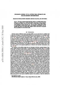
, where N = 1 and T1 = V . Viceversa, there exists a polynomial-time reduction algorithm that transforms any SPTP instance < G = (V, A, C), s, d, N, {Tk }k=1,...,N > into a single source - single destination SPP instance < G0 = (V 0 , A0 , C 0 ), s, d0 = d + (N − 1) · n >, where G0 is a multi-stage graph with N stages, each replicating G. Figure 2 depicts the pseudo-code of the reduction algorithm SPTPReduction that performs the following operations: i. (line 1) V 0 := {1, 2, . . . , N · n}; A0 := ∅; ii. (lines 2–6) at each iteration, an arc (a, b) is added to A0 . In particular, for each stage k ∈ {1, . . . , N − 1}, for each node v ∈ {1, . . . , n}, and for each adjacent node w ∈ F S(v), (a, b) = (v + (k − 1) · n, w + k · n) with length cvw , if w ∈ Tk+1 ; (a, b) = (v + (k − 1) · n, w + (k − 1) · n) with length cvw , otherwise. It is easy to see that |A0 | = N · m and therefore the computational complexity of SPTPReduction is TN O(N ·m). Note that, since k=1 Tk = ∅, it results that N ≤ n, and therefore, the worst case computational complexity is O(n · m). Figure 3 depicts the multi-stage graph G0 corresponding to the SPTP instance on the small graph G of Figure 2. Note that, |V 0 | = N · n = 4 · 7 = 28, |A0 | = N · m = 4 · 11 = 44, s = 1, d0 = d + (N − 1) · n = 7 + 3 · 7 = 28. We now claim that in G0 , as constructed above, there is a path P 0 from s to d0 of length K if and only if in G there is a path tour PT from s to d of length K. Suppose that in G0 there is a path P 0 of length K from s to d0 . Because P 0 connects s ∈ T1 to d0 ∈ TN , for each k = 1, . . . , N − 1 there must be in P 0 necessarily at least one arc connecting two nodes in consecutive stages k and k + 1. Therefore, it follows that P 0 consists of at least one node in each of the N stages, so corresponding to a path tour PT of length K in G that successively passes through at least one node from the given node subsets T1 , T2 , . . . , TN . 3
k=1 s 2
k=2
1
1
8
1
1
2
3
2
16
9 3
3
1
4
3
18
11
5
3
12
19
13
20 2
7
4 1
4
2
5
24
4
4
6
23 1
1
1
1 4
17
10 4
1
5
5
3
22
1
2 1
2
1
5
k=4
15
1
1
2
1
3
k=3
v’=v+(k−1)*n=1+(2−1)*7=8
4
4
25
26
3
3
27 2
2
21
14
d
28
L(SP)=11
Figure 3: The multi-stage graph G0 corresponding to the SPTP instance on G of Figure 2.
Viceversa, suppose that in G there is a path tour PT of length K that successively passes through at least one node from the given node subsets T1 , T2 , . . . , TN . Then, by construction, for each arc in PT connecting in G two nodes belonging to consecutive subsets, there exists in the simple path P 0 an arc connecting in G0 two nodes belonging to consecutive stages, till finally moving to d0 in the last stage N .
3
Several alternative algorithms
Once obtained in polynomial-time the multi-stage graph G0 , any shortest path algorithm can be applied to solve the resulting SPP. Although the huge number of state-of-the-art algorithms for the SPP, there does not exist a best method that outperforms all the others. In fact, recent research lines tend to develop techniques designed ad hoc for solving special structured shortest path problems: either a special network topology or a special cost structure. Exhaustive surveys of the most interesting and efficient shortest path algorithms, important for their computational time complexity or for their practical efficiency, can be found among others in [1], [8, 9, 7], [11], [10], [12], [14], and [17]. We have designed the following algorithms: • a dynamic programming algorithm, as suggested in [3]; • a Dijkstra like algorithm ([13]) that uses a binary heap to store the nodes with temporary labels; • several Auction like algorithms ([2, 4]): a forward, a backward, and a combined for/backward version. To describe the dynamic programming approach we will use a slight different notation to represent an expanded graph G0 = (V 0 , A0 , C 0 ). For each node i ∈ V , V 0 contains N + 1 nodes (i, 0), (i, 1), . . ., (i, N ). The meaning of being in node (i, k), k = 1, 2, . . . , N , is that we are at node i and have already successively visited the sets T1 , . . . , Tk , but not yet the sets Tk+1 , . . . , TN . The meaning of being in node (i, 0) is that we are at node i and have not yet visited any node in the set T1 . For each arc (i, j) ∈ A and for each k = 0, 1, . . . , N − 1, we 4
introduce in A0 an arc from (i, k) to (j, k), if j ∈ / Tk+1 or an arc from (i, k) to (j, k + 1), if j ∈ Tk+1 . Moreover, for each arc (i, j) ∈ A we introduce in A0 an arc from (i, N ) to (j, N ). Once obtained the expanded graph G0 , the SPTP is equivalent to find a shortest path from (s, 0) to (d, N ). Let Dr+1 (i, k), k = 0, 1, . . . , N , be the shortest distance from (i, k) to the destination node (d, N ) using r arcs or less. For k = 0, 1, . . . , N − 1 the DP iteration is the following: ( D r+1 (i, k)
=
D
r+1
(i, N )
min {cij + D (j, k),
(i,j)∈A
( =
) r
min
j ∈T / k+1
r
min {cij + D (j, k + 1)}
j∈Tk+1
(2)
r
min {cij + D (j, N )},
(i,j)∈A
0,
if i 6= d; if i = d.
Initial conditions are the following: ½ 0
D (i, k) =
∞, 0,
if (i, k) 6= (d, N ); if (i, k) = (d, N ).
Theorem 3 An algorithm implementing the above DP iteration terminates after a finite number of iterations with an optimal solution and its computational complexity is O(N 2 · n · m), and O(n3 · m) in the worst case. Proof: Given the nonnegativity of arc lengths, for each r and for each node (i, k), Dr+1 (i, k) ≤ Dr (i, k), since there are more candidate paths as the number of arcs increases. Moreover, a shortest path from node (i, k) to node (d, N ) that uses at most r + 1 arcs consists of an initial arc from (i, k) to node (j, l) (l ∈ {k, k + 1}) and a path P from (j, l) to (d, N ) that crosses at most r arcs. Obviously, DP iteration (2) follows from considering that P should be chosen as short as possible and its length is therefore Dr (j, l) and that node (j, l) should also be chosen in the most profitable way. Since there are no negative length cycles, there exists a shortest path having at most |V 0 | − 1 arcs, and therefore the number of needed iterations is at most |V 0 | = n · (N + 1). Finally, it can be easily seen that the computational complexity of an algorithm implementing the DP iteration (2) is O(N 2 · n · m), and O(n3 · m) in the worst case.
4
Experimental results and future work
In this section, we report on some preliminary computational experiments designed to determine which algorithm among those proposed seems to be more effective to solve the SPTP. The following algorithms have been implemented in C language and run on a Pentium 4 with 2400 Mhz and 512 Mb of RAM: • Dijkstra forward with binary heap; • standard Auction forward; • standard Auction backward; • combined for/backward Auction fb; • DP Dijkstra, DP with Dijkstra as initialization phase; • DP Auction, DP with Auction as initialization phase; • DP Dijkstra, DP with Dijkstra as initialization phase; • DP Auction back, DP with Auction backward as initialization phase; 5
Complete graphs with n=60
Rectangular grid graphs with n=25 x 6
0.3
0.35
Dijkstra Auction fb Auction forward Auction backward DP Auction DP Auction back DP Dijkstra DP Dijkstra back
0.25
Dijkstra Auction forward Auction backward DP Auction DP Auction back DP Dijkstra DP Dijkstra back
0.3
0.25
0.2
Time (sec.)
Time (sec.)
0.2
0.15
0.15
0.1
0.1 0.05
0.05
0
5
10
15
20
25
30
35
40
0
45
0
N
20
40
60
80
100
N
Random graphs with n=150 and m=4 x n
Random graphs with n=150 and m=8 x n
0.2
0.35
Dijkstra Auction forward Auction backward DP Auction DP Auction back DP Dijkstra DP Auction
0.18 0.16
Dijkstra Auction forward Auction backward DP Auction DP Auction back DP Dijkstra DP Auction
0.3
0.25
0.14
Time (sec.)
Time (sec.)
0.12 0.1 0.08 0.06
0.2
0.15
0.1
0.04
0.05
0.02 0
10
20
30
40
50
60
70
80
90
100
0
110
10
N
20
30
40
50
60
70
80
90
100
110
N
Figure 4: For each problem family, 10 different instances have been generated for each possible value of N ∈ {10%n, 30%n, 50%n, 70%n} and the mean time (in sec.) required to find an optimal solution has been stored and plot.
• DP Dijkstra back, DP with Dijkstra backward as initialization phase. The algorithm simply implementing DP iteration (2) has been also coded and it is has been revealed too time consuming and not very efficient. The algorithm can be made more efficient by observing that to calculate D(i, k) for all i, it is not needed to know D(i, k − 1), . . . , D(i, 0), but it is sufficient to know just D(j, k + 1) for j ∈ Tk+1 . Thus, we have calculated first D(i, N ) using a standard shortest path computation (DP Dijkstra, DP Auction, DP Dijkstra, DP Auction back, DP Dijkstra back). The algorithms above listed have been tested on the following graph families: 1) complete graphs with n ∈ {60, 100}; 2) square grids with n = 10 × 10 and rectangular grids with n = 25 × 6; 3) random graphs with n = 150 and m ∈ {4 × n, 8 × n}. For each problem family, 10 different instances have been generated for each possible value of N ∈ {10%n, 30%n, 50%n, 70%n} and the mean time (in sec.) required to find an optimal solution has been stored and plot in Figure 4. Looking at the preliminary results, it seems that Dijkstra’s algorithm outperforms all the competitors. Nevertheless, further experiments are needed on a wider set of instances and further investigation is planned in the next future in order to implement and test a collection of different algorithms by using path cost upper bounds, by mixing Auction and graph collapsing ([5]) and virtual sources ([6]) ideas. Moreover, it would be interesting to study some variants of the SPTP and TN their complexity where the constraint k=1 Tk = ∅ is relaxed and/or arc capacity constraints are added. 6
References [1] R.K. Ahuja, T.L. Magnanti, and J.B. Orlin. Network Flows: Theory, Algorithms and Applications. Prentice-Hall Englewood Cliffs, 1993. [2] D.P. Bertsekas. An auction algorithm for shortest paths. SIAM Journal on Optimization, 1:425–447, 1991. [3] D.P. Bertsekas. Dynamic Programming and Optimal Control. 3rd Edition, volume I. Athena Scientific, 2005. [4] D.P. Bertsekas, S. Pallottino, and M.G. Scutell`a. Polynomial auction algorithms for shortest paths. Computational Optimization and Application, 4:99–125, 1995. [5] R. Cerulli, P. Festa, and G. Raiconi. Graph collapsing in shortest path auction algorithms. Computational Optimization and Applications, 18:199–220, 2001. [6] R. Cerulli, P. Festa, and G. Raiconi. Shortest path auction algorithm without contractions using virtual source concept. Computational Optimization and Applications, 26(2):191–208, 2003. [7] B.V. Cherkassky and A.V. Goldberg. Negative-cycle detection algorithms. Mathematical Programming, 85:277–311, 1999. [8] B.V. Cherkassky, A.V. Goldberg, and T. Radzik. Shortest path algorithms: Theory and experimental evaluation. Mathematical Programming, 73:129–174, 1996. [9] B.V. Cherkassky, A.V. Goldberg, and C. Silverstein. Buckets, heaps, lists, and monotone priority queues. SIAM Journal of Computing, 28:1326–1346, 1999. [10] E.V. Denardo and B.L. Fox. Shortest route methods: 2. group knapsacks, expanded networks, and branch-and-bound. Operational Research, 27:548–566, 1979. [11] E.V. Denardo and B.L. Fox. Shortest route methods: reaching pruning, and buckets. Operational Research, 27:161–186, 1979. [12] N. Deo and C. Pang. Shortest path algorithms: taxonomy and annotation. Networks, 14:275–323, 1984. [13] E. Dijkstra. A note on two problems in connexion with graphs. Numer. Math., 1:269–271, 1959. [14] G. Gallo and S. Pallottino. Shortest path methods: A unified approach. Math. Programming Study, 26:38–64, 1986. [15] R.M. Karp. Reducibility among combinatorial problems. In R.E. Miller and J.W. Thatcher, editors, Complexity of Computer Computations. Plenum Press, 1972. [16] C.H. Papadimitriou and K. Steiglitz. Prentice-Hall, 1982.
Combinatorial optimization: Algorithms and complexity.
[17] D.R. Shier and C. Witzgall. Properties of labeling methods for determining shortest path trees. Journals of Research of the National Bureau of Standards, 86:317–330, 1981.
7