We show that, with careful socket buffer sizing, a bulk TCP transfer can saturate .... that the transfer is congestion-limited; otherwise, if the send- window is limited ...
1
The TCP Bandwidth-Delay Product revisited: network buffering, cross traffic, and socket buffer auto-sizing Manish Jain, Ravi S. Prasad, Constantinos Dovrolis Networking and Telecommunications Group College of Computing Georgia Tech jain,ravi,dovrolis @cc.gatech.edu �
Abstract— TCP is often blamed that it cannot use efficiently network paths with high Bandwidth-Delay Product (BDP). The BDP is of fundamental importance because it determines the required socket buffer size for maximum throughput. In this paper, we re-examine the BDP concept, considering the effects of network buffering and cross traffic on the ‘bandwidth’ and ‘delay’ characteristics of a path. We show that, with careful socket buffer sizing, a bulk TCP transfer can saturate a network path independent of the BDP or the available network buffers. In a non-congested path, there is a certain socket buffer size (which depends on the cross traffic type) that maximizes the throughput of a bulk TCP transfer. In a congested path, the TCP throughput is maximized when the connection is limited by the congestion window, rather than by the socket buffers. Finally, we present an application-layer mechanism (SOBAS) that automatically adjusts the socket buffer size close to its optimal value, based on direct measurements of the maximum received throughput and of the round-trip time, without requiring prior knowledge of the path characteristics. Keywords: TCP throughput, router buffers, available bandwidth, bottleneck bandwidth, round-trip time, fast longdistance networks. I. I NTRODUCTION There is a significant interest recently in end-to-end performance over high-bandwidth and long-distance networks [1]. In particular, it is the scientific community that pushes the edge of network performance with applications such as distributed simulation, remote colaboratories, and with huge transfers (gigabytes or more). Typically, such applications run over well-provisioned networks (Internet2, ESnet, GEANT, etc) built with high-bandwidth links (OC-12 or higher) that are lightly loaded in most of the time. Additionally, through the gradual deployment of Gigabit Ethernet inThis work was supported by the ‘Scientific Discovery through Advanced Computing’ program of the US Department of Energy (award number: DE-FC02-01ER25467), and by the ‘Strategic Technologies for the Internet’ program of the US National Science Foundation (award number: 0230841). Please do not distribute without the authors’ permission.
terfaces, congestion also becomes rare at the network edges and end-hosts. With all this network bandwidth, it is not surprising that users expect a superb end-to-end performance. However, this is not always the case. A recent measurement study at the Internet2 showed that 90% of the ‘bulk’ TCP transfers (i.e., transfers of more than 10MB) typically receive less than 5Mbps [2]. This is an unsatisfactory result, given that Internet2 uses OC-48 links that are rarely utilized by more than 30%, while most universities connected to Internet2 also operate high-bandwidth and well-provisioned networks. A popular belief is that a major reason for the relatively low end-to-end throughput in fast long-distance networks is TCP. This is either due to TCP itself (e.g., its congestion control algorithms and parameters), or because of local system configuration (e.g., default TCP socket buffer size) [3], [4].1 TCP is blamed that it is slow in capturing the available bandwidth of high-performance networks, especially in transfers over long-distance paths. Two issues commonly identified as the underlying reasons are: 1. Limited socket buffers at the TCP sender or receiver impose a conservative upper bound on the effective window of the transfer, and thus on the maximum achievable throughput. 2. Packet losses cause a large and multiplicative window reduction, and a subsequent slow (linear) window increase rate, causing an overall low average throughput. Other TCP-related issues that often impede performance are multiple packet losses at the end of slow-start (commonly resulting in timeouts), the inability to distinguish between congestion and random packet losses, the use of small segments, the coarse granularity of the retransmission timeout, or the initial value of the ssthresh parameter [5], [6]. Networking research has focused on these problems, pursuing mostly three approaches: modified congestion control algorithms [7], [8], [9], [10], parallel TCP transfers [11], [12], [13], [14], and improved socket buffer sizing [5], [15], [16], [17]. Modified congestion control schemes, possibly �
Other reasons include Fast Ethernet duplex mismatches, lossy cables, under-buffered switches/routers, and poorly written applications.
2
with cooperation from routers [9], can lead to significant benefits for both applications and networks, and they can also address other important issues, such as the detection of congestion unresponsive traffic. Modifying TCP, however, is an enormously difficult task today, given the millions of existing TCP installations and the fairness issues that would arise during deployment of diverse congestion control algorithms. Parallel TCP connections can increase the aggregate throughput that an application receives. They also raise fairness issues, however, because an aggregate of connections decreases its aggregate window by a factor ���� , rather than �� , upon a packet loss. Also, the aggregate window increase rate is times faster than that of a single connection. This paper follows the socket buffer sizing approach, rather than modifying TCP or using parallel connections. Socket buffer sizing can be performed by applications, and so it does not require changes at the TCP implementation or protocol. Also, it is a mechanism that can work complementary with parallel connections. Even if TCP evolves to a different protocol in the future, we believe that it is still important to consider how we can improve application performance in the shorter term, using the existing TCP incarnation. How can an application determine an appropriate size for the socket buffer at the sender and receiver of a TCP transfer? A first constraint is that the socket buffers cannot exceed the memory that the operating system makes available for that connection. Throughout the paper, we assume that the end-hosts have enough memory and that this constraint is met. This is widely the case today, with the exception perhaps of busy Web or file servers. A second constraint is that the two socket buffers, or actually the smaller of the two, should be sufficiently large so that the transfer can saturate the underlying network path. This leads us to a fundamental concept in any window-controlled transport protocol: the Bandwidth-Delay Product (BDP). Specifically, suppose that the bottleneck link of a path has a transmission capacity (‘bandwidth’) of � bps and the path between the sender and the receiver has a Round-Trip Time (RTT) of � sec. The connection will be able to saturate the path, achieving the maximum possible throughput � , if its effective window is ��� � . This product is historically referred to as BDP. For the effective window to be � ��� , however, the smaller of the two socket buffers should be equally large. If the size of that socket buffer is less than � � � , the connection will underutilize the path. If it is more than ��� � , the connection will overload the path, and depending on the amount of network buffering, it will cause congestion, packet losses, window reductions, and possibly throughput drops. The previous interpretation of the BDP, and its relation to TCP throughput and socket buffer sizing, are well-known in the networking literature. As we argue in Section II, however, the socket buffer size should be equal to the BDP only in the case of a path that does not carry competing traffic
(‘cross traffic’) and that does not introduce queueing delays. The presence of cross traffic means that the ‘bandwidth’ of a path will not be � , but somewhat less than that. Also, packet buffers in the network routers can cause queueing delays, meaning that the RTT of the path will be larger than the fixed delay � . Given these two additional effects (cross traffic load, and queueing delays), how should we define the BDP of a network path? Should we interpret the ‘bandwidth’ term of the BDP as the capacity � , the available bandwidth which remains unclaimed from cross traffic, the ‘fair share’ in the path (for some definition of fairness), or as something different than the above? And how should we interpret the ‘delay’ term of the BDP? Is it the minimum possible RTT, the average RTT before the TCP connection starts (including queueing delays due to cross traffic), or the average RTT after the TCP connection starts? In Section III, we review the previous work in the area of socket buffer sizing, arguing that the BDP has been given different interpretations in the past and that it is still unclear what is the socket buffer size that maximizes the throughput of a bulk TCP transfer. The first objective of this paper is to examine the effects of the socket buffer size, the amount of network buffering, and the cross traffic type on the throughput of a bulk TCP transfer. In Section IV, we focus on the effect of network buffering. We show that, with appropriate socket buffer sizing, a TCP transfer can saturate a network path, independent of how large the BDP is, and independent of the available network buffering. In Sections V and VI, we examine the effects of cross traffic on the TCP throughput. The type of cross traffic is crucial, as it determines whether and by how much the latter will decrease its send-rate upon the initiation of a new TCP transfer. We identify four distinct common types of cross traffic: rate-controlled UDP flows, TCP transfers limited by congestion, TCP transfers limited by socket buffers, and TCP transfers limited by size. We show that, depending on the cross traffic type, the Maximum Feasible Throughput of a TCP connection can be the Available Bandwidth [18], the Bulk Transfer Capacity (BTC) [19], or the maximum TCP throughput that does not cause packet losses in the path. An important conclusion from Sections V and VI is that, independent of cross traffic and network buffering, there is a certain socket buffer size that maximizes the throughput of a bulk TCP transfer. The second objective of this paper is to develop an application-layer mechanism that can automatically set the socket buffer size so that the TCP transfer receives its Maximum Feasible Throughput, or at least close to that. In Section VII, we describe the proposed SOcket Buffer AutoSizing (SOBAS) mechanism. SOBAS estimates the path’s BDP from the maximum TCP goodput measured by the receiving application, as well as from out-of-band RTT measurements. We emphasize that SOBAS does not require changes in TCP, and that it can be integrated in principle
3
with any TCP-based bulk data transfer application. SOBAS has been evaluated through simulations and Internet experiments. Simulations are used to compare SOBAS with the Maximum Feasible Throughput and with other socket buffer sizing techniques under the same traffic conditions. Experimental results provide us with confidence that SOBAS works well, even with all the additional measurement inaccuracies, traffic dynamics, non-stationarities, and noise sources of a real Internet path. A key point about SOBAS is that it does not require prior knowledge or estimation of path characteristics such as the end-to-end capacity or available bandwidth. We conclude in Section VIII. II. W HAT
BANDWIDTH -D ELAY P RODUCT
DOES
MEAN ?
Consider a unidirectional TCP transfer from a sender ��� � ��� � . TCP is window-controlled, meanto �� a� receiver �
ing that is allowed to have up to a certain number of transmitted but unacknowledged bytes, referred to as the send-window � , at any time. The send-window is limited by (1)
�� ������ � ����� ������ ��� where � is the sender’s congestion window [20], � is the receive-window advertised��by �� ���!� , and � � is the size of the send-socket buffer at . The receive-window � is the amount of available receive-socket buffer memory at ��� � , and is limited by the receive-socket buffer size �"� , i.e., ���#$�%� . So, the send-window of a transfer is limited by: (2)
�� &�'�(�)� ����* � where * +�'�(�)� �"�,��� � � is the minimum of the two socket buffer sizes. If the send-window is limited by -� , we say that the transfer is congestion-limited; otherwise, if the sendwindow is limited by * , we say that the transfer is bufferlimited. A transfer can be congestion-limited or bufferlimited at different time periods. If �/.0 �21 is the connection’s RTT when the send-window is � , the transfer’s throughput is
3
� �(�!� �4�5* � '
�
� .0 �21 / �/.6 �21
(3)
Note that the RTT can vary with � because of queueing delays due to the transfer itself. We next describe a model for the network path 7 that the TCP transfer goes through. The bulk TCP transfer that we focus on is referred to as the target transfer; the rest of the traffic in the path ��� � is referred to as cross traffic. The forward path from to ���!� , and the reverse path from ���!� to ���� , are assumed to be fixed and unique for the duration of the target transfer. Each link 8 of the forward/reverse path transmits packets with a capacity of ��9 bps, causes a fixed delay :�9 , and it has link buffers that can store �"9 packets. Arriving packets are discarded in a Drop-Tail manner when the
corresponding buffer is full. The minimum RTT of the path is the sum of all fixed delays along the path �); =< 9?>�@ :49 . Also, let AB9 be the initial average utilization of link 8 , i.e., the utilization at link 8 prior to the target transfer. The available bandwidth CD9 of link 8 is then defined as CD9 � 9 �-.FEHG A 9 1 . Due to cross traffic, link 8 introduces queueing delays together with the fixed delay :,9 . Let :�I 9KJL:49 be the average delay at link 8 , considering both fixed and queueing delays, prior to the target transfer. The exogenous RTT of the path is the sum of all average delays along the path �!M < 9N>�@ :�I 9 before the target transfer starts. Adopting the terminology of [18], we refer to the link of the forward path 7�O with the minimum capacity � �'��� @QP � �R9 � as the narrow link, and to the link with the minimum available bandwidth C &�'��� @ P � CD9 � as the tight link. We say that a link is saturated when its utilization is 100% (i.e., CD9 =0), and that it is congested when it drops packets due to buffer overflow (i.e., non-zero loss rate). Note that a link can be saturated but not congested, or congested but not saturated. We assume that the only saturated and/or congested link in the forward path is the tight link. A path is called congested or saturated, if its tight link is congested or saturated, respectively. The narrow link limits the maximum throughput � that the target transfer can get. The tight link, on the other hand, is the link that becomes saturated and/or congested after the target transfer starts, when the latter has a sufficiently large send-window. The buffer size of the tight link is denoted by �DS , while �DT S�#U�DS is the average available buffer size at the tight link prior to the target transfer. We refer to � , � ; , and � S as the structural path characteristics, and to C , �!M , and �H T S as the dynamic path characteristics prior to the target transfer. The dynamic path characteristics depend on the cross traffic. Equation (3) shows that the throughput of the target transfer depends on the 3 minimum socket 3 buffer size * . If we view the throughput as a function .0* 1 , an important question is: given a network path 7 , with certain structural and dynamic characteristics, for what value(s)3 of the socket buffer size V* the target transfer throughput .6* 1 is 3maximized? We refer to the maximum value of the function .6* 1 as the 3 Maximum Feasible Throughput (MFT) V . The conventional wisdom, as expressed in networking textbooks [21], operational handouts [4], and research papers [16], is that the socket buffer size * should be equal to the Bandwidth-Delay Product of the path, where ‘bandwidth’ is the capacity of the path � , and ‘delay’ is the minimum RTT of the path � ; , i.e., * � � � ; . Indeed, if the send-window is � � � � ; , and assuming that there is no cross traffic in the path, the tight link becomes saturated but not congested, and the 3 target transfer achieves its Maximum Feasible Throughput V � . Thus, in the case of no cross traffic, V* � � � ; . In practice, a network path always carries some cross traf-
4
�
� . If the socket buffer size is set to � � �); , fic, and thus C the target transfer will saturate the tight link, and depending on the number of buffers at the tight link �%S , it may also cause congestion. Congestion, however, causes multiplicative drops in the target transfer’s send-window, and, potentially, throughput reductions as well. Thus, the amount of buffering �DS at the tight link is an important factor for socket buffer sizing, as it determines the point at which the tight link becomes congested. The presence of cross traffic has two additional implications. First, cross traffic causes queueing delays in the path, and thus the initial RTT of the target transfer becomes the exogenous RTT � M , rather than the minimum RTT � ; . With larger � S and with burstier cross traffic, the difference between �!; and �!M becomes more significant. Second, if the cross traffic is TCP (or TCP-friendly), it will react to the initiation of the target TCP transfer reducing its throughput, either because of packet losses, or because the target transfer has increased the RTT in the path. Thus, the target transfer can achieve a higher throughput than what was the initial available bandwidth C . In the next section, we review the previous work in the area of socket buffer sizing, and identify several interpretations that have been given to the BDP: 1. BDP : * � � � ; � 2. BDP � : * � � �!M 3. BDP : * C � � ; 4. BDP : * C � �!M 5. BDP : * BTC � � � 6. BDP : * * (where *
�� ) The first four BDP definitions should be clear from the previous model. The bandwidth term in BDP is the Bulk Transfer Capacity (BTC), i.e., the average throughput of a bulk congestion-limited TCP transfer [22]. It can be argued that the BTC is the ‘fair-share’ of the target transfer in the path, according to TCP’s bandwidth sharing properties. � is the average RTT of the path, after the target transfer has started, and so it includes the queueing load due to the target transfer. BTC is determined by the congestion window and the average RTT of the target transfer, and so BDP is related to the average congestion window of the transfer. In BDP , * is set to a sufficiently large value, so that it is always larger than the congestion window. So, the meaning of BDP is that connection should be always congestionlimited. Of course, in the absence of any previous information about the path, it is hard to know how large the maximum congestion window will be. Note that BDP and BDP are different: in the former, the connection may be buffer-limited during parts of its lifetime, while in the latter the connection’s send-window is never limited by the socket buffers.
�
� � �
��
��
�� ��
�
��
�
�
�
III. P REVIOUS
�
�
WORK ON SOCKET BUFFER SIZING
There are several measurement and estimation techniques for bandwidth-related metrics, such as the capacity, available
bandwidth, or Bulk Transfer Capacity of a path [18], [22], [23], [24]. An application of such techniques is that they can be used to estimate the bandwidth term of a path’s BDP. An auto-tuning technique that is based on active bandwidth estimation is the Work Around Daemon (WAD) [5]. WAD uses ping to measure the minimum RTT �); prior to the start of a TCP connection, and pipechar to estimate the capacity � of the path [25]. In other words, [5] attempts to set the socket buffer size as in BDP . A similar approach � is taken by the NLANR Auto-Tuning FTP implementation [26]. In that work, however, the socket buffer sizing is based on the median, rather than the minimum, of the bandwidthdelay product measurements and so it is closer to BDP � . Similar BDP interpretations are given at the manual socket buffer sizing guidelines of [4] and [15]. A different bandwidth metric is considered in [27]. That work proposes a TCP variant in which the send-window is adjusted based on the available bandwidth of a path. The proposed protocol is called TCP-Low Priority (TCP-LP), and it is able to utilize any excess network bandwidth that would not be used normally by the regular TCP workload [27]. Even though TCP-LP is not a socket buffer sizing scheme, it relates more to BDP or BDP because it is the available bandwidth, rather than the capacity, that limits the transfer’s send-window. The first proposal for automatic TCP buffer tuning was [16]. The goal of that work was to allow a host (typically a server) to fairly share kernel memory between multiple ongoing connections. The proposed mechanism, even though simple to implement, requires changes in the operating system. An important point about [16] is that the BDP of a path was estimated based on the congestion window (cwnd) of the TCP connection. Thus, the socket buffer sizing objective in that work was similar to BDP . The receive-socket buffer size was set to a sufficiently large value so that it does not limit the transfer’s throughput. An application-based socket buffer auto-tuning technique, called Dynamic Right-Sizing (DRS), has been proposed in [17]. DRS measures the RTT of the path prior to the start of the connection (exogenous RTT). To estimate the bandwidth of the path, DRS measures the average throughput at the receiving side of the application. It is important to note however, that the target transfer throughput does not only depend on the congestion window, but also on the current socket buffer size. Thus, DRS will not be able to estimate in general the socket buffer size that maximizes the target transfer’s throughput, as it may be limited by the current socket buffer size. The socket buffer sizing objective of DRS does not correspond to one of the BDP definitions in the previous section. A comparison of some socket buffer sizing mechanisms is made in [28]. We finally note that the latest stable version of the Linux kernel (2.4) uses a non-standardized socket buffer sizing al-
�
�
�
5
gorithm. In particular, even if the application has specified a large receive-socket buffer size (using the setsockopt system call), the TCP receiver advertizes a small receive-window that increases gradually with every ACKed segment. It also appears that Linux 2.4 adjusts the send-socket buffer size dynamically, based on the available system memory and the transfer’s send-socket buffer backlog. IV. U NDER - BUFFERED
AND OVER - BUFFERED PATHS
Let us first examine the effect of network buffering on the throughput of a bulk TCP transfer, in the simple case of a path that does not carry cross traffic. 3 Consider the model of II. What is the average throughput .0* 1 of a bulk TCP transfer, as a function of the socket buffer size * , the path capacity � , the minimum RTT �!; , and the tight link buffer size �DS ? The following result, proven in Appendix-1, shows that we need to consider two cases, depending on the network buffering �%S . If �
S
is less than BDP , i.e., if � �
��� ��
.0* 1
� �
� ��� ��
3
S
�
�
��
��
,
if *
�
��
��
;
if �
� � �
;
#
;
� �
; &* # � S
�
� �
� ����� � �
�� ������� ��� ��� � ���
������ ���
�
if *
;
� �
� S
(4) When * is less than � � � ; , the connection is bufferlimited and it 3 does not saturate the path. As * increases, the throughput .0* 1 increases linearly until * becomes large enough ( � � ; ) to saturate the path. If * is sufficiently large to saturate the path, but without causing congestion, i.e., � � ; &* # � � ;� � S , the transfer achieves its Maximum 3 Feasible Throughput V , that is equal to the capacity � . For a larger socket buffer size ( * � �!; �HS ), the transfer causes packet losses at the tight link, and it becomes congestionlimited. Its throughput then depends on the amount of net� �Q; , the transfer cannot satuwork buffering �%S . If �DS rate the path when * � �!; �DS because the ‘sawtooth’ variations of the congestion window also cause throughput reductions. In other words, the transfer’s backlog at the tight link is not enough to absorb the loss-induced reduction of the transfer’s send-rate. When �%S � �Q; , we say that the path is under-buffered for the target TCP transfer. The resulting 3 throughput .0* 1 depends on the number of dropped packets each time the tight link buffer overflows; the expression in (4) assumes single packet losses. In the extreme case that �HS���� , the target transfer can only achieve 75% utilization of the tight link.
�
On the other hand, if �%S�J saturate the path even if *
; the target transfer can � � ; � S , assuming again
�
� �
single packet losses:
3
.0* 1
�
� ��� � � �
if * if *
#
� �
;
� �
;
(5)
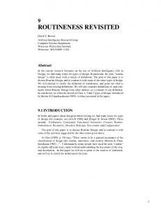
The important difference in this case is that losses, and the subsequent send-window reductions, do not decrease the transfer’s throughput. This is because the transfer’s backlog at the tight link is sufficiently large to keep that link saturated while the send-rate is less than � . When �%S � � ; , we say that the path is over-buffered for the target transfer. Note that whether the path is under-buffered or overbuffered depends on the target transfer’s RTT �! . If the network operator provisions the network buffer size as �"S � � �" based on the RTT �� , the path will be under-buffered for connections with larger RTT, and over-buffered for connections with smaller RTTs. The previous result also shows why TCP often performs inefficiently in high bandwidth-delay product paths. Such paths require significant amounts of network buffering at each router/switch interface that may become the tight link of the transfer. The required buffering is at least ��� �! in terms of bytes, or at least �� in terms of seconds. If the interface buffers are dimensioned based on open-loop (non-TCP) traffic, such as in [29], the path can be significantly underbuffered for most TCP traffic. For this reason, some network providers install hundreds of msec worth of buffering in their router interfaces. Large amounts of network buffering, however, can also cause large queueing delays and jitter, affecting the performance of real-time and streaming applications. Sometimes applications set their socket buffer size to the largest possible value that the operating system allows, in an attempt to maximize the resulting throughput. In that case, however, the transfer may become congestion-limited. Then, if the path is under-buffered for that transfer, the latter will not manage to saturate the path. Even if the path is overbuffered, the target transfer may not be able to get its Maximum Feasible Throughput when it loses several packets at a congestion event.2 Equations (4) and (5), however, show an important and positive point that we should focus on: a TCP transfer can achieve its Maximum Feasible Throughput independent of the network buffering �%S , as long as the socket buffer size is *+#�� � ;# � S . That range limited in the range � � ; results in path saturation, but without congestion. To operate at that ‘sweet spot’, the socket buffer size * must be chosen based on the bandwidth and RTT characteristics of the path, rather than to be blindly set to its maximum possible value. To illustrate this point, Figure 1 shows the goodput of two successive 1-gigabyte transfer from host bwest.cc.gt.atl.ga.us to host nyu.ron.lcs.mit.edu. The BDP $
�
Bursty losses are quite common in Drop-Tail buffers [30].
6
types of cross traffic, they represent three distinct and major points in the congestion responsiveness space.
GaTech to NYU Receive Socket Buffer: 470KB 100 80
Reverse path sources
Sink
40 20 SND
0
10
20
30
40
50
60
70
80
Tight link
10 msec
RCV
1Gbps
90
50 Mbps, 40ms
ms
bp
s, 1
0m
s
2 persistent TCP sources per node 1 ... 10
1 ... 10 1 2 ... 10
40 20
Sink
s m
60
bp
10
1G
s,
1G
80
1 pareto UDP source per node
200 size−limited TCP sources per node
Fig. 2. Simple simulation topology. 0
10
20
30
40
50
60 70 80 Time (sec)
90 100 110 120 130 140
Fig. 1. Throughput of 1-gigabyte transfer with two socket buffer sizes.
of this path is 436KB3 , with a layer-2 capacity of 100Mbps. In the top transfer of Figure 1, the receive-socket buffer size (which is smaller than the send-socket buffer size) is 470KB. With this value of * , the transfer does not experience any packet losses, and its goodput is about 91.3Mbps, close to the capacity of this path. On the other hand, in the bottom transfer of Figure 1, the receive-socket buffer size is set to 950KB, and the transfer receives an average goodput of only 61.7Mbps. The reason is that with the larger socket buffer size, the transfer overloads the network buffers, causing (bursty) packet losses, and subsequent large window reductions. This experiment illustrates that a limited socket buffer size can improve the throughput of a TCP transfer, when it is large enough to saturate the path, but not so large that it would cause congestion. V. MFT
AT A NON - CONGESTED PATH
In this section, we consider a path that is not congested (i.e., no packet losses at tight link) prior to the target TCP transfer. Our objective is to examine the relation between the 3 throughput .6* 1 of the target transfer and its socket buffer size * , and to identify the Maximum Feasible Throughput for different types of cross traffic. This throughput of the target transfer depends on the congestion responsiveness of cross traffic, i.e., the way in which the throughput of cross traffic flows is reduced after the start of the target transfer. We consider three types of cross traffic in a non-congested path: 1. Rate-controlled UDP sources with constant average rate. 2. Buffer-limited persistent TCP transfers (‘elephants’). 3. Size-limited short TCP transfers (‘mice’). As will be shown next, the previous traffic types are fundamentally different in terms of their congestion responsiveness. Even though we do not claim that these are the only Throughout the paper, KB means 1000 bytes.
The following results are illustrated with NS simulations. The simulated network is shown in Figure 24 . All data packets are 1000 bytes long. The structural path characteristics are � =50Mbps, �!; =100msec, and so � � ; =625,000 bytes or 625 data packets. For each cross traffic type, we simulate three tight link buffer sizes � S : �� � � ; =313 packets (under-buffered), � � ; =625 packets, (well-buffered), and � �Q; =1250 packets (over-buffered). Depending on the type of cross traffic that we consider next, some of the sources shown in Figure 2 are turned off. The reverse path carries the same cross traffic as the forward path. �
A. Cross traffic with constant average rate Suppose that the tight link of the path carries only rate3 � S . controlled cross traffic, with constant average rate � This type of cross traffic will not adapt its send-rate after the target TCP transfer starts, independent of any losses or queueing delays in the path. For this reason, we also refer to it as congestion unresponsive. The dynamic characteristics of the path, prior to the target transfer, need to include the additional load, average queueing delay, and buffer occupancy that the cross traffic causes in the tight link of the �
We use this simplistic topology here to isolate the cross traffic type from more complex effects that can appear in a multihop topology. A more complex network is simulated in VII. �
18 16
TCP throughput (Mbps)
0
1G
, 10 s bps , 10m s
Receive Socket Buffer: 950KB 100
1Gb ps, 2 m 1Gbps, 4m s s 20ms 1Gbps,
0
bp 1G
TCP throughput (Mbps)
60
14 12 10 8 Available bandwidth Link Buffer = 313 pkts Link Buffer = 625 pkts Link Buffer = 1250 pkts
6 4 2
0
50
100 150 200 250 300 350 400 450 500 550 600 650 Socket buffer size (pkts)
Fig. 3. Cross traffic: rate-controlled UDP (constant average rate).
7
3
��
40 35
TCP throughput (Mbps)
�, path. Specifically, the available bandwidth is C � G the average exogenous RTT is �)M J � ; , and the average available buffer space at the tight link is �DT S #&�DS . As a first-order approximation, we assume a fluid model for both the cross traffic and the target transfer. Under this assumption, the dynamic characteristics of the path become constant. Following the same derivations as in Appendix-1, the throughput of the target transfer would be then given by Equations (4) and (5), replacing � by C , � ; by � M , and � S by � T S . So, the path would be over-buffered if � T S J&C 3 � M , and in that case the target transfer throughput would be .0* 1 3 *� �!M if * #&C �!M , and .0* 1 C if * &C �)M . If the path is under-buffered � (i.e., � T S &C � � M ), the throughput will drop to �� . � T S C � M 1 ���. � T S C � M 1 G � T S C � M�� when * &C � M� 3 �HT S . So, when the cross traffic has a constant average rate � , the MFT of the target 3 3 transfer is the available bandwidth C , i.e., V C �$G � . Also, the optimal socket buffer size V* would be any value in � C � M � C � M� � T S�� . Because of traffic burstiness however, a backlog will be C ��M , and packet created at the tight link even when * losses can occur even when * &C �)M �HT S . As the network buffering �DS decreases, the deviations between the fluid traffic model and bursty traffic would be larger. So, the MFT in practice can be less than C , especially in paths with inadequate network buffering. For the same reason, the optimal socket buffer size in practice would be closer to V* C �!M (empty buffer) rather than to C � M� � T S (full buffer). 3 Figure 3 shows the target transfer throughput .6* 1 , for three network buffering levels, as a function of the socket buffer size * . The cross traffic is generated from 10 sources with Pareto distributed packet interarrivals (scale parameter � =1.5). The tight link utilization is 70% initially (C =15Mbps), and the exogenous RTT is 102ms. According to the previous model, the optimal socket buffer size would be V* C � M =191pkts. When �DS =1250pkts, we see 3 that the target transfer can saturate the path ( V =15Mbps, V* =250-350pkts). For lower network buffering (625pkts and 313pkts), the target transfer has a lower MFT (14.5Mbps and 12Mbps), and a smaller optimal socket buffer size (250pkts and 150pkts) because the tight link buffers overflow before that link is saturated. In summary, when the cross traffic consists of congestion unresponsive flows with constant average rate, the MFT of the target TCP transfer can be up to the initial available bandwidth C . Suppose that the cross traffic is generated from a persistent and buffer-limited TCP transfer with maximum window -�0S and RTT �!�0S . Since the transfer is buffer-limited, it does not 3 create congestion in the path, and its throughput is �0S
�0S � �0S # � . In the following derivations, we assume again a fluid traf-
25 20 15 Available bandwidth Link Buffer = 313 pkts Link Buffer = 625 pkts Link Buffer = 1250 pkts
10 5 0
B. Buffer-limited TCP transfers
30
200
400
800 1000 600 Socket buffer size (pkts)
1200
1400
Fig. 4. Cross traffic: buffer-limited persistent TCP transfers.
fic model. Before the target TCP3 transfer starts, the available bandwidth in the path is C = � G �0S J 0, the exogenous RTT is �!M , and the available tight link buffer space is �DT S #��HS . If the target transfer’s socket 3 buffer size is * # C ��M , it will not saturate the path, 3 and .6* 1 *� � 3 M # C . If however C �!M * # ; �!M �HT S , where ; is the maximum target transfer throughput for which there are no packet losses at the tight link (will be derived later), the target transfer the tight link and � will saturate � it will create a backlog 3
* G .0* 1 �!M . The backlog will� increase the RTT of the cross traffic transfer to � �0 S �!�0S � . The window of that transfer is limited to �0S however, and so its throughput will be now reduced to
�
3
�0S
!�0S �
�0S �
�
�
.� G C 1
�0S �
�
�0S �
3 �
�0S
(6)
Thus, the target transfer’s throughput will be
3
.0* 1 �
G
3
� � 2C 0� S C �0S" � J C � � � �
(7)
which means that the target transfer received some of the bandwidth that was previously utilized by the cross traffic transfer. The MFT of the target transfer is achieved when the latter fills up the available buffer at the tight link, but without causing packet losses,
3
V C
� �0S" �� C 0� S" � T S C #�C �!�0S �� � �!�0S �D T S� � �
3
(8)
V � M �T S. and so the optimal socket buffer size is V* Also note that the maximum lossless throughput of the target 3 transfer ; � is equal to the MFT. 3 Figure 4 shows the target transfer throughput .0* 1 , for three network buffering levels, as a function of the socket buffer size. The buffer-limited persistent transfers are generated from 20 TCP Reno sources. The average RTT of the cross-traffic transfers is 100msec, and their maximum window size is 22 packets so that they create a tight link
�
8
20 18
buffer size. The mice are generated from 2000 TCP Reno sources (200 at each of 10 nodes) that transfer 10-15 data packets, and then they ‘sleep’ for a time interval before starting a new TCP connection. is uniformly distributed between 4.25 to 4.75 seconds here to achieve a 70% utilization at the tight link (C =15Mbps). 3 Note that the throughput function .6* 1 is similar, in shape, with the corresponding function of buffer-limited cross traffic in Figure 4: 3 1) .0* 1 increases linearly with * up to C , until the target transfer saturates the path (if the path is adequately buffered), 3 3 2) then, .0* 1 increases sublinearly with * up to the MFT V , as the target transfer accumulates backlog at the tight link, increasing the mice’s RTT and decreasing their throughput, 3) finally, the target transfer causes packet losses at the tight link, becomes congestion-limited, and its throughput drops to the BTC. A major difference between mice and elephants, however, is that the MFT with the former cross traffic type is much lower: 14.5Mbps ( �DS =313pkts), 16Mbps (�%S =625pkts), and 19.5Mbps (�DS =1250pkts); the corresponding MFT values for elephants were 24Mbps, 29Mbps, and 36Mbps. The MFTs with mice cross traffic are close to the available bandwidth (C =15Mbps), which is generally the case with congestion unresponsive cross traffic. Actually, in the extreme case where the size of each mouse is only a single packet, the aggregate of many mice entering the network with a constant arrival rate would be strictly congestion unresponsive. In summary, size-limited TCP transfers behave, in terms of their congestion responsiveness, somewhere between buffer-limited persistent TCP transfers and rate-controlled UDP flows: they react individually to losses and increased RTTs, but as an aggregate they do not share much of the bandwidth that they already possess. The MFT with sizelimited TCP cross traffic results (as in the case of bufferlimited TCP cross traffic) from the maximum socket buffer size that does not cause packet losses at the tight link. �
16
TCP throughput (Mbps)
�
14 12 10 8 Available bandwidth Link Buffer = 313 pkts Link Buffer = 625 pkts Link Buffer = 1250 pkts
6 4 2 0
0
50
100 150 200 250 300 350 400 450 500 550 600 650 Socket buffer size (pkts)
Fig. 5. Cross traffic: size-limited short TCP transfers.
utilization of 70% (C =15Mbps). The measured MFTs are: 24Mbps (�DS =313pkts), 29Mbps (�%S =625pkts), and 36Mbps (� S =1250pkts). The corresponding MFTs from Equation (8) are 27Mbps, 32Mbps, and 38Mbps. As in V-A, the model overestimates the MFT and the optimal socket buffer size, because it assumes that losses occur only when the tight link is saturated and the average available buffer space is zero. In summary, when the cross traffic consists of bufferlimited persistent TCP connections, the MFT of the target TCP transfer is larger than the initial available bandwidth C , and it corresponds to the maximum socket buffer size that does not cause packet losses at the tight link. C. Size-limited TCP transfers Suppose that the cross traffic is an aggregation of many short TCP transfers (‘mice’). Each mouse is a TCP connection, and so it reacts to packet losses by a reduction of its congestion window, and possibly by a timeout. Also, each mouse is window-controlled, which means that RTT increases, due to queueing delays, will also decrease its throughput. These are similar congestion responsiveness characteristics as with buffer-limited TCP transfers (‘elephants’). An aggregate of many mice, however, has the additional characteristic that new transfers enter the network constantly over time. The new transfers operate in slow-start, rather than in congestion avoidance, meaning that their window increases exponentially rather than linearly. Also, when congestion occurs, the number of active connections in the network increases because it takes longer for the previously active connections to complete. How would an aggregate of many mice share its utilized bandwidth with the target TCP transfer? This question is hard to model mathematically,5 and so we limit the analysis of this cross traffic type to simulation results. 3 Figure 5 shows the target transfer throughput .6* 1 , for three network buffering levels, as a function of the socket See [31] for some relevant analytical results however.
VI. MFT
AT A CONGESTED PATH
In this section, we consider a path that is congested (i.e., packet losses occur at the tight link) prior to the target TCP transfer. As 3 in V, we examine the relation between the throughput .0* 1 of the target transfer and its socket buffer size * , and identify the Maximum Feasible Throughput for different types of cross traffic. The key point in the case of a congested path is that the target transfer can experience packet losses caused by cross traffic. This is a consequence of Drop-Tail buffering: dropped packets belong to any flow, rather than only to the flows that cause congestion. So, the target transfer can become congestion-limited not due to its own send-window, but because other flows overload the tight link of the path. A limited socket buffer in this case can only reduce the target
9
1.6
2.5
1.4
TCP throughput (Mbps)
TCP throughput (Mbps)
3 2.75
2.25 2 1.75 1.5 Link Buffer = 313 pkts Link Buffer = 625 pkts Link Buffer = 1250 pkts
1.25 1
1 Link Buffer = 313 pkts Link Buffer = 625 pkts Link Buffer = 1250 pkts
0.8 0.6 0.4
0.75 0.5
1.2
0
50
0.2
100 150 200 250 300 350 400 450 500 550 600 650 Socket buffer size (pkts)
0
50
100 150 200 250 300 350 400 450 500 550 600 650 Socket buffer size (pkts)
Fig. 6. Cross traffic: congestion-limited persistent TCP transfers.
Fig. 7. Cross traffic: size-limited short TCP transfers.
transfer’s throughput. Thus, to maximize the target transfer’s throughput, the socket buffer size * should be sufficiently large so that the transfer is congestion-limited. Note that this corresponds to BDP of II. The previous intuitive reasoning can be explained analytically using a result of [32]. Equation (32) of that reference states that the average throughput of a TCP transfer in a congested path with loss rate and average RTT � is
the cross-traffic transfers is 100msec, and their maximum window size is set to a sufficiently large value so that any of them can make the path congested. Prior to the target transfer, the available bandwidth is C � � , while the loss rate and average RTT after the target transfer starts is 0.08%-118ms ( �DS =313pkts), 0.05%-148ms ( �%S =625pkts), and 0.03%-215ms ( � S =1250pkts). 3 Note the difference between the function .0* 1 in Figures 4 and 6. In both cases the cross traffic is 20 persistent TCP transfers. In the non-congested path (Figure 4), the cross traffic transfers are buffer-limited, and the target transfer optimizes its throughput with the maximum socket buffer size that does not cause congestion. In that case, limiting the socket buffer size to avoid packet losses increases the target transfer throughput. In a congested path (Figure 6), the cross traffic transfers are congestion-limited. The key observation here is that the target transfer’s throughput is optimized when the socket buffer size is sufficiently large to make the transfer congestion-limited. This is the case in these simulation results when the socket buffer size is larger than 100pkts. The MFT is approximately 2.4Mbps, which corresponds to the BTC of the target transfer for the previous values of the RTT and the loss rate. Note that when the target transfer is buffer limited ( * 100pkts), its throughput is lower for higher values of � S . This is because a larger �%S allows the cross traffic transfers to introduce more backlog at the tight link, and thus to increase the path’s RTT. So, since the target transfer is buffer-limited, its throughput decreases as � S increases. This is the same effect as in V-B, but with the role of the buffer-limited cross traffic played by the target transfer.
�
3
.6* 1
�'�(�)� �
�
*
��� . � �� 15�
(9)
where * is the transfer’s maximum possible window (equivalent to socket buffer size), and � . � �� 1 is a function that depends on TCP’s congestion avoidance algorithm. Equation (9) shows that, in a congested path ( 0), a limited socket buffer size * can only reduce the target transfer’s throughput, never increase it. So, the optimal socket buffer size in a congested path is V* * , where * is a sufficiently large value to make the transfer congestion-limited throughout its � lifetime, i.e., *
�� . Also, 3 the MFT in a congested path is the Bulk Transfer Capacity ( V BTC) of the target transfer. The BTC can be also predicted from the analytical model of [32] (Equation 20), given the average RTT and loss rate of the target transfer with each tight link buffer size. The following paragraphs 3 show simulation results for the target transfer throughput .6* 1 , as a function of the socket buffer size, in a congested path for two different cross traffic types. The simulation topology and parameters are as in V, with the difference that the cross traffic saturates the path (C � � ), causing packet drops at the tight link, prior to the target transfer. We do not show results for congestion unre3 sponsive traffic, because in that case .0* 1 �#� independent of the socket buffer size.
� ��
�
�
A. Congestion-limited persistent TCP transfers
3
Figure 6 shows the target transfer throughput .6* 1 , for three network buffering levels, as a function of the socket buffer size. The congestion-limited persistent transfers are generated from 20 TCP Reno sources. The average RTT of
B. Size-limited short TCP transfers
3
Figure 7 shows the target transfer throughput .0* 1 , for three network buffering levels, as a function of the socket buffer size. The mice are again generated from 2000 TCP Reno sources that transfer 10-15 data packets, and then ‘sleep’ for a time interval before starting a new TCP varies uniformly between 2 to 2.75 secconnection. �
�
10
Tight Link Buffer: 1250 pkts 30 25 20 15
TCP throughput (Mbps)
onds to saturate the tight link of the path ( C � 0). The loss rate and average RTT after the target transfer starts is 1.5%-122ms ( �DS =313pkts), 0.85%-148ms (�%S =625pkts), and 0.06%-193ms (� S =1250pkts). As in the case of congested-limited persistent TCP transfers, the target transfer optimizes its throughput when it is congested-limited. This is the case in these simulation results for practically any socket buffer size. An interesting difference with Figure 6, however, is that the MFT here is quite lower. The reason is that the aggregation of many short transfers causes a significantly higher loss rate than a few persistent transfers. This is another illustration of the fact that TCP mice are much less congestion responsive than TCP elephants.
10
Available bandwidth Rate saturation
5 0
0
20
40
80
60
100
Tight Link Buffer: 313 pkts 20 15 10
Available bandwidth Rate saturation
5 0
0
20
40
60
80
100
Time (sec)
VII. SO CKET B UFFER AUTO -S IZING (SOBAS) In this section we describe SOBAS, an application-layer mechanism that automatically adjusts the socket buffer size of a TCP transfer. SOBAS’ objective is to obtain a throughput that is close to the transfer’s Maximum Feasible Throughput. There are two key points about SOBAS. First, it does not require changes at the TCP protocol or its implementation, and so, in principle at least, it can be integrated with any TCP-based bulk transfer application. Second, it does not require prior knowledge of the structural or dynamic network path characteristics (such as capacity, available bandwidth, or BTC). We next state SOBAS’ scope and some important underlying assumptions. First, SOBAS is appropriate for persistent (bulk) TCP transfers. Its use would probably not improve the throughput of short transfers that terminate before leaving slow-start. Second, we assume that the TCP implementation at both end-hosts supports window scaling, as specified in [33]. This is the case with most operating systems today [15]. Third, we assume that an application can dynamically change its send and receive socket buffer size during the corresponding TCP transfer, increasing or decreasing it6 . This is the case in FreeBSD, NetBSD, and Solaris, while Linux 2.4 uses a non-standardized receive-socket buffer tuning algorithm that does not grant the application requests [5]. We are not aware of how other operating systems react to dynamic changes of the socket buffer size. Fourth, we assume that the maximum socket buffer size at both the sender and receiver, normally configured by the system administrator based on the available system memory, is set to a sufficiently large value so that it never limits a connection’s throughput. Even though this is not always the case, it is relatively simple to change this parameter in most operating systems [15]. Finally, we assume that the network links use DropIf an application requests a send-socket buffer decrease, the TCP sender should stop receiving data from the application until its send-window has been decreased to the requested size, rather than dropping data that are already in the send-socket (see [34] 4.2.2.16). Similarly, in the case of a decrease of the receive-socket buffer size, no data should be dropped. �
Fig. 8. Receive-throughput using SOBAS for two tight link buffer sizes.
Tail buffers, rather than RED-like active queues. This is also widely the case. A. Description of SOBAS The SOBAS receiving-end sends an ‘out-of-band’ periodic stream of UDP packets to the sending-end. These packets are ACKed by the sender, also with UDP packets. The out-of-band packets, referred to as periodic probes, serve two purposes. First, they allow the SOBAS receiver to maintain a running-average of the path’s RTT. Second, the receiver can infer whether the forward path is congested, measuring the loss rate of the periodic probes in the forward path. In the current prototype, the size of the periodic probes is 100 bytes, and they are sent with a period of 20ms (overhead rate: 40kbps). In the case of a non-congested path (see V), the target transfer reaches its Maximum Feasible Throughput with the largest socket buffer that does not cause packet losses. To detect that point, SOBAS needs to also monitor the goodput at the receiving-end. Specifically, SOBAS measures the trans3 fer’s receive-throughput � at the application-layer, counting the amount of bytes received in every second. SOBAS also knows the initial socket buffer size * at both the sender and the receiver, as well as the running average of the3 RTT � I , and so it can check whether the receive-throughput � is 3 limited by the socket buffer � � * � I ), or by the 3 size (i.e., I *� � ). congestion window (i.e., � Upon connection establishment, SOBAS sets the send and receive socket buffers to their maximum possible value. So, initially the connection should be congestion-limited, unless if one of the end-hosts does not have enough memory, or if the maximum socket buffer size is too low. Suppose now that the path is non-congested. The receivethroughput will keep increasing, as the congestion window increases, until it reaches the Maximum Feasible Throughput. We refer to that point as rate saturation. At rate sat-
11 1 2 ... 5
s 5m
s 5m
10 ms
Tight link
10 ms
100 Mbps
50 Mbps, 20ms
100 Mbps
1Gbps, 5ms
s,
bp 1G
Sink
1G bp s, 2 5 1Gb ps, 1 ms 0ms 1Gbps, 5ms
s,
1 G bp s, 2 5 1Gb ps, 1 ms 0ms 1Gbps, 5ms
s 5m
5 ms
Sink
bp 1G
s,
1G bp s, 2 5 1Gb ps, 1 ms 0ms 1Gbps, 5ms
bp 1G
Sink
1 2 ... 5
1 2 ... 5
Sink
5 ms
SND
5m
1 persistent TCP source per node
s
1Gbps,
1 1G Gbps, 2 5ms bp s, 1 0m s
s, bp 1G
b
1G
1Gb ps, 5 ms 1Gbps, 10ms
ms
5 ps,
25ms
1Gbps
1 pareto UDP source per node
200 size−limited TCP sources per node
1Gbps
RCV
Sink
1 2 ... 5 1 2 ... 5
Fig. 9. Multi-hop simulation topology.
uration the receive-throughput ‘flattens out’, and any further congestion window increases cause queueing at the tight link buffers. The duration of the queue-building period depends on the tight link buffer size, and on whether the TCP sender increases the congestion window multiplicatively (slow-start) or additively (congestion avoidance). If the congestion window is allowed to increase past rate saturation, the tight link buffers will overflow, causing congestion, window reductions, and possibly throughput reductions. SOBAS attempts to avoid exactly that, by limiting the receive-socket buffer size when it detects rate saturation. The procedure for detecting and reacting to rate saturation is as follows. SOBAS calculates the slope of the last five receive-throughput measurements. A ‘rate saturation’ event is detected when that slope is approximately 3 zero. Suppose that the receive-throughput at that point is � � and the corresponding RTT is � � � 3 . SOBAS limits then the receive-socket buffer size to * � � � � � � � � . The send-socket buffer size can remain at its previous (maximum possible) value, as it is the smaller of the two socket buffers that limits the transfer’s throughput. In the case of a congested path (see VI), the target transfer maximizes its throughput when it is congestion-limited, and so * should be large enough to not limit the transfer’s send-window. SOBAS checks whether the path is congested only when it has detected rate saturation. At that point, it examines whether any of the last 1000 periodic probes have been lost in the forward path. When that is the case, SOBAS infers that the path is congested, and it does not reduce the socket buffer size. During slow-start, bursty packet losses can occur because the congestion window increases too fast. Such losses are often followed by one or more timeouts. Also, successive losses can cause a significant reduction of the ssthresh parameter, slowing down the subsequent increase of the congestion window. This effect has been studied before (see [8], [10] and references therein), and various TCP modifications have been proposed to avoid it. SOBAS attempts to avoid the massive losses that can occur in slow-start, imposing an initial limit on the receivesocket buffer size. To do so, SOBAS sends five packet trains at the forward path during the first few round-trips of the
transfer. The dispersion of those packet trains is measured at the receiver, and an estimate � T of the forward path capacity is quickly made7 . SOBAS limits the initial socket buffer size to T* � T �U� T , where � T is the corresponding RTT estimate at that phase of the transfer. If SOBAS detects that the transfer’s window has reached T* , based on the measured RTT and receive-throughput, the socket buffer size is further increased linearly, by two maximum segments per round-trip, until the detection of rate saturation. Figure 8 shows simulation results for the receivethroughput of a 1-gigabyte SOBAS transfer at an overbuffered and at an under-buffered path. In the top graph, SOBAS manages to avoid the slow-start losses through the initial socket buffer size limit T* . Later, SOBAS detects rate saturation when the receive-throughput reaches 24Mbps, and it stops increasing the socket buffer size. In the bottom graph of Figure 8, on the other hand, the tight link is underbuffered and SOBAS fails to avoid the slow-start losses. After the recovery of those losses, TCP increases the congestion window linearly. When the receive-throughput reaches 17.5Mbps, SOBAS detects rate saturation and it sets the socket buffer size to the corresponding send-window. In both cases, SOBAS manages to avoid losses after it has detected rate saturation. In the current prototype, SOBAS does not attempt to readjust the socket buffer size after it has already done so once at a previous rate saturation event. This approach is justified assuming that the network path’s structural and dynamic characteristics are stationary during the TCP transfer. For very long transfers, or when the underlying path tends to change often, it would be possible to modify SOBAS so that it dynamically adjusts the socket buffer size during the transfer; we plan to pursue this approach in future work. B. Simulation results We evaluated SOBAS comparing its throughput with the MFT, as well as with the throughput of the six static socket buffer sizing schemes of II. These comparisons are only meaningful if the underlying network conditions stay the Even though the dispersion of packet trains cannot be used to accurately estimate the capacity or the available bandwidth of a path [35], it does provides a rough estimate of a path’s bandwidth.
12
�
��
�
�
C. Experimental results We have implemented SOBAS as a simple TCP-based bulk transfer application, and experimented with it at several Internet paths in US and Europe. The dynamic characteristics of an Internet path change over time, and so we are not able to compare SOBAS with other socket buffer sizing schemes, or to measure the MFT, under the same network conditions. Instead, we used our prototype implementation to fine-tune SOBAS, test it in different paths, and see whether it performs robustly ‘in the field’. In Figure 10, we show the goodput of three successive 800MB transfers in a path from host to host . The capacity of the path is 100Mbps (layer-2), the exogenous RTT is 37ms, and BDP is 436KB. The top graph of Figure 10 �
�
SOBAS 100 90 80 70 60 50
TCP throughput (Mbps)
same across transfers with different socket buffer sizes. This is only possible with simulations. Figure 9 shows the multi-hop simulation topology. The target transfer is 1-gigabyte long, and it shares the path with different types of cross traffic. Using the same sources as in V, the cross traffic mix at the tight link, prior to the target transfer, consists of 60% persistent TCP, 30% mice TCP, and 10% Pareto traffic (in bytes). Table I shows the throughput of the target transfer for the six static socket buffer sizes of II and for SOBAS, at three different utilizations, and with three tight link buffer sizes � S . The MFT of the target transfer is also shown. The first important observation is that the throughput using SOBAS is close to the Maximum Feasible Throughput, typically within 5-10%. The deviation of SOBAS from the MFT can be larger however (up to 15-20%) in under). Under-buffered paths buffered paths (see �%S � � �Q; create three problems: first, SOBAS is often unable to avoid the massive losses at the end of slow-start, despite the original limit T* of the socket buffer size. Second, under-buffered paths can cause sporadic losses even in moderate loads, especially with bursty traffic. Third, in under-buffered paths, SOBAS is sometimes unable to detect rate saturation before the target transfer experiences packet losses. A second observation from Table I is that SOBAS provides a higher throughput than the six static socket buffer sizing schemes of II when the path is non-congested (except in one case). In congested paths, the throughput difference between these schemes, including SOBAS, is minor. The key point, however, is not the actual difference between SOBAS and the sizing schemes of II. What is more important is that those schemes require prior knowledge about the capacity, available bandwidth, BTC, or maximum congestion window in the path, while SOBAS determines an appropriate socket buffer size while the transfer is in progress, without any prior information about the path. Finally, note that the most ‘competitive’ static socket buffer sizing schemes are the � � �); �
� (BDP ). (BDP ), � � � M (BDP � ), and *
0
10
20
30
40
50
60
70
50
60
70
Socket buffer size = 450KB 100 90 80 70 60
0
10
20
30
40
Socket buffer size = 950KB 100 80 60 40 20 0
0
20
40
80
60
100
Time (sec)
Fig. 10. Throughput of an 800MB transfer from with two static socket buffer sizes. �
to �
with SOBAS, and
shows the goodput of the transfer using SOBAS. SOBAS detects rate saturation five seconds after the start of the transfer, and limits the receive-socket buffer size to 559KB. Its average goodput (application layer) is 92.9Mbps. The second graph of Figure 10 shows the goodput of the transfer when the socket buffer size is statically set to approximately BDP (450KB). With this socket buffer size � the transfer also manages to avoid losses, even though its throughput is slightly less than SOBAS (91.3Mbps). An important point is that this socket buffer selection was based on previous knowledge about the capacity and the RTT of the path. SOBAS, on the other hand, did not need this information. Finally, the third graph of Figure 10 shows the goodput of the transfer when the socket buffer size is statically set to its maximum allowed value at the receiving host (950KB). This choice represents the popular belief in socket buffer sizing that ‘larger is better’. Obviously this is not the case! The transfer experiences several bursty losses, resulting in a fairly low average throughput (59.8Mbps). VIII. C ONCLUSIONS This paper considered the problem of TCP socket buffer sizing. We introduced the concept of Maximum Feasible Throughput, as the maximum value of the throughput versus socket buffer size function, and showed that the MFT depends on the amount of network buffering, on the cross traffic type, and on the path’s congestion status. We showed that common practices, such as setting the socket buffer size based on a certain definition of the bandwidth-delay product, or simply setting it to a ‘big enough’ value, often leads to sub-optimal throughput. Finally, we developed
13
�
� S � S D � S D
�
�
�
�
�
�
;
;
� � �
� S � S D � S D � S � S D � S D
;
�
�
�
�
� �
�
;
�
�
;
�
;
� � �
�
�
�
�
�
�
;
� �
� �
�
�
; �
; �
�
; �
37.6 37.6 37.6 15.5 24.7 25.7 2.2 2.3 2.8
�
�
!M
C
�
;
C
�
!M
�
� ��
BTC � � * Tight link utilization: A S =30% (non-congested path) 37.7 29.6 28.9 26.6 37.7 29.6 28.9 34.0 37.7 29.6 28.8 37.7 Tight link utilization: A S =70% (non-congested path) 16.3 12.6 12.6 13.5 23.7 12.6 12.6 19.0 25.9 12.6 12.6 24.6 Tight link utilization: ABS =100% (congested path) 2.2 NA NA 0.9 2.3 NA NA 1.1 2.7 NA NA 1.5 �
�
�
�
SOBAS
MFT
29.5 31.6 37.1
32.9 39.1 39.1
38.2 40.2 41.7
14.8 19.8 25.9
17.7 25.1 27.1
21.5 25.6 29.8
2.1 2.3 2.7
1.9 2.1 2.2
2.1 2.3 2.7
TABLE I
an application-layer mechanism (SOBAS) that can automatically set the socket buffer size close to its optimal value, without prior knowledge of any path characteristics. SOBAS can be integrated with TCP-based bulk transfer applications. It will be more effective, however, if it is integrated with the TCP stack. In that case, the RTT will be known from the corresponding TCP estimates, without requiring UDP-based measurements, and the receive-throughput will be more accurately measurable. Even though SOBAS can avoid causing congestion-related losses, it cannot protect a TCP transfer from random losses. The effect of such losses can be decreased with a limited number of parallel TCP connections. In future work, we plan to integrate SOBAS with the appropriate use of parallel connections.
[12] [13]
[14] [15] [16] [17]
R EFERENCES [1]
PFLDnet, First International Workshop on Protocols for Fast LongDistance Networks, Feb. 2003. [2] S. Shalunov and B. Teitelbaum, Bulk TCP Use and Performance on Internet2, 2002. Also see: http://netflow.internet2.edu/weekly/. [3] W.-C. Feng, “Is TCP an Adequate Protocol for High-Performance Computing Needs?.” Presentation at Supercomputing conference, 2000. [4] B. Tierney, “TCP Tuning Guide for Distributed Applications on Wide Area Networks,” USENIX & SAGE Login, Feb. 2001. [5] T. Dunigan, M. Mathis, and B. Tierney, “A TCP Tuning Daemon,” in Proceedings of SuperComputing: High-Performance Networking and Computing, Nov. 2002. [6] M. Allman and V. Paxson, “On Estimating End-to-End Network Path Properties,” in Proceedings of ACM SIGCOMM, Sept. 1999. [7] S. Floyd, HighSpeed TCP for Large Congestion Windows, Aug. 2002. Internet Draft: draft-floyd-tcp-highspeed-01.txt (work-in-progress). [8] S. Floyd, Limited Slow-Start for TCP with Large Congestion Windows, Aug. 2002. Internet Draft: draft-floyd-tcp-slowstart-01.txt (work-in-progress). [9] D. Katabi, M. Handley, and C. Rohrs, “Congestion Control for High Bandwidth-Delay Product Networks,” in Proceedings of ACM SIGCOMM, Aug. 2002. [10] R. Krishnan, C. Partridge, D. Rockwell, M. Allman, and J. Sterbenz, “A Swifter Start for TCP,” Tech. Rep. BBN-TR-8339, BBN, Mar. 2002. [11] H. Sivakumar, S. Bailey, and R. L. Grossman, “PSockets: The Case for Application-level Network Striping for Data Intensive Applica-
[18] [19] [20] [21] [22] [23] [24] [25] [26] [27]
tions using High Speed Wide Area Networks,” in Proceedings of SuperComputing: High-Performance Networking and Computing, Nov. 2000. W. Allcock, J. Bester, J. Bresnahan, A. Chevenak, I. Foster, C. Kesselman, S. Meder, V. Nefedova, D. Quesnel, and S. Tuecke, gridFTP, 2000. See http://www.globus.org/datagrid/gridftp.html. T. J. Hacker and B. D. Athey, “The End-To-End Performance Effects of Parallel TCP Sockets on a Lossy Wide-Area Network,” in Proceedings of IEEE-CS/ACM International Parallel and Distributed Processing Symposium, 2002. L. Cottrell, “Internet End-to-End Performance Monitoring: Bandwidth to the World (IEPM-BW) project,” tech. rep., SLAC - IEPM, June 2002. http://www-iepm.slac.stanford.edu/bw/. M. Mathis and R. Reddy, Enabling High Performance Data Transfers, Jan. 2003. Available at: http://www.psc.edu/networking/perf tune.html. J. Semke, J. Madhavi, and M. Mathis, “Automatic TCP Buffer Tuning,” in Proceedings of ACM SIGCOMM, Aug. 1998. M. K. Gardner, W.-C. Feng, and M. Fisk, “Dynamic Right-Sizing in FTP (drsFTP): Enhancing Grid Performance in User-Space,” in Proceedings IEEE Symposium on High-Performance Distributed Computing, July 2002. M. Jain and C. Dovrolis, “End-to-End Available Bandwidth: Measurement Methodology, Dynamics, and Relation with TCP Throughput,” in Proceedings of ACM SIGCOMM, Aug. 2002. M. Mathis and M. Allman, A Framework for Defining Empirical Bulk Transfer Capacity Metrics, July 2001. RFC 3148. M. Allman, V. Paxson, and W. Stevens, TCP Congestion Control, Apr. 1999. IETF RFC 2581. L. L. Peterson and B. S. Davie, Computer Networks, A Systems Approach. Morgan Kaufmann, 2000. M. Allman, “Measuring End-to-End Bulk Transfer Capacity,” in Proceedings of ACM SIGCOMM Internet Measurement Workshop, Nov. 2001. R. L. Carter and M. E. Crovella, “Measuring Bottleneck Link Speed in Packet-Switched Networks,” Performance Evaluation, vol. 27,28, pp. 297–318, 1996. B. Melander, M. Bjorkman, and P. Gunningberg, “A New End-toEnd Probing and Analysis Method for Estimating Bandwidth Bottlenecks,” in IEEE Global Internet Symposium, 2000. J. Guojun, “Network Characterization Service.” http://wwwdidc.lbl.gov/pipechar/, July 2001. J. Liu and J. Ferguson, “Automatic TCP Socket Buffer Tuning,” in Proceedings of SuperComputing: High-Performance Networking and Computing, Nov. 2000. A. Kuzmanovic and E.W.Knightly, “TCP-LP: A Distributed Algorithm for Low Priority Data Transfer,” in Proceedings of IEEE INFOCOM, 2003.
14
[28] E. Weigle and W.-C. Feng, “A Comparison of TCP Automatic Tuning Techniques for Distributed Computing,” in Proceedings IEEE Symposium on High-Performance Distributed Computing, July 2002. [29] J. Cao and K. Ramanan, “A Poisson Limit for Buffer Overflow Probabilities,” in Proceedings of IEEE INFOCOM, June 2002. [30] V. Paxson, “End-to-end Internet Packet dynamics,” in Proceedings of ACM SIGCOMM, Sept. 1997. [31] A. A. Kherani and A. Kumar, “Stochastic Models for Throughput Analysis of Randomly Arriving Elastic Flows in the Internet,” in Proceedings of IEEE INFOCOM, 2002. [32] J. Padhye, V.Firoiu, D.Towsley, and J. Kurose, “Modeling TCP Throughput: A Simple Model and its Empirical Validation,” in Proceedings of ACM SIGCOMM, 1998. [33] D. Borman, R. Braden, and V. Jacobson, TCP Extensions for High Performance, May 1992. IETF RFC 1323. [34] R. Braden, Requirements for Internet Hosts – Communication Layers, Oct. 1989. IETF RFC 1122. [35] C. Dovrolis, P. Ramanathan, and D. Moore, “What do Packet Dispersion Techniques Measure?,” in Proceedings of IEEE INFOCOM, pp. 905–914, Apr. 2001.
A PPENDIX I: P ROOF
OF
(4) AND (5)
We consider the model of II, but without any cross traffic in the path. Also, we ignore the initial slow-start phase of the target transfer, and focus on its steady state throughput. We assume that all packet losses are single and due to congestion, and that they are recovered through fast-retransmit. The following derivations are similar to those of [32], with the difference that, when * � �!; �DS , we derive the RTT variations as a function of the transfer’s window. 1. * # � � ; Since *� � ; # � , the transfer cannot saturate the path. Thus, after the initial slow-start, the throughput stays at 3 .0* 1 *� � ; . * # � � ; � S 2. � � ; Since *� � ; �� � , the transfer overloads the � tight link and causes a backlog * G � �!; . Because # �%S there are no losses, and the transfer is buffer-limited. The transfer’s � 3
� ; � , and the throughput is .6* 1 RTT is � *� � � . 3. * � � ; �DS In this case, the transfer has a sufficiently large window to cause packet losses at the tight link. So, the transfer is congestion-limited, and its send-window is equal to the congestion window � . Simplifying TCP’s congestionavoidance algorithm, we assume that -� is incremented by one segment when the first packet of the previously transmitted window is ACKed. So, we can split the transfer’s duration into successive ‘rounds’, where each round lasts for the round-trip time of the first packet in the previous window. If �,.N8 1 is the congestion window (in segments) at the 8 ’th round,
��
��
� .N8
E1
� �
�
� .N8 1
��.N8 1
E �
if no loss at round 8 if (single) loss at round 8
(10) Let �/.?8 1 be the RTT for the first packet of round (duration 8 � of round 8 ), and .N8 1 be the backlog at the tight link at the
start of round 8 . The backlog at the start of round � 8 E is determined by the window at the previous round: .N8 3 3 E 1 �,.N8 1 G .?8 1 � ; , where .N8 1 is the transfer’s receivethroughput at round 8 . � Suppose that the first packet of round is dropped, i.e., .� 1� �HS . Since the tight3 link was backlogged in the previous round, we have that .��G E 1 � and so
�,.� 1
;
�HS
� �
E
���.�
and
E 1 �,.� 1
�
(11) If the next� packet loss occurs in round have that .� �� 1 �DS , �,.� �� 1
�,.� E 1 . � G�E 1 and so � �
�
;
� S G E
� S
;
� �
�
�
�� , we similarly � � ; �DS E
(12)
�
The approximation is justified when we consider paths with relatively large BDP and/or buffering ( � �!; �HS�� E ). The number of packets sent in the time period � between the two losses, from round E to round � , is
;
�
� .�
9�
81
.�
����
; �
�
� S1
(13)
�
Thus, the loss rate that the transfer causes in its path is
E
�
. � � ;
�
�DS 1
�
(14)
To calculate the transfer’s throughput, we need to consider the RTT variations with the window size. Specifically, the � RTT at round 8 is �!9 � ; .N8 1 � . The duration of the period � is
�
;
.�
9�
�
81
�
;
9�
� � ;
�
�
81
.�
�
�
(15)
3-a. Over-buffered path: � S J � � ; In this case, the minimum window size � .� E 1 is larger than the path’s BDP, because . � �); �HS E 1 � � ; . So, the tight link remains backlogged even after the loss, and � the backlog will be .� 8 1 � .� 8 G E 1 G � � ; for 8 E ������� � . Thus, the duration �� is �
-
�
�
; �
;
9�
�
�
��.�
8�G E 1 �
G � ; �
� �
�
. � � ;
�DS 1
�
(16) ��� 3 We see that � � � , which verifies that, in the overbuffered case, the transfer saturates the path. � � ; 3.b Under-buffered path: � S In this case, the tight link will not be backlogged for � rounds after the� loss. � E rounds after the loss, the backlog will become .� � E 1 E , and� � � ��.� � E 1 � � � E � �Q; � � � � � �
� .� E 1 � . Thus, � � � � � � .
15
The RTT � 9 � is equal to � ; at rounds equal to � ; .N8 1 � at rounds � the duration � is
-
;
�
.�
.� G
� �
; 1 �
�
�
1 � ;
� �
;
9�
; .?� S� �
�
. � � ; 1
�,.� �
�
1
;D�DS
�
� �
8)G�E 1
� S .?� S�
�
�
� S
�
1
� , and . Thus,
G Q� ; �
�
� � �
E �� ����� E �������
�
�
�
So, the transfer’s average throughput will be
3
�
�
�
�
�
.� �
. � � ; � �DS 1 ; � S1 G � � ; � S
� �
(17)