Proc. 13 th Eur. Microelectronics Conf. (IMAPS-Europe), Strasbourg, June 2001, p.457-462
Thermovision and neural net methods for te mperature field determination in LTCC module Tomasz Zawada1), Andrzej Dziedzic 1), Leszek J. Golonk a1), Wojciech Tyl man2), Zbigniew Kulesza2), Andrzej Napieralski2) 1)
Wroclaw Uni versity of Technolog y, Institute of Microsystem Technol ogy Wybrzeze Wys pianskiego 27, 50-370 Wroclaw, Pol and 2) Technical Uni versity of Lodz, Department of Microelectronics and Computer Science Al. Politechniki 11, 93-590, Lodz, Pol and e-mail:
[email protected] Temperature problems become more and more important in case of a high integration level of microsystems. Thus thermal analysis is an important step of design and testing process, especially for multichip modules. We present new interesting method for temperature field determination in LTCC multilayer modules. Our method joins measurements and simple theory creating new quality. In other hand we use thermovision data as a baseline to check performance of our tool. Neural net theory is the base of our method. It involves special test and learning data set for the net, but doesn’t need any expensive equipment such as thermovision. Neural net method is based on an assumption, that LTCC ceramics has relatively small thermal conductivity. In that case we can show, that solution of heat flow equation might be generated by Radial Basis Function Network (RBF net). We prepared suitable LTCC test structure to collect learning and testing data. We used thermovision system consisted of infrared camera ThermaCAM SC1000 from Inframetrics and high quality Thermoteknics software. Direct temperature measurements were carried out in standard conditions with taking care of test sample emissivity. Thermistors measurements for learning and testing RBF net were made also in standard conditions to archive comparable results. We present both thermovision and numerical (RBF net) temperature distribution over top surface of LTCC sample. Thermovision let us to verify and improve neural net method to obtain fully comparable temperature fields. Keywords: LTCC, RBF network, thermistor, thermovision agreement
1. INTRODUCTION LTCC technology lets us to integrate passive components
between temperature distribution measured
by thermovision and predicted by RBF net is shown.
in one compact module. These passives can be made inside or
2. LTCC TEST SAMPLE
on the top surface of structure. We should be conscious that
2.1. Topology and manufacturing procedure
in some high volume applications ratio of passive components to active ones is higher than 20:1.
Squared 22.0 22.0 mm test sample consists of four layers of Du Pont DP 9451 green tape with 165 m thickness before
Typical M CIC (M ultilayer Ceramics Integrated Circuit)
firing. The first and second layers contain thermistors and
module contains buried resistors, capacitors and other
0.5 mm wide conductive paths (Fig. 1). Creating and
components. Strong miniaturisation tendency
manufacturing parameters and conditions were applied
in that
technology forces, that temperature problems became very
according to manufacturer’s design guide [3].
important. MCIC structures are preferably fabricated in Low Temperature Cofiring Ceramics LTCC technology. High power densities of passive components as well as low thermal conductivity of LTCC are sources of high temperature gradients in module and destroying stresses for structure. Therefore, the knowledge of temperature distribution at surface or in buried layers of LTCC module is very important. This paper presents progress in our investigations concerning with Radial Basis Network application for temperature distribution approximation with experiment learning data set obtained from sensor array. Previous results were presented in [1,2]. We designed a new pattern of test sample to present predictions abilities of RBF net. We also completed our work by high quality thermovision system measurements, which allowed us to compare numerical results with measured ones. Very good semi-qualitative
Fig. 1. Topology of test sample. Two layers 22 22 mm (surface and buried) with thermistors and conductive paths (left side). Topology of one selected thermistor (right side)
Proc. 13 th Eur. Microelectronics Conf. (IMAPS-Europe), Strasbourg, June 2001, p.457-462 Du Pont NT-40 thermistor and Ag DP 6142 conductor inks
current passed through these heaters to achieve suitable
were printed through 325 mesh steel screens and then dried
power densities of heat sources. The maximum power density
for 10 min at 70 C temperature. The cofire process was made
was equal to 0.45
under time-temperature profile recommended by tape producer. The maximum firing temperature was equal to
W mm 2
giving maximum temperature of
about 150 C. Formula (1) was used to calculate temperature based on
875 C.
thermistor resistance
Thermistors were numbered like in Fig. 1 to make our analysis easier and clear.
RT
2.2. Temperature measurements and sensors array
RTo exp B
1 T
1 To
,
(1)
where RTo , To are constants, T temperature in [K].
In every of our experiment the test sample was hanged on
Thermistor constant B was calculated experimentally and
300 m wires in a horizontal position. Ambient temperature
was equal to 2170 K for surface and 1600 K for buried
was equal to 22.5 C. All measurements were made after
thermistors, respectively.
suitable (circa 2 min) time at constant heaters power to keep stable thermal state of sample.
3. THERMA CAM THERMOVISION S YSTEM
We used thermistor array to measure temperature
To verify our theoretical and numerical results we used
distribution (in selected points of structure) not only at
ThermaCAM
surface layer but also at buried one. An example of our
information about temperature fields over surface of our test
thermovision and thermistor measurement results are shown
sample. Fig. 3 shows schematically components of this
in Fig. 2. Relative error presented there was equal to 3%.
system.
Obviously
we could compare thermistor array
and
thermovision results only for surface layer of structure.
thermovision
system.
It
gave
following parameters:
precision: +/- 2 C, resolution 12 bit, (4096 levels, 72 dB) spectrum range: 3.4–5.0 m., temperature range: from -10 to 450 C, detector: PtSi/CM OS 256 256 FPA was the main part of thermovision system.
Fig. 2. Example of temperature measurements. Upper numbers were obtained by “spot function” of thermovision software, lower numbers sign temperature measured by sensor array. Relative error is equal to 3%
We focused on cases with two heaters. We used selected as
heaters
and
temperature
sensors,
simultaneously. It allowed us use our test structure universally i.e. we were able to place heaters in every point of our sensor array, thus shouldn’t produce new structure to collect data for new heater placement. Heaters made of thermistor inks required current supply. We controlled
full
ThermaCAM SC1000 camera from Inframetrics, with the
sensitivity: 0.07 C @ 30 C,
thermistors
us
Fig. 3. Elements of used thermovision system
Proc. 13 th Eur. Microelectronics Conf. (IMAPS-Europe), Strasbourg, June 2001, p.457-462 In our experiments we used ThermaGram 95 software. It was able to acquire and analyses thermovision pictures from
The formula (4) is a ground for neural temperature field approximation application.
SC1000 camera.
4. RADIAL BASIS FUNCTION N ET M ETHOD
4.2. Radi al B asis Network
4.1. Basics To generate solution (4) of (2) we used special kind of We start theoretical considerations from analytical description of heat flow in selected layers of our test model.
feedforward neural RBF net [4]. A schematic of typical RBF net is depicted in Fig. 4.
The analysis will concern stable thermal state of heat transfer. Due to small thickness of ceramic substrate we can apply two–dimensional heat flow model in one selected layer of our test structure. The temperature T ( x, y) is measured in relation to ambient temperature Ta ,
denotes coefficient connected
with thermal conductivity of ceramics. P( x, y) is a power density of spatial sources, coefficient
describes heat
exchange between sample and environment, mostly by convection. Due to relatively small temperatures we can
Fig. 4. Typical structure of Radial Basis Net. For simplicity we show only two basis function case
neglect heat exchange by radiation. We obtain: 2
2
T ( x, y ) x
T ( x, y )
2
T ( x, y ) Ta
y2
P ( x, y ) .
(2)
Equation (2) with specific boundary conditions can be solve analytically or numerically, for example by the most popular finite element method.
Briefly such network can be described by equation with most popular Gaussian basis function: K
F ( x)
w j exp j 1
But in the case of our test structure we show that there is another way to obtain approximated solution of (2) using
where x
x cj 2
,
R N is some input vector, c j
(5) R N are known as
special, physical features of LTCC ceramics. Such solution is
centres of basis functions, wi are weights of network, K is
based on some kind of neural net called RBF.
the number of basis functions and symbol
LTCC ceramics has relatively small thermal conductivity
denotes
Euclidean distance. Number of inputs and their functions
W (circa 3 mK ). In that case we can treat one layer of structure
must be fixed in the first step of the network design to the
as infinite, assuming that spatial heat sources are point
particular task. Then some “learning” algorithms are used to
sources, i.e.:
select centres and weights of net from learning data set.
I
P ( x, y )
Pi ( x xi , y
yi ) ,
(3)
i 1
where
I denotes
number
of sources
with densities
P1, P2 ,...,PI placed in points ( x1, y1), ( x2 , y2 ),...,( xI , yI ) .
4.3. How does it work? Physical interpretation of net parameters If we have a learning set consisting of pairs: spatial point
Assumption about point heat sources has a big practical importance. Very often resistors placed in/on layers of LTCC
( x j , y j ) and temperature T ( x j , y j ) associated with it we are able to learn our net (fix their parameters). It can be seen that
modules are small comparing to other dimensions of module. if centres c j
Passing current makes them as point sources. At
above-mentioned assumptions solution of (2),
describing temperature field over sample surface, can be
RN
of base functions and output layer
weights wi are fixed, network can calculate superposition of exponents with centres in points c j
R N associated with
expressed as: I
T ( x, y ) i 1
Pi 2
exp
( x xi ) 2
(y 2
yi ) 2
particular radial function (Gaussian function). (4)
Proc. 13 th Eur. Microelectronics Conf. (IMAPS-Europe), Strasbourg, June 2001, p.457-462 On the other hand we can notice that the temperature field formed by point sources on poor thermal conductance ground has the same character ((4) and (5)). Let’s compare equation (4) and (5). It can be seen that there is possible to interpret parameters of Radial Basis Net as physical values of considered heat transfer process in LTCC layer. We show summary of this analysis in Table 1.
Table. 1 Physical model and RBF net parameter similarities Net parameter
cj
(c j1, c j 2 )
Physical value
(x j , y j )
Interpretation placement of j-th heat source i-th heat source power
wi
Pi 2
Fig. 5. Weights modification in temperature fields prediction by RBF net
density with scaling factor
5. EXPERIMENTAL R ESULTS In this section we present results obtained from RBF net and thermovision system. All pictures of temperature
thermal conductivity
distributions from thermovision ThermaCAM system were
of LTCC ceramics
made for the same emissivity of the whole test sample (sample was painted black before measurements). Also
4.4. Temperature fiel d predicti on
environment parameters (for example ambient temperature) were controlled to obtain fully comparable results.
It is easy to show that if we can interpret parameters of learnt network then we can also use them to generate other
Numerical results
were calculated using M ATLAB
mathematical environment with Neural Network toolbox.
temperature fields by modification of some values in the net.
M easurement data collected from temperature sensor array
For example if we have learnt network to approximate
were used for learning RBF net. They gave us information
temperature field generated by heat source placed in point
about temperature distribution at selected, known points at
( x j , y j ) , we can obtain other temperature field with heat
the layer.
source (with the same power density) placed in point
( xk , yk ) . We can get it by changing centre of basis function from ( x j , y j ) to ( xk , yk ) .
Very quick and effective learning algorithm (OLS) [5] is implemented in Neural Network Toolbox. Shortly, the algorithm starts with one hidden neurone and tries to find centres and weights, which minimise the square error
We are able also to predict temperature fields generated
function. When the error is bigger than assumed, algorithm
by heat sources with different power densities. This is
takes next centres and weights and tries to find new solution.
possible by modification of net weights schematic of this procedure is shown in Fig. 5.
wi . Simple
This process lasts until the satisfying error is achieved. We present both “raw” 2D pictures obtained from thermovision software, and 3D pictures made using MATLAB.
5.1. Temperature
field
measureme nts
and
approxi mations Following figures contain results of thermovision measurements of temperature field at the surface of test sample in 2D and 3D view (Fig. 6 and Fig. 7). Fig. 8 shows RBF net approximation of temperature distribution for the same heater placement and powers like in Fig. 6 and Fig. 7.
Proc. 13 th Eur. Microelectronics Conf. (IMAPS-Europe), Strasbourg, June 2001, p.457-462 Following figures contain results of Radial Basis Net temperature field prediction. Fig. 9 and Fig. 10 show temperature distribution measured by thermovision. Fig. 11 presents predicted distribution, obtained from the net learnt on data from different heater locations and powers. Comparing these results, we can notice that Radial Basis Network was able to predict different heater placement and power
densities.
Results
were
obtained
using only
measurement data and numerical calculations. No special coefficient information (i.e. some materials parameters or other) was used. Fig. 6. Temperature distribution at sample surface. “Raw” thermovision data. Thermistors 4 and 6 served as heaters with powers: 379 mW and 396 mW, respectively
Fig. 7. Temperature distribution at sample surface. Thermovision data from Fig. 6 in 3D view. Thermistors 4 and 6 served as heaters with powers: 379 mW an d 396 mW, respectively
Fig. 8. Temperature distribution over sample surface. RBF net approximation for data from Fig. 6 and Fig. 7. Thermistors 4 and 6 served as heaters with powers: 379 mW and 396 mW, respectively
5.2. Temperature fiel d predicti on
Fig. 9. Temperature distribution over sample surface. “Raw” thermovision data. Thermistors 4 and 2 were acted as heaters, with powers: 301 mW and 409 mW, respectively
Fig. 10. Temperature distribution over sample surface. Thermovision data from Fig. 9 in 3D view. Thermistors 4 and 6 were acted as heaters with powers: 301 mW an d 409 mW, respectively
Proc. 13 th Eur. Microelectronics Conf. (IMAPS-Europe), Strasbourg, June 2001, p.457-462
Fig. 11. RBF net prediction of temperature distribution over sample surface. Thermistors 4 and 2 were acted as heaters with powers: 301 mW and 409 mW, respectively
Fig. 13. Temperature distribution over buried 2nd layer of test sample. RBF net approximation. Thermistors 12 and 10 from 2nd layer were acted as heaters with powers: 625 mW and 647 mW, respectively
5.3. Approxi mation of temperature fiel d at buried
6. SUMMARY AND CONCLUS IONS
layer “invisi ble” for thermovision
High quality thermovision was used for verification of thermistor array and RBF net results.
Following pictures
present
results
of
RBF
net
Thermovision is able to measure only surface
temperature field approximation in buried layer of LTCC
temperature distribution. Thermistor sensor array with
sample. Because it is impossible to use thermovision camera
RBF net can also calculate internal temperature fields.
to measure temperature distribution inside module, we show only
measured
surface
temperature
field
M easurements by thermistor sensor array show that
(Fig. 12).
maximal temperature in the internal layer with buried
Temperature field in 2nd layer of our test sample calculated
heater is higher than on its surface of LTCC module
by RBF net using thermistor sensor array measurements from
(circa 20%). Thus measurements of surface temperature
buried layer is shown in Fig. 13. Comparing both pictures we
are insufficient considering some degradation processes
can notice that temperature field approximated by RBF net
inside module.
contains maximums in right positions, and peak temperatures
RBF net learnt on measured data is able to calculate
are proportional to measured ones.
temperature fields in surface and buried layers of LTCC module. M oreover, RBF net is able to predict temperature field using experimental data with different heater powers and/or different heater placements. Very good semi-qualitative agreement between temperature distribution measured by thermovision and predicted by RBF net is characteristic for our results. It is possible to act thermistors as heaters and temperature sensors simultaneously. Fig. 12. Temperature distribution over sample surface. Thermistors 12 and 10 from 2nd layer were acted as heaters with powers: 625 mW and 647 mW, respectively
7. REFERENCES [1]
Zawada T., Dziedzic A., Golonka L.J., “Identification of the
Temperature
Distribution
in
Structures by RBF Net”, Proc. 23 Seminar
on
Electronics
(Hungary) 2000, pp. 247-252
rd
LTCC M ultilayer International Spring
Technology,
Balatonfüred
Proc. 13 th Eur. Microelectronics Conf. (IMAPS-Europe), Strasbourg, June 2001, p.457-462 [2]
Zawada T., Dziedzic A., Golonka L.J., Hanreich G., Nicolics J., “Temperature Field Analysis in a Low Temperature Proc. European
Cofire
Ceramics
M icroelectronics
M icrosystem”, and
Packaging
Symposium, Prague 2000, pp. 388-393 [3]
“LTCC – technology design guide and layout guideline green tape system”, Du Pont Catalogue, 1998
[4]
Bishop
C.M.,
“Neural
networks
for
pattern
recognition”, O xford University Press Inc., New York, 1996 [5]
Chen, S., Cowan, C.F.N., Grant, P.M ., “Orthogonal Least Squares Learning Algorithm for Radial Basis Function Networks”, IEEE Transactions on Neural Networks, vol. 2 (1991), pp. 302-309