and the other for the induced dipole moment. In regard to time-op- timal control, we address the issue of existence and uniqueness of optimal trajectories, and ...
1100
IEEE TRANSACTIONS ON AUTOMATIC CONTROL, VOL. 51, NO. 7, JULY 2006
Time-Optimal Control of a Particle in a Dielectrophoretic System Dong Eui Chang, Nicolas Petit, and Pierre Rouchon
Abstract—We study the time-optimal control of a particle in a dielectrophoretic system. This system consists of a time-varying nonuniform electric field which acts upon the particle by creating a dipole within it. The interaction between the induced dipole and the electric field generates the motion of the particle. The control is the voltage on the electrodes which induces the electric field. Since we are considering the motion of a particle on an invariant line in a chamber filled with fluid flowing at low Reynolds number, the dynamics have a two dimensional state; one for the particle position and the other for the induced dipole moment. In regard to time-optimal control, we address the issue of existence and uniqueness of optimal trajectories, and explicitly compute the optimal control and the corresponding minimum time. Finally, we cast our analysis in the framework of symplectic reduction theory in order to provide geometric insight into the problem. Index Terms—Biotechnology, nology, time-optimal control.
dielectrophoresis,
nanotech-
I. INTRODUCTION E STUDY the time-optimal control of the following system:
W
(1) (2) with the state
and the single control given given
where the parameters
free
satisfying (3) (4) (5)
and satisfy (6)
These dynamics describe, after a nonlinear change of coordinates, the motion of a neutrally buoyant and neutrally charged particle on an invariant line in a chamber filled with fluid flowing at low Reynolds number and with a parallel electrode array at the bottom of the chamber. The existence of the invariant line is due to symmetry in the arrangement of electrodes and the boundary potential on electrodes. The motion is created by the interaction between a nonuniform electric field and the dipole moment
induced in the particle. This motion is called dielectrophoresis (DEP) [11]. Dielectrophoresis has wide applications in nano/ bio-technology, in particular, in manipulating, separating and identifying nano/bio-particles [7], [8]. A brief explanation of the dynamics is in order. The variable describes the displacement of the particle. The variable describes the exponentially decaying part of the induced dipole moment. Voltage is given on every other electrode and on the others. Parameters and depend on the permittivities and conductivities of the particle and the fluid medium. The positivity of is imposed by physics, but the negativity of is arbitrary. As one is not interested in the final value of the induced dipole moment, the final value of is free in (4). Our goal in this paper is to study the minimum time trajectories of this system. A complete solution of this problem in a general setup—for a set of particles in a three-dimensional space, for instance—would allow significant improvement in DEP-based devices for particle analysis such as detecting cancers cells and separating different cells. However, here we address a simple case, which still includes the key feature of dielectrophoresis. Various control problems on dielectrophoresis in nano/biotechnology are suggested in [5]. This paper is organized as follows. We first overview the main results of the paper. Second, we derive the dynamics from physics. Third, we study the nonexistence of Lebesgue measureven though the target able time-optimal control for is the point is reachable. Fourth, we show that necessary and sufficient condition, under assumption (6), for the . Fifth, we existence of time-optimal controls when address the issue of uniqueness of time-optimal control when . We find a condition on and which guarantees the uniqueness of optimal trajectories, and compute the minimum time and the optimal control for a given target point . For the case that the uniqueness condition is not satisfied, we give a constructive algorithm with which we can easily find a time-optimal control. Sixth, we make a discussion on the case where the optimal trajectories derived above are still valid in the presence or . Seventh, we of a state constraint on such as give geometric insight into the problem by putting the previous analysis in the picture of symplectic reduction theory. Finally, we perform some simulations to demonstrate the result. II. OVERVIEW OF MAIN RESULTS
Manuscript received January 31, 2005; revised November 21, 2005. Recommended by Associate Editor U. Jonsson. D. E. Chang is with the Department of Applied Mathematics, Faculty of Mathematics, the University of Waterloo, Waterloo, ON N2L 3G1, Canada. N. Petit and P. Rouchon are with the Centre Automatique et Systèmes, the Ecole Nationale Supérieure des Mines de Paris, Paris 75272, France. Digital Object Identifier 10.1109/TAC.2006.878748
Time optimal trajectories satisfy the following dynamics:
0018-9286/$20.00 © 2006 IEEE
(7) (8) (9)
CHANG et al.: TIME-OPTIMAL CONTROL OF A PARTICLE IN A DIELECTROPHORETIC SYSTEM
with conditions (3)–(6) and to be found
(10)
where (11) with
1101
(respectively, ) and ends on (respectively, ), going through the first (respectively, third) quadrant plane. We call an extremal an -shot extremal with of the if the maximum number of basic arcs in the extremal is . , To decompose extremals into finite arcs when let us introduce some notation. An arc associated with the on a time interval of length linear control in (71), is denoted by . Let (respectively, ) denote an arc with (respectively, ) on a time interval of length in (72). Define two arcs by the concatenation
(12) The control
(17)
satisfying (11) is given by if if if
because . A symplectic reduction picture is hidden in (7)–(12). , there are no Lebesgue measurable time-opWhen even though timal control functions resulting in is reachable. . Time-optimal control We now consider the case of law exists if and only if the parameters, and satisfy , which is assumed in the following of this section. Define the open interval by (13) if
where the concatenation is defined such that the leftmost one comes first and the rightmost one comes last. An arc with the is called an idling arc if its linear control starts from the positive (respectively, negative) projection -axis, goes through the fourth (respectively, second) quadrant plane, and finally ends at the negative (respectively, in the positive) -axis. An idling arc is denoted by ; see Fig. 8. is given in (76). Hence, when , we Its duration for , which are can express -shot extremals as defined as follows: (18) if if for
is even is odd
(19)
with
, and for for (14)
if . For the sake of convenience, let us define four sentences as follows: ; • ; • • ; ; • where is the logical connective AND. Let us define a strictly by increasing onto function equation (63) equation (67)
if if
(15) basic arc with
where is the logical connective OR. Let us define another on by function equation (73) equation (74)
if if
for . We now discuss the existence and uniqueness of optimal tra, there exist exactly two time-optimal jectories. If , and they are basic arcs. Here is the trajectories for procedure of constructing them. . [A.1.] Find . [A.2.] Set and the optimal [A.3.] The minimum time cost is are trajectories
(16)
We call a trajectory of (7)–(9) satisfying (3)–(5) and (10)–(11), an extremal. Let us call an arc of an extremal a basic plane starts from arc if the projection of the arc onto the
if if
where is the logical connective NOT. If , we do not have any general proof of the uniqueness of optimal control. However, we have a finite proceas follows. dure of finding all optimal control laws for [B.1.] Define two sequences, for
1102
IEEE TRANSACTIONS ON AUTOMATIC CONTROL, VOL. 51, NO. 7, JULY 2006
where denotes the usual convolution operator with respect to of the (transfer) function time and the Laplace transform is given by
Fig. 1. Dielectrophoretic system is a chamber filled with a fluid medium where there is a parallel array of electrodes at the bottom.
[B.2.] Find (such an always exists and is less than ). . [B.3.] Set and the corresponding [B.4.] The minimum time cost is . optimal trajectories are If there are integers in step [B.2.] to give the minimum time, time-optimal trajectories. We remark then there are exactly equally conthat each basic arc in the -shot extremal to the increment of and the idling arcs tributes in between make no contribution. In Section VI-H, we discuss the possibility that some optimal trajectories derived previously become optimal even with state or . In Section VII, we draw a symconstraints plectic reduction picture hidden in the problem and our solution.
III. DERIVATION OF DYNAMICS We briefly derive the dynamics in (1) and (2), and explain the conditions in (3)–(6); see [4] for more details. Consider a neutrally charged particle in a chamber with a fluid medium and a parallel electrode array at the bottom as in Fig. 1(a) where is is the width of the gap bethe width of each electrode, and tween two electrodes. As the electrodes are very long compared with the size of particles, we may assume that there are infinite number of infinitely long electrodes. Due to this symmetry, we can consider the motion of the particle in the vertical plane as in Fig. 1(b). be the coordinates in Fig. 1(b). We give the Let boundary voltage
on every other electrode and on the others. This crein . The electric field vector ates potential in is given by
where
(20) (21) where is the radius of the particle, (respectively, ) is the permittivity of the particle (resp., medium) and (respectively, ) is the conductivity of the particle (respectively, medium). The interaction between the electric field and the induced dipole . It is called dielectrophoretic force moment creates a force and is given by
We restrict our interest to the motion of a particle on the -axis because it can practically represent the vertical motion of all particles in the whole chamber. One can check that the dielectrophoretic force on the -axis is parallel to this axis due to the symmetry in the boundary voltage. This vertical . dielectrophoretic force on the -axis is denoted by It is of the form
where
where
is the complete elliptic function of the first kind and ; see [4] for the derivation of . Notice that on , , and only at
. Let us assume that the particle is neutrally buoyant and the medium fluid flows at low Reynolds number. Thus, the gravitational force and the buoyant force cancel and the inertial term is trivial. The only forces on the particle are the drag and the DEP force. Hence, the motion of the particle on the -axis can be described by (22)
This electric field induces a dipole moment ered spherical particle as follows:
in a single-lay-
where is the drag constant. We assume that in (20) is nonzero, which generically holds. Then, (1) and (2) come from (22) where and are defined by
(23)
CHANG et al.: TIME-OPTIMAL CONTROL OF A PARTICLE IN A DIELECTROPHORETIC SYSTEM
for where is a positive number and and , and the Laplace transforms of
1103
and are is defined by (27)
If a particle is close to the electrode, then additional physical/ chemical forces other than the DEP force start to appear in the dynamics [7], [8], [11], so the parameter in (23) defines the region where the dynamics (22) is valid. Physically, is the exponentially induced part of the dipole moment, so we have . As we are not interested in the the initial condition . final state of the induced dipole moment, we have Depending on the sign of , the original region is or . In this paper, we ignore this mapped to state constraint on , allowing for to be on the whole real line. In Section VI-H, we discuss the possibility that the time optimal trajectories without the state constraints remain optimal with the state constraints. In a future publication, we will address the optimization problem with the state constraint on . We also make the following assumption on the signs of parameters and
because , and . This implies that is a lower bound of for any admissible control . Let be the solution to (1) and (2) with in (24). In particular control
(28) Given
IV. NONEXISTENCE OF OPTIMAL CONTROL FOR We will show that there are no time-optimal (Lebesque) measurable control functions for even though is reachable. . Let us define a sequence of functions Fix a as follows: (24)
such that (29)
for all and all , we have of
for all
The assumption is imposed by physics; see (21). Howis chosen for convenience. The case ever, the condition where is left for future work.
, by Lemma 4.1, there exists
. By (26), (29) and the definition
. Hence
We have constructed a sequence of control laws such converges to the lower bound that the corresponding of the reachable point of in time . Notice that the does not converge to a measurable sequence of functions function. The following lemma addresses this issue. , there exists no measurable Lemma 4.4: For a given such that control function . Proof: The proof is by contradiction. Suppose that there is such that a measurable function . By (27), it follows that (30) (31)
It is straightforward to prove the following lemma. Lemma 4.1: For any continuous function on Hence, for almost all (25) uniformly in . The substitution of in (2) to (1) yields By [6, Th. 4.9], the function follows that
It follows that
(26)
is continuous. It
for all . By [6, 4.11], for almost all which contradicts (31). Thus, there exists no such measurable . function that produces
1104
IEEE TRANSACTIONS ON AUTOMATIC CONTROL, VOL. 51, NO. 7, JULY 2006
We have shown the following. , the infimum of the time cost is Claim 4.3: For , but there are no time-optimal (Lebesgue) measurable controls to reach in time . Remark 4.4: It will become an interesting project to extend the technology in [10] and [3] in order to show the nonexistence of optimal trajectories in an alternative way. , the control with is Remark 4.5: For trivially the time-optimal control.
VI. ANALYSIS OF EXTREMALS We study the dynamics in (34)–(37). We call the trajectories satisfying the dynamics and all the conditions in Theorem 5.1, extremals. A. The Necessary Positivity of By (36), following three cases:
is constant in , so there can be the
V. PONTRYAGIN MAXIMUM PRINCIPLE We derive, from the Pontryagin Maximum Principle (PMP), a necessary condition which time-optimal trajectories must satisfy. Let us define the PMP Hamiltonian for the time-optimal control as follows (see [12] and [2]): (32) where
We will show that extremals exist only if . . Then (36) and (37) become First, we assume with a linear ordinary differential equation in . By the uniqueness theorem of solutions of ordinary differential equations [1] or by direct for all . Hence, by computation, we have . the PMP, there are no optimal trajectories when We now assume . Let
is a covector. Let
(33) (41) The application of the PMP in [12] gives: Theorem 5.1: Consider system (1), (2) with conditions be a time-optimal control and (3)–(6). Let be the corresponding trajectory. Then, it is necessary that , which is not there exists a continuous covector identically zero, such that
Then, (38) implies
One can compute (recall that
)
(34) (35) (36) (37)
With this control, the dynamics of
(42)
Additionally, the following must be satisfied: (38) constant (transversality condition)
(39) (40)
and the signs of parameters The boundary conditions of are given in (3)–(6). The transversality condition in (40) comes from the free final boundary condition on in (4). , one can equivalently formulate Remark 5.2: Since the previous time-optimal control problem as follows:
maximize for
.
can be written as
. Since Suppose compute the flow of (42)
. One can
It follows
Hence, for all , which implies that for all . Hence, the transversality condition (40) cannot be satisfied. One can show in the similar manner that the transversality condition cannot be satisfied
CHANG et al.: TIME-OPTIMAL CONTROL OF A PARTICLE IN A DIELECTROPHORETIC SYSTEM
when or . Therefore, there are no optimal tra. Hence, we have proved the following claim. jectories if . Claim 6.1: Along every extremal, we have
1105
where
(50) B. A Necessary Condition on Parameters for the Existence of Optimal Trajectories We derive a necessary condition on the parameters and so that optimal trajectories exist. By Claim 6.1, we assume in the following. Let (43)
The matrix
satisfies
The type of the equilibrium at depends on the sign of . -dyWe now make qualitative phase portraits of the namics in the following three different cases:
(44) Suppose . Then, . The origin is a saddle point of (49). The (real) eigenvalues of given by
and
By (38) and (44)
Let us compute in each region of the dynamics in each region. First, we consider the case where . The -dynamics become
are
and the corresponding eigenvectors are given by
, and
and study Notice that components of
. Then,
and and
. The second (or -) satisfy (51)
(45) where the equilibrium at , then Second, if become
. The
is a saddle. -dynamics
(46) where the equilibrium at Finally, if , then becomes tonian
is a saddle. . The Hamil-
(47) and the
. In addition, the two saddle points of the dynamics in (45) and (46) do not belong to but to since . Gathering the infor, and , we can draw a phase mation in each region of portrait of the -dynamics, qualitatively, in Fig. 2. By (51), the slope of the unstable (respectively, stable) manifold of the and origin is greater (respectively, smaller) than 1. As , time-optimal trajectories must start from the -axis and ends on the -axis in the - plane. However, there are no such orbits in Fig. 2 because the stable and unstable manifolds prevent it in . This of the saddle points and implies that there are no optimal trajectories when . , then the matrix in (50) becomes If because
-dynamics become (48) (49)
The integration of (49) gives where is a in is a set of equilibria. constant. In particular, the line plane is given in Fig. 3. One can The phase portrait in the see that no trajectories starting from the -axis reach the -axis.
1106
IEEE TRANSACTIONS ON AUTOMATIC CONTROL, VOL. 51, NO. 7, JULY 2006
Fig. 2. Phase portrait in the y -� plane when �
> 0 and (1 + �c) < 0.
0 0
Fig. 3. Phase portrait in the y � plane when � > 0 and (1 + �c) = 0. The segment between ( 1=c; 1=c) and (1=c; 1=c) is the set of equilibria.
0
Hence, there are no time-optimal trajectories when and . We have, so far, proved the following. Claim 6.2: Time-optimal trajectories exist only if . When , the fixed point of the dywith in (50). In this case, namics (49) is a center as there are two possible qualitatively different phase portraits of -dynamics depending on the position of the -interthe cept of the switching line relative to the point on the -axis. They are given in Fig. 4 depending on , with control the sign of if if if
(52)
We will show that the -projection of optimal trajectories must be contained in the shaded region in Fig. 4. In the rest of . this paper, we assume that
0
Fig. 4. Phase portrait in the y � plane when � > 0 and (1 + �c) > 0. Depending on the sign of (1 +2�c), the �-intercept, 2�, of the switching line y + � = 2� is greater or less than 1=c. (a) (1+2�c) 0. (b) (1+2�c) > 0.
0
Denoting by control we obtain
0
�
the vector field in (7)–(9) with the linear on , i.e., that in (48) and (49),
(56) The linear vector field is invariant under the reflections, and , up to the time-reversal, and it is invariant under the reis invariant flection without time-reversal. The region . Notice this symmetry in the phase portraits in under , of Fig. 4. This symmetry gives us useful information region as follows. Consider a trajectory of whose -projected as in Fig. 5. The duration from image is contained in to along the trajectory with in the plane is the same as . Also, the corresponding (positive or negative) increments in satisfy
C. Discrete Symmetry We will find following maps:
symmetry in the dynamics. Define the
(53) (54) (55)
This implies that there cannot be any optimal trajectories in the white region surrounded by the shaded region in Fig. 4 because an arbitrary trajectory starting from the -axis and ending at the -axis can be decomposed into parts, each of which is inor , so along the whole trajectory. variant under However, the time-optimal control for is with
CHANG et al.: TIME-OPTIMAL CONTROL OF A PARTICLE IN A DIELECTROPHORETIC SYSTEM
1107
Fig. 6. Basic region and the domain (b) (1 + 2�c) > 0. Fig. 5.
2
3 of the map X
. (a)
(1 + 2�c) � 0.
-symmetry in the linear region.
; see Remark 4.5. Therefore, all time-optimal trajectories are contained in the shaded regions in Fig. 4 because only and the trajectories in the shaded region can satisfy . in (55). Let be the vector Let us consider the symmetry field in (7)–(9) on the whole domain, . One can check
construction of cases:
and
Case follows:
is made in the following two separate
: The domain
of
is computed as
(57)
Hence, for example
in Fig. 5. D. Definition, Monotonicity, and Positivity of
which is exactly (13), where the Hamiltonian is given in is tangent to the (47). The switching line at . The level set level set goes through the interand a stable mansection of the switching line of ; see Fig. 4(a). Notice in Fig. 4(a) ifold defined in (17). Namely, that all the basic arcs are of form basic arcs in the basic region are like arc in Fig. 7(a). in Fig. 7(a). Then, by the symLet metry. The two points and in Fig. 7(a) are the intersection of the level set of
Let us first define the basic region in the plane. In each phase portrait in Fig. 4, we denote by the interior of the shaded region. The basic region is defined by
(58) and the switching line
(59) See Fig. 6 for an illustration of the basic region. Given an extremal , the with is called a basic arc of arc if , and
in These points are symmetric to each other with respect to and are invariant under . The -coordi(53) because nates of and are given by (60) (61)
where and . We denote by the open interval which is the intersection of the positive -axis with the basic region; see Fig. 6. It is given in (13) and (14), whose derivation will be made later. Let us of , which measures the (signed) construct a function increment of along a basic arc starting with . The
Due to the symmetry, the increments in along cancel each other, i.e.,
and
(62)
1108
IEEE TRANSACTIONS ON AUTOMATIC CONTROL, VOL. 51, NO. 7, JULY 2006
and are given in (60) and (58) and (59). The formulas of symmetry, relation (62) holds. Hence (61). Due to the
Fig. 7. Construction of the x-increment map X . (a) (1 + 2�c) 2�c) > 0.
� 0. (b) (1 +
Hence
which coincides with (63). One can check that (64) is still valid , and that is a strictly increasing function of on on . Hence, is a strictly increasing function of on . . We have We now consider the case that
(67) Notice the continuity of Since
at
from (63) and (67).
(63) with see
in (61). Regarding
as a function of
, one can
on because . Since (61) is a strictly increasing function of , it follows that a strictly increasing function on . Note that
. : The domain
.
(68)
in is
From (65) and (68), it follows that . We conis strictly increasing on and its clude that the map image is . We have proved the following. , the map Claim 6.3: Irrespective of the sign of on , which is the displacement in along the basic arc with in the basic region, is a strictly increasing . function and its range is E. Duration of Basic Arcs and Idling Arcs
of
is given by (66)
of is computed from and the right end is just the , intersection of the stable manifold of the fixed point , with the -axis in Fig. 4(b). As the decomposition of into and is valid. Notice in Fig. 4(b) that there are two different kinds of basic arcs in the , then the trajectory is like in basic region. If in (17). In this case, the control is given by Fig. 7(b), i.e., on and and on . If , then the trajectory is like where the control is . given by . Let and First, we consider the case where be the -coordinates of the intersections points of and in where the left end
is strictly increasing on
(64)
(65)
It follows that Case
for , the function Notice that
We compute the duration of basic arcs. Given an extremal with , let be the smallest such that where is defined in (13) and (14). We can regard as a function of . Recall the three logic sentences, , and defined separately for the following in Section II. We will compute two cases: and We begin with the case of . The -projection of a basic arc is like the arc in Fig. 7(a) and (b). It , and where consists of the three arcs, on and and on . Let us compute from to . By the symmetry, the the flight time flight time is the same as . The dynamics are given
CHANG et al.: TIME-OPTIMAL CONTROL OF A PARTICLE IN A DIELECTROPHORETIC SYSTEM
in (48)–(50) with the initial condition The solution is given by
1109
.
(69) where Fig. 8. Idling arcs do not contribute to the net displacement of a particle.
(70) Thus
(71) is given in (60). We now compute the flight time for . For this purpose, the corresponding -dynamics can be written as where
Recall the definition of idling arcs in Section II. An idling -projection starts from the positive arc is an arc whose (respectively, negative) -axis, goes through the fourth quadrant (respectively, the second quadrant) in the region of , and ends at the negative (respectively, positive) -axis; see Fig. 8. By the symmetry, they do not contribute to the displacement of . . The flight time, Idling arcs occur in the case of , which we call idling time, of idling arcs is given by
(76)
where yields
and
are given in (60) and (61). Direct integration
with in (70). Notice that the idling time is independent of the coordinates of the initial point on the -axis.
F. Construction and Uniqueness of Optimal Trajectories (72) By (71) and (72), the total flight time
of
is given by
(73) We now consider the case of P2. The -dynamics is
Direct integration yields
(74) We have so far verified the formula of in (16). and . Recall We make a remark on the relation between is a bijection from to . The corresponding that can be regarded as function of flight time as follows:
(75)
We investigate the issue of the construction and uniqueness projection of the time-optimal trajectory. Recall that the of optimal trajectories must start from the -axis and end at the -axis as and . Because of the symmetry, is optimal, then its image is also if a trajectory with optimal. Hence, without loss of generality, we will always give . proofs only for optimal trajectories starting with We call an extremal an -shot extremal where if the maximum number of basic arcs in the extremal is . Equivalently, we say that an extremal is an -shot extremal if its projection meets with the -axis times. For example, the extremal whose projection is in Fig. 9(a), is a one-shot extremal and that in Fig. 9(b) is a two-shot extremal. The one in Fig. 9(c) corresponds to a multishot extremal. Notice that the projection of an -shot extremal with is a closed curve by symmetry. By the discussion in Sections VI-C and there always exists VI-D, we know that for a given with a unique -shot extremal for each reaching . Hence, we need to know how to find time-optimal ones among them. We divide our discussion into the following two cases.
Case : We will show that the two one-shot . Recall extremals are the time-optimal ones for a given
1110
IEEE TRANSACTIONS ON AUTOMATIC CONTROL, VOL. 51, NO. 7, JULY 2006
Fig. 9. There are several types of extremals. Their (y; �)-projection must start from the �-axis and end on the y -axis because of the boundary condition. (a) One-shot extremal, (b) two-shot extremal, and (c) multishot extremal.
the three logic sentences, P1, P2, and R defined in Section II. It is easy to verify
We will divide our discussion into the following three cases:
We first consider the case of P2. Suppose that the two-shot extremal, , in Fig. 10(a) is time-optimal with a final and a control for . Let us consider antime for . Let be the other control symmetry, . Hence, trajectory due to . By the the increment in due to the control is given by
by the ment in
symmetry where due to the control
. The increis given by
Along . Let be the point is the same as that on . such that the flight time on . Then the flight time on is the Namely, . Notice that same as that on
Fig. 10. One-shot extremal is the optimal one among extremals for a given x > x when (1 + 2�c) > 0. (a) � 3 = [ 2�; 1=c). (b) � 3 = ( 2� 1 + �c; 2�).
0 p
0
2
0
2
reaches before , which contradicts the time-optimality of the control . Hence, no two-shot extremals can be time-optimal in the case of P2. Similarly, one can show that no multi-shot extremals can be time-optimal in the case of P2. We now consider the case of P1. Suppose that a two-shot exis time-optimal with and control tremal with for . Let be the trajectory associated with in Fig. 10(b). Let is the time when the trajectory reaches . Let us construct another control as follows: if if Let where we choose symmetry
be the trajectory associated with the control corresponds to the time interval , and such that . By the and
The total increment in
due to the control
is given by
where
and tinuity of
on
, and . On because . Thus, . Therefore, . This implies, by the con, that the trajectory due to the control
(77) The total increment in
due to the control
is (78)
CHANG et al.: TIME-OPTIMAL CONTROL OF A PARTICLE IN A DIELECTROPHORETIC SYSTEM
By the
symmetry,
, where inequalities. As
, so (79)
to Each of the one-shot extremals contributes the increment in , and each idling arc makes zero contribution. for this -shot By this decomposition, the total time cost extremal is
and (60) were used for the three on and , we have
(82)
(80) where
1111
where is the flight time corresponding to the increment in where , and are such that given in (63), (73), and (76). There exists
and which implies
It is straightforward to see (81) By (77), (78), (80), and (81),
This implies that the trajectory due to the control reaches before , which contradicts the time-optimality of . Therefore, there are no two-shot time-optimal trajectories in the case of P1. In the similar manner, one can show that no multishot extremals can be time-optimal in the case of P1. . In this case, We now consider the case of in (17). Notice that for the case all the basic arcs are of form of P1 we only used the fact that the basic arcs are of form and where the latter was used in (79). Hence, the case of can be handled in the same way as the case of P1, to conclude that no multishot extremals are time-optimal. So far, we have showed that multishot extremals cannot be . By the discussion in Sectime-optimal when tion VI-D, we know that there exists a unique one-shot extremal , or a basic arc, for a given such that with . Hence, this basic arc and its image under the reflection are the only optimal trajectories. , then there are exactly two time Claim 6.4: If . One is the one-shot extremal optimal trajectories for (or, the basic arc) with and (see also Section II). the other is its image by the reflection The corresponding minimum time is . The maps and are defined in (15) and (16). : In this case, unlike the case of Case , we have no general proof that only one-shot extremals are time-optimal. Instead we provide a finite algorithm . of finding all time-optimal trajectories for . For each , there exists a unique -shot Take reaching extremal with . Since implies , this -shot idling arcs extremal consists of one-shot extremals and between the one-shot extremals; see (19), Figs. 7(a), and 9(c).
Thus, all possible time-optimal trajectories are among the first extremals. Choose such that . Then, the -shot extremal is a time-optimal trajectory. Such ’s give all the time-optimal trajectories corre. This proves the procedure [B.1]–[B.4] in sponding to Section II, which can be summarized as follows. , then there is a finite and explicit Claim 6.5: If procedure ([B.1]–[B.4] in Section II) of finding all time-optimal . trajectories and the corresponding minimum time for As a remark, we give a practical way of showing that the oneshot extremals are the unique time-optimal trajectories. First, in (75). with (63) and (73), one draws the graph Suppose that it is strictly concave. Then
which, with (82), implies that for all . Hence, the two one-shot extremals are the only time-optimal trajectories if is a strictly concave function of . G. Initial Undershoots One can check that for , every extremal has from until , which is initially zero, becomes . goes through an initial undershoot. We will In other words, compute this undershoot and its duration. Here, we do not give detailed computation because the methodology is very similar to those in Sections VI-D and VI-E. Recall the three logic sentences, P1, P2, and Q defined in Section II. . The undershoot Let us first consider the case of and consists of two parts in Fig. 7(a) and (b): for some where lies between and on the trajecof the undertory. One can compute the duration shoot as
and the (negative-valued) amount of the undershoot
1112
IEEE TRANSACTIONS ON AUTOMATIC CONTROL, VOL. 51, NO. 7, JULY 2006
as
where , and are defined in (70), (71), and (60). In the case of P2, the undershoot corresponds to the arc, for some in Fig. 7(b) where lies between and . One can compute the duration of the undershoot as
and the amount
of the undershoot as
passes through along the basic arc. Hence, where we have is the duration of the basic arc. It follows that in the case of if then the optimal traare opjectories derived without the state constraint timal with the state constraint. On the other hand, as seen in there can be more than Section VI-F, when two optimal trajectories for a given . Some of the optimal trajectories can be multishot extremals. On an idling arc, . Hence, during the first half of one has and during the second half . an idling arc Recall that an idling arc does not contribute any net displacebe the initial and final ment in . Let and detime of an idling arc of an optimal trajectory with . Then, it follows that rived without the state constraint . Considering the decomposition of multishot extremals in (19), one can see that in if then the optimal the case of remain trajectories derived without the state constraint optimal with the state constraint. Therefore, irrespective of the , an optimal trajectory with derived sign of is again optimal with the state without the state constraint . constraint if VII. SYMPLECTIC REDUCTION PICTURE
Notice that this undershoot is independent of
.
H. Discussion on State Constraints on We have seen in Section III that physics imposes a constraint on as either or
(83)
We have not considered these constraints in computing optimal trajectories in this paper. We now make a remark that in some cases optimal trajectories derived without the state constraints are also optimal with the state constraints. First, let us consider the result in Section IV again—this time with the state constraints in (83). In either case of (83), it is not hard to verify that the result in Section IV still holds without violating the constraint. Namely, there are no time optimal trajeceven in the existence of either state constraint tories for in (83). with the initial and Second, we consider the constraint final condition satisfying . It is trivial to see that an optimal trajectory derived without the state constraint reaches without violating the constraint, so it is still optimal in the existence of the state constraint. with the initial Lastly, we consider the constraint . We divide the discusand final condition satisfying and . sion into the two cases; , we know from Section VI-F that there When exists a unique such that the two basic arcs are the only optimal trajectories. Recall the discussion on initial undershoots in Section VI.G. Also, recall from Section VI-D is a positive function. We have after that
We cast the analysis used in Sections V and VI in the framework of symplectic reduction theory in order to provide geometric insight into the problem. We refer readers to [1] and [9] for symplectic reduction theory. Let be the Lie group acting on by translation in and on the cotangent bundle by cotangent lift where is equipped with the canonical symplectic form, . corresponding to the The momentum map -action is . We have for , and . One can construct the symany plectic projection by where is given the canon. Notice that the Hamilical symplectic form in (32) is -invariant, that the control in (38) is tonian -invariant, and that the Hamiltonian in (33) is also -ininduce reduced Hamiltonians and variant. Hence, and on as follows:
(84) (85) Notice that the control maximizing is the same as the control maximizing because the conis -invariant and the group trol maximizing is abelian. Equations (35) and (37) are the (reduced) dy(or ) on the based space namics of the reduced Hamiltonian , and (34) can be regarded as a reconstruction . equation to compute the displacement along the fiber constructed in Section VI.D measures this disThe map with stays in placement while
CHANG et al.: TIME-OPTIMAL CONTROL OF A PARTICLE IN A DIELECTROPHORETIC SYSTEM
1113
TABLE I TIME COSTS OF THE FIRST FIVE EXTREMALS
f
g
Fig. 11. Level set J (� ) is diffeomorphic to = (x; y; �) where the x-axis is the fiber, and � : J (� ) is the projection to the y -� plane. The map X measures the displacement along the fiber. The dotted arcs are the idling arcs. The shaded region here corresponds to those in Fig. 4.
!
the first quadrant in the - plane. In particular, it is interesting or and to notice that if , then measures the half of the total phase (or, holonomy with respect to the trivial connection on the principal bundle ) corresponding to a closed trajecin the base space; see Fig. 11. tory In Sections VI.A and VI.B, we did not use the reduced space and the projection constructed above when , but we used the scaled variable in (41) and (43) so as to show the discrete symmetry as reflection maps and simultaneously. To put this to deal with all cases of as a scaling in the reduction process, one can use , symplectic form on the reduced space by and define the projection
In this case, the reduced Hamiltonians and induced by and are those in (84) and (85) with replaced by . The vector field in Section VI-B is the Hamiltonian vector field of the reduced Hamiltonian (or ) on the reduced space . symmetry in the Hamiltonian dyRemark 7.1: The namics was created by the nonlinear coordinate change in (23). This reduction process extends to the case where we consider many particles on the one-dimensional invariant line. VIII. SIMULATIONS We demonstrate the theoretical result by simulation. Suppose that the particle and the medium are given such that
and that the initial and final position of the particle is given by
These numbers are chosen arbitrarily, but one can also do the same simulation with real data once they are given. Let . One can check that the condition for the
Fig. 12. State (x(t); y (t)) of the optimal trajectory and the corresponding optimal control u(t) for x = 1 and x = 2 with minimum time t = 7:8117.
existence of optimal trajectories holds. The idling time in (76) . By (63) and (71)–(73), the flight is given by is given by . By time of the one-shot extremal the algorithm in Claim 6.5, one learns that the minimum time . By (82) one computes these flight times in is in Table I. Hence, the one-shot extremal is the optimal trajectory and . This result agrees with the minimum time is the uniqueness result because the given and satisfy . The optimal control and the optimal trajectory are given in Fig. 12. Notice the initial undershoot predicted in Section VI-G. IX. CONCLUSION AND FUTURE WORK The time-optimal control problem for the dielectrophoretic system studied in this paper has several interesting features. The existence of a term quadratic in control creates the non-existence of optimal trajectories when the final position of the particle is below the initial position. In contrast, when the final position is above the initial position we can show the existence and uniqueness of optimal trajectories in a range of the parameters and . In the other range of and we give a finite algorithm of finding all optimal trajectories instead. Both continuous and discrete symmetry in the problem simplifies the analysis. In summary, the optimal trajectories are described as follows. There are three different types of optimal trajectories depending on the values of and , and the displacement of the particle. , basic arcs, or one-shot extremals, are the If
1114
IEEE TRANSACTIONS ON AUTOMATIC CONTROL, VOL. 51, NO. 7, JULY 2006
optimal trajectories. To move a particle a long distance, the op, but for a timal control is the saturated controls, i.e., small displacement of the particle the optimal control consists of three parts; a linear control, a saturated control and a linear and , then for control again. If any displacement of the particle the optimal control consists of three parts; a linear control, a saturated control and a linear con, optimal trajectories may have the trol again. If structure of multi-shot extremals in (18) and (19). As for future work, we will take into account a state constraint, and/or consider the time-optimal control of two different particles for the purpose of separating them which are initially close to each other. They have important applications in nano/ bio-technology [5], [7], [8]. We believe that the use of control systems theory will refine and improve the manipulaton of particles in applications and that our work in this paper makes a first forward step in this direction. ACKNOWLEDGMENT The authors would like to thank B. Bonnard, J. Lévine, J. Marsden, L. Praly, B. Shashikanth, and the anonymous reviewers for invaluable comments. REFERENCES [1] R. Abraham and J. E. Marsden, Foundations of Mechanics, 2nd ed. Reading, MA: Addison-Wesley, 1985, ch. 4, p. 62. [2] B. Bonnard and M. Chyba, Singular Trajectories and Their Role in Control Theory. New York: Springer-Verlag, 2003. [3] U. Boscain and B. Piccoli, Optimal Syntheses for Control Systems on 2-D Manifolds. New York: Springer-Verlag, 2004. [4] D. E. Chang, S. Loire, and I. Mezic, “Closed-form solutions in the electrical field analysis for dielectrophoretic and travelling wave interdigitated electrode arrays,” J. Phys. D: Appl. Phys., vol. 36, no. 23, pp. 3073–3078, 2003. [5] D. E. Chang and N. Petit, “Toward controlling dielectrophoresis,” Int. J. Robust Nonlinear Control, vol. 15, no. 16, pp. 769–784, 2005. [6] G. de Barra, Measure Theory and Integration. Upper Saddle River, NJ: Prentice-Hall, 1981, pp. 87–88. [7] M. P. Hughes, Nanoelecromechanics in Engineering and Biology. Boca Raton, FL: CRC, 2002. [8] T. B. Jones, Electromechanics of Particles. New York: Cambridge Univ. Press, 1995. [9] J. E. Marsden, R. Montgomery, and T. S. Ratiu, “Reduction, symmetry and phases in mechanics,” in AMS Memoirs. Providence, RI: AMS, 1990, vol. 436. [10] B. Piccoli, “Time-optimal control problems for the swing and ski,” Int. J. Control, vol. 62, no. 6, pp. 1409–1429, 1995. [11] H. A. Pohl, Dielectrophoresis. Cambridge, U.K.: Cambridge Univ. Press, 1978. [12] L. S. Pontryagin, V. G. Boltyanskii, R. V. Gamkrelidze, and E. F. Mishchenko, The Mathematical Theory of Optimal Processes. New York: Wiley, 1962, pp. 20–50.
Dong Eui Chang received the B.S. degree in control and instrumentation engineering and the M.S. degree in electrical engineering, both from the Seoul National University, Korea, in 1994 and 1997, respectively, and the Ph.D. degree in control and dynamical systems from the California Institute of Technology, Pasadena, in 2002. He was a Postdoctoral Fellow at the University of California, Santa Barbara, in 2003, at the Centre Automatique et Systèmes, Ecole Nationale Supérieure des Mines de Paris, France, in 2004, and at the University of Liège, Belgium. He joined the Department of Applied Mathematics at the University of Waterloo, Canada, in August, 2005, as an Assistant Professor. His research interests include geometric control theory and its application to robotics and nanotechnology.
Nicolas Petit was born in Paris, France, in 1972. He graduated from Ecole Polytechnique, Paris, France, in 1995, and received the Ph.D. degree in mathematics and control at Ecole Nationale Supérieure des Mines de Paris, France, in 2000. In 2000–2001, he was a Postdoctoral Scholar in the Control and Dynamical Systems at the California Institute of Technology, Pasadena. Since 2001, he has held the position of Maitre-Assistant at Ecole des Mines de Paris in the Centre Automatique et Systèmes. His research interests include flatness theory for partial differential equations, numerical treatment of optimal trajectory generation problems for nonlinear systems, motion planning, observation of periodic systems, and analysis of distributed systems. On the application side, he is active in industrial process control, engine control, and embedded systems. He has developed the controllers of several industrial chemical reactors, including polystyrene and polypropylene reactors, and the ANAMELV4 and V5 softwares, currently used for closed-loop control of blending devices in numerous refineries. He is a coauthor of several patents in the field of engine control and process control. Dr. Petit received the Journal of Process Control Paper Prize for Best Article 2002–2005 (Application). He has served as an Associate Editor for Automatica.
Pierre Rouchon was born in Saint-Etienne, France, in 1960. He graduated from Ecole Polytechnique, Paris, France, in 1983, and received the Ph.D. degree in chemical engineering from Ecole des Mines de Paris, France, in 1990. He received the “habilitation á diriger des recherches” in mathematics from the University Paris-Sud Orsay, France, in 2000. From 1993 to 2005, he was an Associate Professor at École Polytechnique in Applied Mathematics. From 1998 to 2002, he was the Head of the Centre Automatique et Systèmes of École des Mines de Paris. He is currently a Professor at Ecole des Mines de Paris. His fields of interest include the theory and applications of dynamical systems, nonlinear control, and in particular differential flatness and its extension to infinite-dimensional systems. He has worked on many industrial applications, such as distillation columns, electrical drives, car equipments, and chemical reactors. One of his recent fields of interest is relative to the control and estimation of closed and open quantum systems.