660
IEEE TRANSACTIONS ON AUTOMATIC CONTROL, VOL. 59, NO. 3, MARCH 2014
Time Synchronization in WSNs: A Maximum-ValueBased Consensus Approach Jianping He, Peng Cheng, Member, IEEE, Ling Shi, Jiming Chen, Senior Member, IEEE, and Youxian Sun
Abstract—This paper considers time synchronization in wireless sensor networks. When the communication delay is negligible, the maximum time synchronization (MTS) protocol is proposed by which the skew and offset of each node can be synchronized simultaneously. For a more practical case where the intercommunication delays between each connected node are positive random variables, we propose the weighted maximum time synchronization (WMTS), which is able to counteract the impact of random communication delays. Despite the clock offset that cannot be synchronized, WMTS can synchronize the clock skew completely in expectation and achieve acceptable synchronization accuracy. For both protocols, we provide rigorous proofs of global convergence as well as the upper bounds of their convergence time. Compared with existing consensus-based synchronization protocols, the main advantages of our protocols include: 1) a faster convergence speed so that the synchronization can be achieved in a finite time for MTS, and in a finite time in expectation for WMTS, respectively; 2) simultaneous synchronization of both skews and offsets; and 3) random communication delays can be handled effectively. Numerical examples are presented to demonstrate the effectiveness of the proposed protocols. Index Terms—Convergence, maximum consensus, time synchronization, wireless sensor network (WSN).
I. INTRODUCTION
T
IME synchronization is critical for many applications in wireless sensor networks (WSNs), such as mobile target tracking, event detection, speed estimation, environmental monitoring, etc. [1]–[3]. In these applications, it is crucial that all sensor nodes have a common time reference. Moreover, time synchronization also helps save energy in a WSN, since it provides the possibility of setting nodes into the sleeping mode [4]. Time synchronization has been studied extensively due to its importance and difficulty. Elson et al. [5] proposed a synchronization algorithm called reference-broadcast synchroniza-
Manuscript received March 19, 2012; revised June 09, 2013; accepted October 08, 2013. Date of publication October 23, 2013; date of current version February 19, 2014. This paper was presented in part at the 50th IEEE Conference on Decision and Control, December 2011. This work was supported in part by NSFC61222305, 61290325-02, the SRFDP under Grant 20120101110139, and by an HKUST Grant RPC11EG34. Recommended by Associate Editor L. Schenato. (Corresponding author: P. Cheng.) J. He, P. Cheng, J. Chen, and Y. Sun are with the State Key Laboratory of Industrial Control Technology, Zhejiang University, Hangzhou 310027, China (e-mail:
[email protected];
[email protected];
[email protected];
[email protected]). L. Shi is with the Department of Electronic and Computer Engineering, Hong Kong University of Science and Technology, Kownloon 00852, Hong Kong, China (e-mail:
[email protected]). Color versions of one or more of the figures in this paper are available online at http://ieeexplore.ieee.org.
tion (RBS) for one-hop time synchronization, where a node is selected as the reference node and then broadcasts a reference message to all other nodes for synchronization. Ganeriwal et al. [6] proposed a timing-sync protocol for sensor networks (TPSN) for network-wide time synchronization. It first elects a root node and builds a spanning tree of the network, then the nodes are synchronized to their parents in the tree. However, the TPSN protocol can only compensate the relative clock offset, that is, the instantaneous clock difference, but not the clock skew, that is, the clock speed. Therefore, TPSN needs to send excessive messages for re-synchronization. In order to overcome these shortcomings, Maroti et al. [7] proposed the flooding-clock synchronization protocol (FTSP). The main idea is that the algorithm elects a root node and then the root node periodically floods its current time into the tree network. It should be noted that all three of these algorithms need a reference node or root node. Furthermore, TPSN, FTSP, and FBS are tree-based synchronization protocols, which are fragile to node failures. A detailed survey for time synchronization protocols in WSNs can be found in [2] and [8]. In order to enhance the robustness and scalability, various distributed protocols have been proposed for time synchronization in WSNs. For instance, Solis, et al. [9] proposed a fully asynchronous distributed time synchronization protocol (DTSC). Giridhar and Kumar [10] formulated DTSC as a coordinate-descent optimization problem. Recently, the consensus concept has been adopted to develop protocols for time synchronization in WSNs. A consensus-based time synchronization protocol has three main advantages. First, it can work in a distributed way. Therefore, it does not require a tree topology or a root node as a [11], [13], or [14]. Second, based on the consensus algorithm, more accurate synchronized clocks, especially for neighboring nodes, may be obtained for the entire network [15]. Third, it compensates the skew and offset differences among nodes. Existing consensus algorithms can be classified into two main categories: 1) synchronous algorithms, for example, [16], [17] and 2) asynchronous ones,for example, [18]. These two classes of consensus algorithms have been studied extensively for time synchronization in wired or wireless ad-hoc and peer-to-peer networks, for example, [4] and [12]–[15]. Usually, the node adjusts its clock by a mutually agreed consensus value after each node has learned the clock values of all its neighbors. For instance, Philipp and Roger [15] proposed a gradient time synchronization protocol (GTSP) which is designed to provide synchronized clocks between neighbors, and this protocol is mainly based on synchronous consensus algorithms [16]. Schenato and Fiorentin [14] proposed an Average TimeSynch (ATS) protocol, which is built
0018-9286 © 2013 IEEE. Personal use is permitted, but republication/redistribution requires IEEE permission. See http://www.ieee.org/publications_standards/publications/rights/index.html for more information.
HE et al.: TIME SYNCHRONIZATION IN WSNS
on an asynchronous consensus algorithm. The main idea is to average local information to achieve a global agreement on a specific quantity of interest. Communication delays, which are frequently seen in WSNs, are, however, omitted in GTSP and ATS. Taking the time delay into consideration, the distributed consensus timing synchronization (DCTS) algorithm may not be able to guarantee complete synchronization, for example, Xiong and Kishore [19] computed the asymptotic expectation and mean square of the global synchronization error of DCTS for WSNs assuming general Gaussian communication delays between nodes. Meanwhile, different estimation methods and algorithms are proposed to estimate the relative clocks between two neighbor nodes when the delay is considered [21]–[24]. For example, the relative clock was addressed from a statistical signal-processing viewpoint in [22] and Freris et al. [23] proposed a model-based approach to handle the estimation of the relative clock. Recently, based on the two-way message-exchange mechanism [6], [20], Mei and Wu [25] proposed three estimators for the joint estimation of the clock offset and skew without knowledge of the fixed delay. They also utilized belief propagation for achieving better synchronization accuracy than the average consensus-based algorithms [26]. However, only clock offset compensation was considered. Carli et al. in [27] and [28] regarded the different clock speeds as unknown constant disturbances and the different clock offsets as different initial conditions for the system dynamics, and developed a proportional-integral (PI) consensus-based controller to achieve time synchronization. Based on the second-order consensus algorithm [31], the proposed algorithms in [27] and [28] can compensate clock skews and offsets. They further consider time synchronization for WSNs under asymmetric gossip communication and optimal synchronization using the PI consensus-based controller in [29] and [30]. The convergence speed of time synchronization is also important in WSN applications. However, most existing average-consensus based protocols are time-consuming. Note, as pointed out by [14], that the exact value of the synchronized clock itself is not important as long as a consensus has been achieved. Hence it is of great interest to explore such characteristic to develop a protocol which provides much faster convergence time while maintaining the advantages brought by consensus algorithms. In this paper, we also consider time synchronization in WSNs. Being different from the aforementioned existing works, our main contributions are as follows. 1) We first consider the situation where the communication delays can be ignored, and propose a novel maximum time synchronization algorithm (MTS), using a maximum-value-based consensus algorithm, where the definition of max-consensus is first given in [32]. 2) As, in many cases, the communication delay between nodes is critical and a fundamental limitation in time synchronization over WSNs [35], we consider the case where the random communication delay follows a normal distribution [7], and propose a weighted maximum time synchronization algorithm (WMTS) to solve the time synchronization problem.
661
3) Both protocols are completely asynchronous and distributed, hence robust to packet losses, node failure, replacement, or relocation. We provide rigorous proofs of the convergence. Furthermore, we prove that MTS will converge in a finite time and WMTS will converge in a finite time in expectation, and we present the upper bounds of the finite convergence time in a closed-form for the two protocols, respectively. Since the upper bounds grow linearly with the number of nodes, the convergence time is much smaller than that of the existing average-based consensus algorithms. Extensive simulations are conducted to demonstrate the effectiveness for static and dynamic communication topologies. As the mean and the variance of the random communication delay are unknown to the nodes and there is no delay compensation in WMTS, the logical clock offset cannot be synchronized by WMTS completely. If there is prior knowledge of the random communication delay, for example, the mean of the random delay, we can exploit it to design delay compensation to increase synchronization accuracy. The remainder of this paper is organized as follows. In Section II, the network and clock model for a WSN are introduced. The maximum-value-based protocol for time synchronization is proposed in Section III, where a proof for its convergence is provided as well as the analysis of the implementation of MTS. In Section IV, WMTS is presented for handling the random communication delay and a proof for its convergence is provided. Simulation results are shown in Section V. Some concluding remarks are given in Section VI. II. PRELIMINARIES AND PROBLEM FORMULATION A. Network Model We model a dynamic WSN as an undirected graph at each time , where is the set of nodes (sensors) and represents the set of available communication links (edges) at time . The set of neighbors of node is denoted by . In this paper, we assume that ( ) if and only if (iff) node successfully receives information from node at time . We also assume the graph satisfies the following assumption. Assumption 2.1: An integer exists such that the graph is connected for any non-negative integer . Assumption 2.1 is necessary as the time synchronization will be impossible for nodes in disconnected parts. The packet drop and collisions in communications will impact the connectivity of the communication graph, and a larger is required to guarantee Assumption 2.1. Throughout this paper, denotes the set of positive integer, and and denote the expectation and variance of a random variable, respectively. B. Clock Model In this section, we briefly introduce a linear clock model [14], [15]. Consider a WSN consisting of sensors. Each sensor
662
IEEE TRANSACTIONS ON AUTOMATIC CONTROL, VOL. 59, NO. 3, MARCH 2014
node is equipped with a hardware clock, whose clock reading at time is given by (1) where is the hardware clock skew which determines the clock speed and is the hardware clock offset. As pointed out in [15], the hardware clock skews may be slightly different from other nodes due to the imperfect crystal oscillators, ambient temperature, or battery voltage and oscillator aging. In order to facilitate the presentation, we assume that initially there is only one node with the maximum hardware clock skew throughout the network. We also assume that each hardware clock skew satisfies (2)
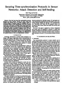
Fig. 1. Uncertainty time delay.
for and . Otherwise, the neighbor nodes may not successfully receive information from node within the time interval , which contradicts Assumption 2.1. The second key parameter is called relative skew, which is defined as follows. Definition 2.3: The relative skew is defined as (4)
where
is a constant and typically in the range of ( ) [38], [39]. It has been pointed out that and cannot be computed as the absolute reference time is not available to the sensor nodes [14], [35]. However, by comparing the local clock reading of one node with another local clock reading of node , we can obtain a relative clock between them, that is, It is known that the value of the hardware clock cannot be adjusted manually, because other hardware components may depend on a continuously running hardware clock in WSNs [15]. Hence, generally, a logical clock is applied to represent the synchronized time. Specifically, a logical clock value is a linear function of the hardware clock (3) where and are the logical clock skew and offset, respectively. Initially, it is common to set a constant for each node in advance so that each node broadcasts its message periodically with a period based on its own hardware clock. To simplify the statements and proofs later on, the data collisions are not taken into account in this paper. In fact, the data collision will not affect the convergence of our protocols. It turns out that under a common broadcast period , if all clocks are the same (or have the same skews and small offsets), collisions will occur constantly. One way to tackle this is by allowing communication asynchronously at random times, see, for instance, [11] and [16]. It should also be noted that there are many media-access control (MAC) protocols, for example, time-division multiple access (TDMA) and carrier-sense multiple access (CSMA), which can be easily incorporated for collision avoidance. The introduction of such a MAC protocol will not affect the main results of our paper. Moreover, Freris and Zouzias in [42] propose a randomized asynchronous approach which can be further adopted within each period to avoid the collision. Definition 2.2: Assume that every node broadcasts its message periodically with a common period based on its own hardware clock. is defined as the pseudoperiod [14]. For each node , its real period is given as . Since the clock skew is slightly different in general, the real period for . Under Assumption 2.1, we have
Since the skew compensation is always based on relative skew , the relative skew plays an important role in a synchronization protocol. The value of cannot be computed by (4) directly as and are unavailable, but it can be estimated with their hardware clock readings. The details will be given later on. C. Delay Model Communication delay has a direct impact on the accuracy of synchronization. Delays in packet delivery constitute a fundamental limitation in synchronizing clocks over WSNs [35]. In this paper, we will consider two cases as follows: 1) Delay Free: There is no transmission or reception delay. 2) Random Delay: The communication delays at different times are identically and independently distributed (i.i.d) positive random variables with constant mean and variance . Taking Fig. 1 as an example, node periodically broadcasts its hardware clock readings to its neighbor node , and node records its hardware clock readings as for , where and are the real broadcasting time and the receiving time for node and node , respectively. Thus, is the communication delay of the th communication from nodes to . Let for , where and denote the random delay of two consecutive communications, respectively. Then, it follows that the mean and variance of each random variable are equal to , respectively. Moreover, one infers that 0 and the random variables of each other for
and . Hence,
. Since are i.i.d, are also independent .
D. Problems of Interest The objective of time synchronization is to synchronize all of the nodes with respect to a common clock, given as (5) There always exists that for
for each logical clock .
such
HE et al.: TIME SYNCHRONIZATION IN WSNS
663
Our goal in this paper is to design a consensus-based clock for each node synchronization algorithm to find , such that (6) As pointed by [14], the real values of are not important; however, it is important that all clocks converge to one common virtual reference clock, and the final parameters only depend on the initial condition and the communication topology of the WSN. Remark 2.4: The linear clock model is widely used for time synchronization in WSNs, for example, [12]–[14] and [35]. Note that and may be slowly time varying in practice. However, as long as the synchronization algorithm can achieve certain accuracy in a short time, the algorithm can be restarted once the synchronization error exceeds a given bound. III. MTS PROTOCOL: DELAY-FREE CASE A. Maximum Time Synchronization (MTS) From (6), it is desirable to synchronize the clock skew and offset simultaneously. Since each hardware clock is a linear function of time and the communication delay between two connected nodes is omitted in the Delay Free case, each relative skew can be computed by (7) where and are two pair of hardware clock readings of nodes and with . In fact, when node receives time message from node , it reads its current hardware clock reading and stores ; meanwhile, when node receives the time message from node at the second time, the relative skew can be obtained from (7) based on these two pairs of historical records. We summarize the aforementioned process in the following algorithm (Maximum Time Synchronization). Algorithm 1 : Maximum Time Synchronization (MTS) 1:Given the initial conditions the common broadcast period
and to each node.
for
, set
If
, then
6:Store
.
In step 4, satisfies , which is the ratio of two nodes’ logical clock skew. Hence, node can know from whether its neighbor node has the larger logical clock skew. It follows from step 5 that for MTS, the logical clock skew and offset are adjusted simultaneously, and the fastest logical clock among neighbor nodes is selected as the reference clock. Remark 3.1: Since the protocol drives all nodes throughout the network to approach the maximum hardware clock, that is, maximum-consensus, we name the protocol as Maximum Time Synchronization. According to the protocol, the skew and offset compensations are conducted simultaneously and completed at the same time. Remark 3.2: For an arbitrary node , its hardware clock reading satisfies , where denotes the reality time at the th broadcast instant. Thus, we have for . B. Convergence of MTS Before proving the convergence of MTS, we first introduce . We use some preliminarily results. Define to denote the set of these nodes whose clock skews are equal to . Define . Let and , then the common clock (5) can be rewritten as (8) Let be the set of nodes whose logical clock skew and offset are equal to and at time , respectively. Clearly, the logical clock of nodes in are equivalent to the common clock described in (8). Since the initial condition and for in MTS, according to satisfies the definition of , it is clear that there exists at least one node whose hardware clock is equal to the common clock at the initial time, that is, . Let be the number of nodes belonging to the set at time . Define a function
, 2:If the current hardware clock reading of node satisfies , then node broadcasts its local hardware and to its neighbors. clock reading receives a packet from its neighbor node 3:If node time , then it records its local hardware clock reading and records the packet information as 4:If node has a historical record from according to (7) and by delete the record . 5:If
at
(9) Since
,
. Clearly, iff , which is equivalent to that if and only if . Theorem 3.3: Under Assumption 2.1 and using MTS, the skew and offset converge and satisfy for
.
, then compute . After that,
(10)
, then and . where Proof: The proof is given in Appendix A.
664
IEEE TRANSACTIONS ON AUTOMATIC CONTROL, VOL. 59, NO. 3, MARCH 2014
In order to simplify the statements, we make the following assumptions: Assumption 3.4: Assume that iff node receives messages more than once successfully from node within the time interval for all positive integers . Based on this assumption, node is defined to be neighboring with node in the time-interval iff node can receive messages more than once successfully from node within this interval. Theorem 3.5: Under Assumptions 2.1 and 3.4, the convergence time of MTS satisfies . Proof: From the proof of Theorem 3.3, we know that is a nonincreasing function. Assume at time (where ). Then, at each time interval , Assumption 2.1 ensures that there is at least an edge which connects one node and another node . Assumption 3.4 ensures that node can successfully receive messages from node at least twice within the time interval , which means that node can set its logical clock equal to the logical clock of node before . Hence, we have , that is, . Since , . It follows from the definition of that , then . Therefore, we have .
time-varying communication topology. Different from traditional time synchronization protocols, such as FTSP, MTS does not require setting a root node or building up a tree topology in advance, which largely reduces the implementing costs and enhances system robustness especially when the root node or nonleaf nodes are prone to various faults. Moreover, MTS can conduct both skew and offset compensation at the same time and complete them simultaneously in finite time. Note that different from the existing average consensus algorithms, the basic idea of our approach is to drive the logical clocks to the maximum value among all nodes so that the network can achieve time synchronization. In the algorithm, each node periodically broadcasts a packet containing its local hardware clock reading and its current relative logical clock and the offset , without requiring any feedback skew information from its neighbors. For each neighbor node , a pair of hardware clock readings needs to be stored by node . Compared with the recently developed consensus-based time synchronization algorithms, that is, GTSP [15] and ATS [14], the messages for MTS broadcast and storage are the same as these algorithms. Recently, Carli et al. in [28] and [29] proposed a promising average consensus-based time synchronization algorithm, where a distributed PI control law, based on the standard linear average consensus algorithm, is developed to achieve time synchronization. Although this algorithm achieves time synchronization asymptotically as in ATS and GTSP, it requires less computation and communication capabilities as each node has to keep in memory only two variables. During the communication, each node only transmits the value of its own logical clock while in the ATS, GTSP, and MTS algorithms, and each node has to keep in memory a number of variables which are proportional to the number of its neighbors. Comparing these average consensus-based time synchronization algorithms, the main advantage of MTS is its much faster convergence speed, that is, the average consensus-based time synchronization algorithms converge to global synchronization asymptotically, while MTS converges to global synchronization in a finite time. Energy cost is a major concern in WSNs. As the computational energy cost is comparably small due to the simple algorithm, we will focus on the communication energy cost, which can be measured by the broadcasting times. In the previous subsection, we have obtained an upper bound of the convergence time of MTS. Denote as the broadcasting times of node from the beginning to the time when the algorithm has just converged. Then based on Theorem 3.5, we obtain an upper bound of , given by
Remark 3.6: For Theorems 3.3 and 3.5, Assumption 2.1 is used to ensure that there are nodes in the set which can receive packets from the nodes in set . Clearly, we can replace it by the following assumption, which is commonly adopted in related works, for example, [17] and [35]. Assumption 3.7: An integer exists such that the graph is strongly connected for all non-negative integers . Remark 3.8: From the aforementioned theorems, MTS makes all nodes synchronize their logical clocks as the hardware clock of node with . Note that each satisfies (2) with , which means that each is approximately equal to 1, and all nodes’ logical clocks will be slightly faster or slower than the ideal time . If there is a misbehaving node with in the network, its neighbor node will observe from (7). Hence, node will easily know that node is an irregular node and isolate it. We can also set an upper bound, for example, , for each node , so that node will not utilize the information from its neighbor node if it detects . In this way, we can avoid the situation that the misbehaving node drives the clock speed much faster than the real time. Secure time synchronization under general malicious attacks, which is another interesting while challenging problem [40], [41], is beyond the scope of this paper, and will be pursued in our future research. C. Analysis of MTS Compared with the traditional tree-based or reference (root)-based time synchronization algorithms, for example, RBS [5], TPSN [6] and FTSP [7], etc., MTS has the advantage of being fully distributed, asynchronous, robust to packet drop, sensor node failure and new node joining, and it is adaptive to
(11) Assume that every broadcast of all nodes costs the same amount of energy and let be the total energy cost for MTS to convergence, then (12) From (12), it is not difficult to see that enlarging the common period can decrease the upper bound of . However, a larger will require a larger in order to ensure the connectivity, which
HE et al.: TIME SYNCHRONIZATION IN WSNS
665
may slow down the finite convergence time (seen from Theorem 3.5). Thus, it is a tradeoff between energy cost and convergence time. Obtaining an optimal is an interesting problem which depends on the real applications, and will be our future work. IV. WMTS PROTOCOL: RANDOM DELAY CASE There are also many cases when the communication delay between nodes is considerably large, which may severely affect the performance of time synchronization if ignored. Consider the random communication delay as modeled in Section II. Note that each relative skew , in MTS is computed based on two adjacent communications, i.e.,
A. Weighted Maximum Time Synchronization (WMTS) The accuracy of is crucial for time synchronizationl; thus, we will introduce a new method to estimate these relative skews. For , let . Assume that a node successfully obtains the messages from node at time , respectively. The following equation is used to estimate : (14) where . Equation (14) is an averaging process which is a classical stochastic approximation approach [37]. With the increase of , almost surely, which is the key to guarantee the convergence of WMTS. For , let , and let for . Since each satisfies , we have and
(13) where . Since is a random variable, is also a random variable. Thus, for each , it may be true that , which leads to . As a result, . This phenomenon will directly impact the accuracy of the synchronization and even make the logical clock diverge, as illustrated by the following example. 1) Example 4.1: Consider a network with two nodes indexed, respectively, by 1 and 2. According to MTS, if node 1 receives information times successfully from node 2 at time , then node 1 will update its logical clock based on . Since follows (13), that is, , . Then, from step 5 of we have for MTS, we have and for , that is, neither satisfies nor . Thus, node 1 is not able to fully synchronize its logical clock as node 2 since is random and with probability 0. Note that and , which means is nondecreasing and it will be updated to be equal to or larger than after node 1 receives information from node 2 at time . By a similar argument, for node 2, we also have as nondecreasing and it will be updated to be equal to or larger than after node 2 receives information from node 1 at time . Therefore, with the increasing communication between nodes 1 and 2, the logical clock skew of them increases continually with positive probability. Note that if the communication delay is equal to a constant, then we will have in (13), and then the entire network synchronization can still be guaranteed by MTS. Therefore, when the random delay in communication of the networks cannot be ignored, we need to revise the MTS algorithm accordingly so that time synchronization can still be achieved. In this section, we adopt the random delay model in Section II, and extend the MTS algorithm to handle the random communication delays.
Lemma 4.2: Assume that Then
(15) is obtained by (14). (16)
and (17) Proof: From (13), one notes that
Substituting the above equation into (14) yields
(18) Taking expectation on both sides of (18) yields (16). By computing the variance on both sides of (18), we have . Note that is the time interval between two consecutive instances when a node successfully receives messages from one neighbor node, hence . Therefore (19) for . Taking limitation on Clearly, both sides of (19) yields (17). In order to tackle the problems introduced by the communication delays, we adapt MTS to WMTS as follows. Algorithm 2 : Weighted Maximum Time Synchronization (WMTS) 1:Given the initial conditions , , and for . Set a common broadcast period to each node.
666
2:If including
IEEE TRANSACTIONS ON AUTOMATIC CONTROL, VOL. 59, NO. 3, MARCH 2014
,
,
, then node broadcasts packet and to its neighbors.
receives the packet -th time from node 3:If node at time , then record its local hardware clock reading and received clock information as and , respectively, for . , then compute 4:If compute .
according to (14), and then
5:If
and
or if
6:If where
and
, then compare and
and
, then
with
, . If
, then
7:Store
and
.
In WMTS, there are two decision variables and for each node , where denotes the source reference node of node , that is, node has updated its logical clock based on the estimate of the logical clock information of node , and represents the number of hops that the logical clock information of node is transmitted from the source reference node to node . Initially, we set the reference number and weight for , which means that node has not yet updated its logical clock by referring to any other nodes. During the iterations of WMTS, if two neighbor nodes and obtain different reference numbers, that is, , then the node with a larger logical clock will be selected as the reference node; if nodes and have the same reference number but different weight numbers, that is, , , then the node with a smaller weight number will be selected as the reference node. Meanwhile, after one node is selected as the reference node (assumed to be node ), node will adjust its decision variables and logical clock, such that , , and , while node will not update its decision variables and logical clock based on the messages received from node . Hence, with the use of decision variables and , two neighbor nodes with the same reference numbers cannot be the reference node to each other, and the phenomenon mentioned in Example 4.1 will not occur under WMTS. B. Convergence of WMTS Before proving the convergence of WMTS, we introduce a few preliminary results. Define , where and ( is the number of successful times that node receives information from node before time ) is a random and variable with (20)
Considering node with and at time , one can infer that node has obtained the logical clock information of node from a node which has and at time , and node has updated its parameters and based on the logical clock information of node obtained from node . Thus, we have and , where and is the number of times that node successfully receives messages from node within the time interval . Similarly, for node , one can infer that it has obtained the logical clock information of node from a node which has and at time . Therefore, given a time , for node with and , node sequence and time sequence exists with , such that the information is transmitted through the following path to node
where and , and each node receives information of node from node at time . Moreover, each node in the path finishes the last change of its logical clock within time based on the information of node obtained from node at time . Thus, for , we have and for , which means that these nodes have the same reference number but a different weight number. Hence, given a time , for each node with and , we can find a node path to transmit the logical clock information of reference node to node , where these nodes in the path have the same reference number and different weights. Note that the nodes in the path will be, in general, distinct. The reason is as follows. If there are two nodes (say and ) in , satisfying , which means that node has the same reference number but different weights at time and , we can infer the following two events: 1) Node has changed its reference number at a time , that is, . 2) There are nodes , in node sequence , where , which means there are at least two nodes which have obtained the logical clock information of node from node . ; thus, for , we have Note that for . Since the reference node satisfies for , it follows that holds for . Meanwhile, for WMTS, if two nodes and with different reference numbers contact each other at time , only when , node will change its reference number and update its logical clock skew such that , which increases the logical clock skew of node , that is, the logical clock skew of each node is increasing when it changes its reference number. Hence, for the first fact, one can infer that in expectation, and then as . However, the hardware clocks of nodes and are, in general, different from
HE et al.: TIME SYNCHRONIZATION IN WSNS
667
each other as . Thus, the first event will not occur in most cases. Furthermore, from WMTS, if two neighbor nodes and have the same reference number, then or holds, which means that the second event cannot occur in static networks or networks having only new nodes joining and nodes failure. Note that only when the aforementioned events occur simultaneously, there will be repeated nodes in node sequence . Therefore, without loss of generality, we assume that the nodes in node sequence are different from each other in the remainder of this paper. Let , and , and recall that is the random communication delay of two nodes at time , which follows a normal distribution. Theorem 4.3: Suppose that node has and at time . Then, for , there are node sequence and time sequence , such that (21) and
(22) are independent of where the random variables each other and is the number of successful times that node receives information from node before time . Proof: The proof is given in Appendix B. Theorem 4.3 provides the relationship of the logical clock between node and its reference node at time . Theorem 4.4: Under Assumptions 2.1 and 3.4, WMTS guarantees that (23) where clock satisfies
holds for , where a similar approach for offset estimation can asymptotically eradicate the offset error. In addition, the variance is crucial for synchronization accuracy. Since , it follows from (21) that:
Thus, for time
, from (23)
(25) where is the communication time from node to node within the time interval . From (25), it is clear that the variance of the error of each is a decreasing function on the variables . Thus, with more communication between nodes to , the variance of the error of each will decrease. Especially, if each variable in (25), the variance of the error of each converges to 0. However, Assumptions 2.1 and 3.4 do not guarantee that the upper bound provided in (25) is going to zero for . Thus, the WMTS algorithm does not guarantee that synchronization is reached completely. We will further discuss the detailed performance of WMTS in the simulation section. Although it is really difficult to obtain the analytical expression for the variance of each logical clock in the general timevariant network, we can rigorously prove that for the time-invariant network, WMTS converges in the mean square sense, which is given in the following Theorem. Theorem 4.5: Consider the time-invariant connected network. With WMTS, for , we have
and
. Moreover, the expected value of the logical (24)
. where Proof: The proof is given in Appendix C. Theorem 4.4 indicates that WMTS guarantees the finite-time convergence in expectation for time-variant networks. Note from the item in (24) that the synchronization error is affected by the weights of nodes and the expectation of random delay; thus, nodes with different weights will have slightly different expected logical clocks. This is the limitation caused by the random communication delay, as pointed out by Freris et al. [35], [36]. Meanwhile, when it takes two-way communication, the offset estimation methods proposed in [23] and [35] can be utilized to alleviate the offset error, for example, in the case where 0, the delay is known and equal to , from [35], the offset estimation is exact (just subtract the known delay in step 5 of WMTS); the same argument
Proof: The proof is given in Appendix D. With Theorem 4.5, it can be observed that under WMTS, the logical clock skew will converge asymptotically in the mean square sense in time-invariant connected networks. If the network is time variant, we can only guarantee that the expected value of each logical clock will converge in finite time, and the synchronization accuracy depends on the mean and the variance of the random delay. Although we cannot analytically provide the logical clock variance under time-variant networks, we conduct extensive large-scale network simulations which demonstrate that WMTS also provides good performance even for time-variant networks. Remark 4.6: Comparing WMTS and MTS, the basic idea is to drive the logical clocks to the maximum value among all nodes. Meanwhile, besides , , and , that is, hardware clock reading and two parameters of logical clock, which are needed in MTS, the broadcasting message of node in WMTS will additionally include and , that is, weight number
668
IEEE TRANSACTIONS ON AUTOMATIC CONTROL, VOL. 59, NO. 3, MARCH 2014
Fig. 3. Convergence time of MTS.
where and denote the maximum difference of the logical skew and of the logical offset between any two nodes, respectively. Clearly, the global time synchronization is reached iff and . A. Delay-Free Case
Fig. 2. Performance comparison in the static network. (a) MTS and ATS. (b) Skew and offset.
and reference number. In order to implement WMTS, each node will also need to store in addition to the hardware clock reading pair . The detailed performance comparison between MTS and WMTS will be provided in the simulation section. V. SIMULATION RESULTS For the simulation examples, we set and . Since the typical error for a quartz-crystal oscillator is [39], which corresponds to a 10 to 100 microsecond ( ), we assume that each skew of the hardware clock is randomly selected from the set , the offset of each node is randomly selected from the set . We also define two functions as follows:
(26)
We compare our algorithm MTS with ATS in [14]. Consider a static ring graph with 30. It is well recognized that distributed consensus-based algorithms often converge slowly for a ring graph. In Fig. 2(a), it can be observed that the skew synchronization is reached after 192 broadcasts (the total number of broadcast of all nodes) under MTS, while it takes more than 4000 broadcast to obtain comparable accuracy under ATS. In addition, from Fig. 2(b), it can be seen that for MTS, the skew and offset synchronization can be achieved simultaneously. Note that in MTS, each iteration denotes one broadcast of nodes. Based on 500 tests, the average iteration convergence time for MTS in this static network is 208, while it is more than 4145 to ensure ticks per second (where tick ) [14] under ATS. Fig. 3 shows how MTS converges with the number of sensors in the network, which shows the good scalability of MTS since the convergence time is almost linearly increasing with the number of sensors. Consider a dynamic graph with 50. The nodes are randomly deployed in an 100 100-m area at initial time 0, and the maximum communication range of each node is 20 m. Assume that each node may randomly change its position once every . As shown in Fig. 4(a), for by ATS; however, of MTS decreases to zero when the iteration time . Thus, the convergence speed of MTS is much faster than that of ATS in a dynamical network. Furthermore, Fig. 4(b) shows that and of MTS do converge to 0 at the same time 43 in the dynamical network. The average time for MTS is around 47, and is about 545 for ATS to ensure ticks per second.
HE et al.: TIME SYNCHRONIZATION IN WSNS
669
Fig. 5. Maximum skew among nodes changes under MTS and WMTS.
Fig. 4. Performance comparison in the dynamical network. (a) MTS and ATS. (b) Skew and offset.
B. Random Delay Case In the following simulations, we will consider the delay in the communication, and compare WMTS with MTS and ATS in [14]. Based on the empirical results in [7] and [34], without loss of generality, we assume that in the simulation, where is random positive communication delay, which means that the delay is in the range of with 99.97% confidence. Consider a static ring graph with 30. From Fig. 5, it can be observed that the maximum logical skew of nodes diverges under MTS, which confirms Example 4.1. However, under WMTS, it is clear that the maximum logical skew of nodes converges to a fixed constant. We also compare the performance of MTS, ATS, and WMTS under the static and dynamic network defined in the previous subsection, which are shown in Figs. 6 and 7, respectively. It is observed that WMTS always has faster convergence speed than that of ATS, and with better
Fig. 6. Compare the performance of MTS, ATS, and WMTS under the static network. (a) 0 to 4000. (b) 2000 to 4000.
synchronization accuracy than those of MTS and ATS. From Figs. 6(b) and 7(b), it is clear that WMTS has high accuracy
670
IEEE TRANSACTIONS ON AUTOMATIC CONTROL, VOL. 59, NO. 3, MARCH 2014
Fig. 7. Compare the performance of MTS, ATS, and WMTS under the dynamic network. (a) 0 to 1000. (b) 500 to 1000.
Fig. 8. Performance of WMTS with different mean and variance in the static network: (a) logical skew and (b) logical offset.
as the synchronization accuracy is less than 0.02 ticks/s (about 0.66 s/s) for the static and dynamic network. Next, we consider the relationship between synchronization error bound and the mean and variance of the random communication delay under WMTS. The error bound for skew compensation mainly depends on the variance but not on the mean of the delay, as the skew compensation depends on the estimate of relative skew [by (14)] which is only affected by the variance (seen from Lemma 4.2). However, it follows from (24) that the error bound for the offset compensation is mainly affected by the mean . As shown in Fig. 8, the error bound will increase with the variance for skew compensation [see Fig. 8(a)] while with mean for offset compensation [see Fig. 8(b)]. Fortunately, for skew compensation, it follows from Fig. 8(a) that the error bounds are always less than 0.3 ticks/s (about 10 s/s) for (which means that there is a delay in the range of with 99.97% confidence), that is, WMTS guarantees that the error bound is less than 10 s even if the communication delay is in the order of microseconds. Note that
skew compensation is more important since it can extend the re-synchronization period to save energy; thus, WMTS is able to well handle the random delay case. Especially, if (the delay in with a 99.97% confidence), WMTS will guarantee that the error bounds for skew compensation and offset compensation will be less than s and 5 s, respectively, which means that with WMTS, the maximum logical clock difference between nodes will be less than 10 s in the time interval s after convergence of the algorithm. Finally, the performance of WMTS with different means and variances in a dynamic network is shown as in Fig. 9, where the relationship between synchronization error bound and the values of mean and variance are the same as those in the static network. Moreover, by comparing Figs. 9 with 8, it is observed that for both skew and offset compensation, the synchronization accuracy of WMTS in the dynamic network is improved with even faster converging speed. The reason is that the random dynamic network may help to improve network connectivity which accelerates the consensus process.
HE et al.: TIME SYNCHRONIZATION IN WSNS
671
logical clocks are equal to and accordingly. Hence, it suffices to prove 0. We first prove that is nonincreasing. For any arbitrary , its skew and offset node are equal to and , respectively. Hence, holds for , which means holds for . In other words, this node will not update its logical clock skew any more as for . Furthermore, ensures that node has the largest logical clock offset from the definition of , which is equivalent to . Therefore, each node in will keep its logical clock skew and offset, which means that is nondecreasing which, in turn, implies that is nonincreasing. Assume at time (where ). Then, there is at least one node in the network which is not in the set . Assumption 2.1 guarantees that the network is connected during any time interval , which means that there are edge sequences which connect nodes ( ) and ( ). Hence, exists such that node in receives packets from node in at time for the second time by two communication links existing between nodes and , where the two edges are in . According to MTS, node will update its logical clock and then nodes and will have the same logical clock, which means that node belongs to . Thus, , that is, satisfies . Hence, will decrease strictly if . Notice that is finite; therefore, . APPENDIX B PROOF OF THEOREM 4.3
Fig. 9. Performance of WMTS with different mean and variance in the dynamic network: (a) logical skew and (b) logical offset.
VI. CONCLUSION We investigate the time synchronization for WSNs in this paper. We present two new time synchronization algorithms— MTS and WMTS protocols for WSNs with delay free and random delay cases, respectively. These two algorithms conduct the skew and offset compensations simultaneously. The main idea is to drive all clocks to the maximum value among the network. It is proved that the MTS algorithm converges within a finite time and the expected convergence time of WMTS is also finite. Both algorithms are fully distributed, asynchronous, and robust to dynamic network topologies. Extensive simulations demonstrate the effectiveness of the proposed algorithms. Future directions include extending the idea to more complicated network models and experimental validation of the results. APPENDIX A PROOF OF THEOREM 3.3 Proof: According to the definitions of in (8) and in (9), it is obvious that once 0, the skew and offset of all
0 and Proof: For WMTS, if node has at time , the reference node of node is itself, then node has not adjusted its logical clock, that is, and . If node has and at time , node makes the latest change of its logical clock, reference number, and weight when it communicates with a node which has and at an earlier time . Thus, we have (27) and are equal to the number of successful where times that node received information from node within , and
(28) is the random communication delay from node to where node of the communication at time . For node , similar to the previous discussion, one can obtain (29)
672
IEEE TRANSACTIONS ON AUTOMATIC CONTROL, VOL. 59, NO. 3, MARCH 2014
where and successful times that node within , and
are equal to the number of receives information from node
and with (35) yields
and
. Combining (34) (36)
(30) and , and where node has . Substituting (29) and (30) into (27) and (28), respectively, yields (31) and
and (37) From the above inequalities and using Theorem 4.3, one can conclude that (33) holds. Case 2: The reference numbers of them are updated as . The remaining discussion is similar to that of Case 1. Case 3: The reference numbers of them are updated as and . In this case, and during the communication between nodes and . Hence (38)
(32) . By repeating this procedure, until the where weight of a node is equal to 0, one obtains (21) and (22) and the node sequence. Since the nodes in such a node sequence are different, the random variables in (21) and (22) are independent of each other. APPENDIX C PROOF OF THEOREM 4.4 be series random variables Let to denote which are independent of each other. Use that and . Lemma C.1: Suppose that two neighbor nodes and have two successful communications within the time interval . By WMTS, we have
(33) where is the finishing time of the two successful communications. Proof: If , (33) is obtained directly from step 5 and Theorem 4.3. If , from steps 5 and 6 of the WMTS algorithm, three cases may appear for nodes and after two successful communications between them. Case 1: The reference numbers of them are updated as . In this case, nodes to
, where is the communication times from within . Hence
With WMTS,
and
satisfy (39)
and and . Thus, with (38) and (39) and Theorem 4.3, the Lemma holds. Taking expectation on both sides of (33), we have , that is, after two successful communications between two nodes, the node with faster hardware clock speed will be selected as the source reference clock. Lemma C.2: Under Assumptions 2.1 and 3.4, WMTS guarantees that (40) where . Proof: Divide the time interval into small time intervals, which are given by , , , . According to Assumption 2.1, the network is connected at each small time interval. Assume that node with its hardware clock is equal to (8), that is, . Since the network is connected within each small time interval, there is at least one node, say , which will be a neighbor of node within . Assumption 3.4 ensures that node and have at least two successful communications within . After two communications, from Lemma C.1
(41) where is the finishing time of two successful communications between them. Note that . Combining (41) with Theorem 4.3 yields that
(34) With WMTS,
and
satisfy (35)
(42) where is the number of nodes in set satisfying
which is the node .
HE et al.: TIME SYNCHRONIZATION IN WSNS
673
In the time interval , the network is also connected, and there is at least one node, say , in the network, which will be a neighbor node of or (assume it is node here). From Lemma 1.1, after two successful communications between nodes and
Combining (47) and (46) with Theorem 4.3 gives
(49) where
is the number of nodes in
which satisfies
(43) is the finishing time of two successful where communications between them. We have . Note that node may contact with only within , that is, . Hence
From the aforementioned discussion, one concludes that (48) and (49) hold for . It follows that all nodes belong to and satisfy (49). Since , we have
Combining (43) and (42) with Theorem 4.3, one can obtain Therefore, we obtain (44) where
is the number of nodes in
which is defined as .
(50)
By induction, assume that (45) and
(46) holds for in
, where which satisfies
is the number of nodes
Taking expectation on both sides of (50) yields . At the same time, note that holds for . Thus, (40) holds. From Lemma C.2, the expected value of the reference node is equal to that of the node whose hardware clock skew is . Note that the clock oscillators for sensor nodes are slightly different, which means that the hardware clock skew of nodes is also slightly different. Hence, by combining Lemma 1.2 and Theorem 4.3, we can obtain Theorem 4.4. APPENDIX D PROOF OF THEOREM 4.5
Then, within , there is a node , which becomes a neighbor node of one node in (assume it is ). Similarly, from Lemma 1.1
each
Proof: Since the network is time-invariant and connected, of the random variable in Theorem 4.3 satisfies when . From (20) (51)
Hence, from Theorem 4.3, we have (47) is the finishing time of two sucwhere cessful communications between and . We have . Note that nodes may contact with only in , which guarantees that
From (45), we have (48)
and (52) Furthermore, for any neighboring nodes and , from Lemma 1.1, . Since the network is connected, it follows that (52) holds for . Therefore, for , it follows from (52) that and
674
IEEE TRANSACTIONS ON AUTOMATIC CONTROL, VOL. 59, NO. 3, MARCH 2014
REFERENCES [1] J. He, P. Cheng, L. Shi, and J. Chen, “Time synchronization in WSNs: A maximum value based consensus approach,” in Proc. CDC, Dec. 12–15, 2011, pp. 7882–7887. [2] B. Sundararaman, U. Buy, and A. D. Kshemkalyani, “Clock synchronization for wireless sensor networks: A survey,” Ad Hoc Netw., vol. 3, no. 3, pp. 281–323, 2005. [3] J. Du and W. Shi, “APP-MAC: An application-aware event-oriented MAC protocol for multimodality wireless sensor networks,” IEEE Trans. Vehicular Technol., vol. 57, no. 6, pp. 3723–3731, Nov. 2008. [4] Q. Li and D. Rus, “Global clock synchronization in sensor networks,” presented at the Infocom, Hong Kong, China, Mar. 2004. [5] J. Elson, L. Girod, and D. Estrin, “Fine-grained network time synchronization using reference broadcasts,” presented at the Operating Syst. Design Implement., Boston, MA, USA, Dec. 9–11, 2002. [6] S. Ganeriwal, R. Kumar, and M. B. Srivastava, “Timing-sync protocol for sensor networks,” in Proc.SenSys, 2003, pp. 138–149. [7] M. Maroti, B. Kusy, G. Simon, and A. Ledeczi, “The flooding time synchronization protocol,” in Proc. ACM SenSys, 2004, pp. 39–49. [8] Y. R. Faizulkhakov, “Time synchronization methods for wireless sensor networks: A survey,” Programm. Comput. Softw., vol. 33, no. 4, pp. 214–226, 2007. [9] R. Solis, V. S. Borkar, and P. R. Kumar, “A new distributed time synchronization protocol for multihop wireless networks,” in Proc. IEEE CDC, San Diego, CA, USA, Dec. 2006, pp. 2734–2739. [10] A. Giridhar and P. R. Kumar, “Distributed clock synchronization over wireless networks: Algorithms and analysis,” in Proc. IEEE CDC, 2006, pp. 4915–4920. [11] M. Akar and R. Shorten, “Distributed probabilistic synchronization algorithm for communication networks,” IEEE Trans. Autom. Control, vol. 53, no. 1, pp. 389–394, Feb. 2008. [12] N. Marechal, J. Pierrot, and J. Gorce, “Fine synchronization for wireless sensor networks using gossip averaging algorithms,” in Proc. IEEE ICC, 2008, pp. 4963–4967. [13] C. Liao and P. Barooah, “Time-synchronization in mobile sensor networks from difference measurements,” in Proc. CDC, 2010, pp. 2118–2123. [14] L. Schenato and F. Fiorentin, “Average TimeSynch: A consensus-based protocol for time synchronization in wireless sensor networks,” Automatica, vol. 47, no. 9, pp. 1878–1886, 2011. [15] S. Philipp and W. Roger, “Gradient clock synchronization in wireless sensor networks,” in Proc. IPSN, 2009, pp. 37–48. [16] R. Olfati-Saber, J. A. Fax, and R. M. Murray, “Consensus and cooperation in networked multi-agent systems,” Proc. IEEE, vol. 95, no. 1, pp. 215–233, Jan. 2007. [17] A. Nedic, A. Olshevsky, A. Ozdaglar, and J. N. Tsitsiklis, “On distributed averaging algorithms and quantization effects,” IEEE Trans. Autom. Control, vol. 54, no. 11, pp. 2506–2517, Nov. 2009. [18] S. Boyd, A. Ghosh, B. Prabhakar, and D. Shah, “Randomized gossip algorithms,” IEEE Trans. Inf. Theory, vol. 52, no. 6, pp. 2508–2530, Jun. 2006. [19] G. Xiong and S. Kishore, “Analysis of distributed consensus time synchronization with Gaussian delay over wireless sensor networks,” EURASIP J. Wireless Commun. Netw., 2009. [20] Q. Chaudhari, E. Serpedin, and K. Qaraqe, “Some improved and generalized estimation schemes for clock synchronization of listening nodes in wireless sensor networks,” IEEE Trans. Commun., vol. 58, no. 1, pp. 63–67, Jan. 2010. [21] J. Elson, R. M. Karp, C. H. Papadimitriou, and S. Shenker, “Global synchronization in sensornets,” in Proc. Latin Amer. Symp., 2004, pp. 609–624. [22] P. Barooah and J. P. Hespanha, “Distributed estimation from relative measurements in sensor networks,” in Proc. ICISIP, 2005, pp. 226–231. [23] N. M. Freris, V. S. Borkar, and P. R. Kumar, “A model-based approach to clock synchronization,” in Proc. CDC, 2009, pp. 5744–5749. [24] D. Fontanelli and D. Macii, “Towards master-less WSN clock synchronization with a light communication protocol,” in Proc. IMTC, 2010, pp. 105–110. [25] L. Mei and Y. C. Wu, “On clock synchronization algorithms for wireless sensor networks under unknown delay,” IEEE Trans. Veh. Technol., vol. 59, no. 1, pp. 182–190, Jan. 2010.
[26] L. Mei and Y.-C. Wu, “Distributed clock synchronization for wireless sensor networks using belief propagation,” IEEE Trans. Signal Process., vol. 59, no. 11, pp. 5404–5414, Nov. 2011. [27] R. Carli, A. Chiuso, S. Zampieri, and L. Schenato, “A PI consensus controller for networked clocks synchronization,” in Proc. 17th IFAC World Congr., 2008, pp. 10289–10294. [28] R. Carli and S. Zampieri, “Networked clock synchronization based on second order linear consensus algorithms,” in Proc. CDC, 2010, pp. 7259–7264. [29] R. Carli, E. Elia, and S. Zampieri, “A PI controller based on asymmetric gossip communications for clocks synchronization in wireless sensors networks,” in Proc. CDC-ECC, 2011, pp. 7512–7517. [30] R. Carli, A. Chiuso, L. Schenato, and S. Zampieri, “Optimal synchronization for networks of noisy double integrators,” IEEE Trans. Autom. Control, vol. 56, no. 5, pp. 1146–1152, May 2011. [31] W. Ren, “On consensus algorithms for double-integrator dynamics,” IEEE Trans. Autom. Control, vol. 53, no. 6, pp. 1503–1509, Jul. 2008. [32] R. Olfati-Saber and R. M. Murray, “Consensus protocols for networks of dynamic agents,” in Proc. ACC, 2003, pp. 951–956. [33] H. Tijms, Understanding Probability: Chance Rules in Everyday Life. Cambridge, U.K.: Cambridge Univ. Press, 2004. [34] Z. Zhong, P. P. Chen, and T. He, “On-demand time synchronization with predictable accuracy,” in Proc. IEEE Infocom, 2009, pp. 2480–2488. [35] N. M. Freris, S. R. Graham, and P. R. Kumar, “Fundamental limits on synchronizing clocks over networks,” IEEE Trans. Autom. Control, vol. 56, no. 6, pp. 1352–1364, Jun. 2011. [36] N. M. Freris, H. Kowshik, and P. R. Kumar, “Fundamentals of large sensor networks: Connectivity, capacity, clocks, and computation,” Proc. IEEE, vol. 98, no. 11, pp. 1828–1846, Nov. 2010. [37] J. R. Birge and F. Louveaux, Introduction to Stochastic Programming. New York, USA: Springer, 1997. [38] D. Zhou and T. H. Lai, “An accurate and scalable clock synchronization protocol for IEEE 802.11-based multihop Ad Hoc networks,” IEEE Trans. Parallel Distrib. Syst., vol. 18, no. 12, pp. 1797–1808, Dec. 2007. [39] B. Choi, H. Liang, X. Shen, and W. Zhuang, “DCS: Distributed asynchronous clock synchronization in delay tolerant networks,” IEEE Trans. Parallel Distrib. Syst., vol. 23, no. 3, pp. 491–504, Mar. 2012. [40] S. Ganeriwal, C. Popper, S. Capkun, and M. B. Srivastava, “Secure time synchronization in sensor networks,” ACM Trans. Inf. Syst. Security, vol. 11, no. 4, 2008. [41] J. Chiang, J. Haas, Y.-C. Hu, P. R. Kumar, and J. Choi, “Fundamental limits on secure clock synchronization and man-in-the-middle detection in fixed wireless networks,” in Proc. Infocom, 2009, pp. 1962–1970. [42] N. M. Freris and A. Zouzias, “Fast distributed smoothing of relative measurements,” in Proc. CDC, 2012, pp. 1411–1416.
Jianping He is currently pursuing the Ph.D. degree in control science and engineering at Zhejiang University, Hangzhou, China. His research interests include time synchronization, consensus, and distributed security algorithm design problems in wireless sensor networks. Dr. He is a member of the Group of Networked Sensing and Control (IIPC-nesC), State Key Laboratory of Industrial Control Technology, Zhejiang University.
Peng Cheng (M’10) received the B.E. degree in automation and the Ph.D. degree in control science and engineering from Zhejiang University, Hangzhou, China, in 2004 and 2009, respectively. Currently, he is Associate Professor with the Department of Control Science and Engineering, Zhejiang University. His research interests include networked sensing and control, cyberphysical systems, and robust control. Dr. Cheng serves as the publicity Co-Chair for IEEE MASS 2013.
HE et al.: TIME SYNCHRONIZATION IN WSNS
Ling Shi received the B.S. degree in electrical and electronic engineering from the Hong Kong University of Science and Technology, Hong Kong, China, in 2002 and the Ph.D. degree in control and dynamical systems from the California Institute of Technology, Pasadena, CA, USA, in 2008. Currently, he is an Assistant Professor at the Department of Electronic and Computer Engineering, Hong Kong University of Science and Technology. His research interests include networked control systems, wireless sensor networks,
675
QoS and Reliability Symposium Co-Chair, IEEE SmartGridComm The Whole Picture Symposium Co-Chair, IEEE MASS 2013 Local Chair, Wireless Networking and Applications Symposium Co-Chair, IEEE ICCC 2013 and TPC member for IEEE ICDCS’10,’12,’13; IEEE MASS’10,’11,’13; IEEE SECON’11,’12; IEEE INFOCOM’11,’12,’13, etc. He is currently Associate Editors for several international journals, including IEEE TRANSACTIONS ON PARALLEL AND DISTRIBUTED SYSTEMS, IEEE TRANSACTIONS ON INDUSTRIAL ELECTRONICS, IEEE Network, IET Communications, etc. He was a guest editor of IEEE TRANSACTIONS ON AUTOMATIC CONTROL, Computer Communication, Wireless Communication and Mobile Computer, and Journal of Network and Computer Applications.
and distributed control.
Jiming Chen (M’08–SM’11) received the B.Sc. and Ph.D. degrees in control science and engineering from Zhejiang University, Hangzhou, China, in 2000 and 2005, respectively. He was a Visiting Researcher at INRIA in 2006, National University of Singapore in 2007, and the University of Waterloo, Waterloo, ON, Canada, from 2008 to 2010. Currently, he is a Full Professor with the Department of Control Science and Engineering, and the coordinator of group of Networked Sensing and Control in the State Key Laboratory of Industrial Control Technology, and Vice Director of the Institute of Industrial Process Control at Zhejiang University, Hangzhou, China. Dr. Chen also served/serves as Ad hoc and Sensor Network Symposium Co-Chair, IEEE Globecom 2011; General Symposia Co-Chair of ACM IWCMC 2009 and ACM IWCMC 2010, WiCON 2010 MAC track Co-Chair, IEEE MASS 2011 Publicity Co-Chair, IEEE DCOSS 2011 Publicity Co-Chair, IEEE ICDCS 2012 Publicity Co-Chair, IEEE ICCC 2012 Communications
Youxian Sun joined the Department of Chemical Engineering, Zhejiang University, Hangzhou, China, in 1964. From 1984 to 1987, he was an Alexander Von Humboldt Research Fellow and Visiting Associate Professor at the University of Stuttgart, Stuttgart, Germany. He has been a Full Professor at Zhejiang University since 1988. In 1995, he was elevated to an Academician of the Chinese Academy of Engineering, China. He is author/co-author of 450 journal and conference papers. Currently, he is the Director of the Institute of Industrial Process Control and the National Engineering Research Center of Industrial Automation, Zhejiang University. His current research interests include modeling, control, and optimization of complex systems, and robust control design and its applications. Prof. Sun is President of the Chinese Association of Automation. He also served as Vice-Chairman of IFAC Pulp and Paper Committee and Vice-President of the China Instrument and Control Society.