timed continuous Petri nets, since they are relevant for boundedness and liveness. In particular, it is studied the connection between these properties and the net ...
Timing-dependent boundedness and liveness in continuous Petri nets ⋆ C. Renato V´ azquez ∗ Manuel Silva ∗ ∗
Dep. de Inform´ atica e Ingenier´ıa de Sistemas, Centro Polit´ecnico Superior, Universidad de Zaragoza, Mar´ıa de Luna 1, E-50018 Zaragoza, Spain (e-mail: {cvazquez,silva}@unizar.es) Abstract: The very classical structural boundedness and repetitiveness properties for discrete and untimed models are reconsidered for timed continuous Petri nets (T CP N ), under infinite server semantics. The timing is here involved in the analysis, by taking advantage of its matricial characterization and properties analogous to conservativeness and consistency are defined. It is shown that such properties are sufficient for timed boundedness and timed liveness, respectively, even if the untimed model does not exhibit them. The rest of the paper is devoted to study these timing-dependent boundedness and liveness. Keywords: Petri-nets; Continuous Systems; Safety analysis; Concurrent systems. 1. INTRODUCTION An impressive amount of results related to the analysis of qualitative properties of discrete event systems (DES) can be found in the literature. Applications involve a wide range of systems including manufacturing process, telecommunication, traffic and logistic systems. Unfortunately, for large models, the analysis based on enumerative techniques becomes prohibitive, since the number of states increases exponentially. For this reason, the fluidification has been proposed as a relaxation in which discrete event systems are studied through continuous approximated models, reducing thus the computational complexity involved in the analysis and synthesis problems. Furthermore, by using fluid models, more analytical techniques can be used for the analysis of some interesting properties. In Petri nets (PN), fluidification has been introduced from different perspectives (David & Alla (2005), Silva & Recalde (2004), Balduzzi, Menga & Giua (2000)). In this work, timed continuous Petri net (TCPN) models under infinite server semantics (ISS) are considered, since it has been found that such systems best approximate interesting classes of DES. An interesting approach, when qualitative properties of discrete Petri nets are analyzed, is the so called structural theory. According to this, important information about the behavior of the system is obtained from the structure of the net, considering the initial marking as a parameter. For general models, structural techniques give conditions, usually in one way (sufficient or necessary), for the properties under study. Obviously, if the analysis is restricted to particular subclasses, stronger results can ⋆ This work was partially supported by project CICYT and FEDER DPI2006-15390. The research leading to these results has received funding from the European Community’s Seventh Framework Programme (FP7/20072013) under grant agreement no 224498.
be obtained. In the literature, a lot of results related to the computation of structural components can be found (e.g., Silva, Teruel & Colom (1998), Huck, Freiheit & Zimmermann (2000)). Components that are important for the system’s behavior are traps, siphons and (semi)flows. In some cases, these allow the verification of behavioral properties, like boundedness and liveness (see, for instance, Silva, Teruel & Colom (1998), David & Alla (2005)). In this way, it seems interesting to extend the structural analysis to fluid Petri nets, in order to obtain information about its behavior. From this approach, Recalde, Teruel & Silva (1999) provided results for the autonomous model obtained from structural analysis. J´ ulvez, Recalde & Silva (2006) advanced this kind of studies for the timed continuous system (under ISS). Since the integrality constraints are removed in the continuous nets, structural properties have a stronger meaning. Moreover, regarding T CP N ’s, timing rates can be also considered with the structural analysis, since it is characterized in a matricial form (Λ). Among the different str. properties, in this work str. boundedness and str. repetitiveness will be analyzed for timed continuous Petri nets, since they are relevant for boundedness and liveness. In particular, it is studied the connection between these properties and the net structure and timing. After briefly introducing basic definitions and notation (section 2), general ideas about str. boundedness and str. repetitiveness are recalled in section 3. In section 4, analogous properties to conservativenes and consistency are defined for T CP N systems, in which the timing is also considered. Since these properties are related to boundedness and liveness, the existence of these is studied, first for general nets (section 5), later for particular subclasses of nets and siphons (section 6). Finally, in section 7 those results are used in order to enforce timed-liveness and boundedness through the timing, when the untimed model does not exhibit such properties.
2. BASIC CONCEPTS We assume that the reader is familiar with Petri nets. The set of the input (output) nodes of v is denoted as • v (v • ). The structure N = hP, T, Pre, Posti of continuous Petri nets (ContP N ) is the same as the structure of discrete P N s. That is, P is a finite set of places, T is a finite set of transitions with P ∩ T = ∅, Pre and Post are |P | × |T | sized, natural valued, pre- and post- incidence matrices. We assume that N is connected and that every place has a successor, i.e., |p• | ≥ 1. The usual P N system, hN , M0 i, will be said to be discrete so as to distinguish |P | it from a continuous P N system, in which m ∈ R≥0 . The main difference between both formalisms is in the evolution rule, since in ContP N s firing is not restricted to be done in integer amounts (David & Alla (2005), Silva & Recalde (2004)). As a consequence the marking is not forced to be integer. A transition t is enabled at m iff for every p ∈ • t, m(p) > 0, and its enabling degree is enab(t, m) = minp∈• t {m(p)/Pre(p, t)}. The firing of t in a certain amount α ≤ enab(t, m) leads to a new marking m′ = m+α·C(t), where C = Post−Pre is the token-flow matrix and C(t) represents the t − th column of C, which is related to transition t. In the sequel, given a matrix (vector) A, [A]j denotes the j-th column (entry) of A. As in discrete systems, a column vector y s.t. yT · C = 0 (x s.t. C · x = 0) is called P-flow (T-flow ). When they are nonnegative, they are called P- and T-semiflows. Here, we always consider net systems whose m0 marks all P-semiflows (otherwise, all the transitions in the Pcomponent will be non-live). Matrix By denotes a basis of P − f lows. If there exists y > 0 s.t. yT · C = 0 (yT · C ≤ 0), the net is said to be conservative Cv (structurally bounded ), and if there exists x > 0 s.t. C · x = 0 (C · x ≥ 0) the net is said to be consistent Ct (structurally repetitive). A set of places Σ is a siphon iff • Σ ⊆ Σ• (the set of input transitions is included in the corresponding output one), and it is minimal if it does not contain another siphon. A net is strongly connected (P-strongly connected ) iff for every pair of nodes (places) x and y, there is a path leading from x to y. Two transitions t and t′ are said to be in conflict if • t ∩• t′ 6= ∅. A conflict {t, t′ } is said to be topologically equal (equivalently, t and t′ are in topological equal conflict relation) if ∃γ > 0 s.t. P re[P, t] = γP re[P, t′ ]. Subclasses of nets are defined according to their structure: 1) N is Conflict-free (CF) iff ∀p ∈ P : |p• | ≤ 1. 2) N is Join-free (JF) iff ∀p ∈ T : |• t| ≤ 1. 3) N is Fork-Attribution (FA) iff it is CF and JF. 4) N is Topologically Equal Conflict (TEC) iff all the conflicts are topologically equal. A Timed Continuous Petri Net (T CP N ) is a continuous |T | P N together with a vector λ ∈ R>0 . There are two main semantics defined for continuous timed transitions: infinite server (ISS) or variable speed, and finite server (FSS) or constant speed (see Silva & Recalde (2004),David & Alla (2005)). Here, ISS will be considered, since it usually provides a better approximation to the original model. Under ISS, the flow through a timed transition t is the product of the rate, λ(t), and enab(t, m), the instantaneous enabling degree of the transition, i.e., f (t, m) = λ(t)·
enab(t, m) = λ(t) · minp∈• t {m(p)/Pre(p, t)}. For the flow to be well defined, every transition must have at least one input place. The “min” in the above definition leads to the concept of configurations: a configuration assigns to each transition one input place that for some markings will control (constraint) its firing speed. Q An •upper bound for the number of configurations is t∈T | t|. The set of all nonnegative markings that agree with the P-flows is denoted as Class(m0 ), so, any reachable marking belongs to it. This set plays the role of a “state space” in T CP N systems, and it can be divided into marking regions, denoted by ℜ, according to the configurations. These regions are polyhedrons, and are disjoint, except on the borders. The flow through the transitions can be written as f (m) = ΛΠ(m)m, where Λ is a diagonal matrix whose elements are those of λ, and Π(m) is the configuration operator matrix at m, which is defined by elements as 1 if pj is constraining ti Π(m)i,j = Pre(pj , ti ) 0 otherwise
If more than one place is constraining the flow of a transition at a given marking, any of them can be used, but only one is taken. Thus, each region ℜi is associated to a valuation for the configuration matrix Πi . Notice that the i-th entry of the vector Π(m)m is equal to the enabling degree of transition ti . The dynamical behavior of a T CP N system is described by its state equation: •
m = CΛΠ(m)m
(1)
Recalde, Teruel & Silva (1999) introduced the concept of lim-liveness and structural lim-liveness for autonomous continuous Petri nets: an autonomous model hN , m0 i is lim-live iff for every transition tj and for any marking m reachable from m0 (allowing infinite sequence of firings), a successor m′ exists such that enab(tj , m′ ) > 0. A net N is structurally lim-live iff ∃m0 such that hN , m0 i is lim-live. Those concepts were extended by J´ ulvez, Recalde & Silva (2006) to T CP N ’s: assuming that exists a steady state, a T CP N system hN , λ, m0 i is timed-live if the flow vector at the steady state is fss > 0. Similarly, a timed-net hN , λi is structural timed-live iff there exists an initial marking m0 such that the system hN , λ, m0 i is timed-live. 3. STRUCTURAL BOUNDEDNESS AND REPETITIVENESS IN UNTIMED PETRI NETS: DISCRETE VS CONTINUOUS Some classic results related to boundedness, repetitiveness and liveness in untimed discrete and continuous Petri net models are here recalled. As expected, by structural analysis stronger results can be obtained for continuous models . The study of boundedness and repetitiveness in discrete Petri nets includes very well known results based on structural analysis. For instance, recalling from Silva, Teruel & Colom (1998), given a P/T net N , the following three statements are equivalent:
1) N is structurally bounded, i.e., every place is bounded for every M0 . 2) There exists y > 0 s.t. yT C ≤ 0. 3) There does not exist x ≥ 0 s.t. Cx 0.
be obtained from an algebraic approach. First, a necessary condition for reachability inside a region is obtained: If m′ ≥ 0 is reachable trough a trajectory inside ℜi , then there exists σ ≥ 0 s.t. m′ = m0 + CΛΠi σ.
Structural boundedness is sufficient but not necessary for boundedness. The necessary condition is not obtained in general, since reachability (in discrete Petri nets) cannot be fully characterized in an algebraic way. Actually, previous results were obtained by characterizing str. boundedness with the following necessary reachability condition: if M′ is reachable then M′ ≥ 0 and ∃σ ≥ 0 s.t. M′ = M + Cσ.
This condition is trivially obtained by integrating the state Rτ equation (1), thus: m(τ ) = m0 + CΛΠi 0 m(η)dη, where Rτ Rτ m(η)dη ≥ 0, and substituting 0 m(η)dη = σ. Notice 0 that this necessary reachability condition is similar to that of discrete nets (but in this CΛΠi appears instead of C). Then, by proceeding in a similar way to the structural analysis for discrete nets, the following analogous results are obtained: Proposition 1. Given a T CP N system, while it evolves inside region ℜi , the following three statements are equivalent: I.1) The system behaves as structurally bounded, i.e., every place is bounded for every m0 ∈ ℜi . I.2) There exists w > 0 s.t. wT CΛΠi ≤ 0. I.3) There does not exist v ≥ 0 s.t. CΛΠi v 0. Similarly, while the system evolves inside region ℜi the following three statements are equivalent: II.1) The system behaves as structurally repetitive, i.e., every transition is repetitive for some m0 ∈ ℜi . II.2) There does not exist w > 0 s.t. wT CΛΠi 0. II.3) There exists v > 0 s.t. CΛΠi v ≥ 0.
Those results are also valid for continuous Petri net models. Furthermore, if all the transitions are fireable from m0 (i.e., there exist no empty siphon), then str. boundedness is not only sufficient, but also necessary for boundedness in the continuous net (Recalde, Teruel & Silva (1999)): if all the transitions are fireable from m0 , then m′ is reachable iff ∃σ ≥ 0 s.t. m′ = m + Cσ ≥ 0, i.e., the necessary condition for reachability used in the structural analysis of discrete nets becomes also sufficient for the continuous model. The dual concept of boundedness is repetitiveness. Regarding to this property, the following result, which was obtained by using the same necessary condition for reachability, is recalled from (Silva, Teruel & Colom (1998)): Given a P/T net N , the following three statements are equivalent: 1) N is structurally repetitive, i.e., every transition is repetitive for some M0 . 2) There does not exist y > 0 s.t. yT C 0. 3) There exists x > 0 s.t. Cx ≥ 0. These results are also valid for the continuous net. Furthermore, if all the transitions are fireable from m0 then, by following a similar reasoning as in the previous case, it can be proved that str. repetitiveness becomes not only necessary but also sufficient for repetitiveness in the continuous model. Finally, it is known that a continuous P N system fall into non-liveness iff a marking, in which a siphon is empty, is reached. Therefore, given a continuous P N system in which the initial marking is positive m0 > 0 (thus all transitions are fireable), the system is non-live iff there exists a siphon Σ and ∃mf , σ ≥ 0 s.t. mf = m0 + Cσ and ∀p ∈ Σ, mf (p) = 0. Obtaining thus a necessary and sufficient condition for liveness based on structural components. This condition is necessary for non-liveness in the general case (i.e., m0 ≯ 0), as proved in (Recalde, Teruel & Silva (1999), theorem 9). 4. TIMING-DEPENDENT BOUNDEDNESS AND LIVENESS IN TIMED CONTINUOUS MODELS Contrary to the case of autonomous models, for T CP N systems it is not possible to characterize the reachability property in an algebraic way. Thus, str. properties provide information only in one sense (necessity or sufficiency), just like in the discrete case. Nevertheless, considering behavior inside a given region (in which the system behaves linearly), more information can
In this case, repetitive means that the structure and timing allow the existence of a marking trajectory in ℜi thatR leads to a bigger marking (i.e., m(τ ) − m0 = τ CΛΠi 0 m(η)dη ≥ 0). In particular, given a timed-live T CP N system that reaches a steady state mss , then, by liveness definition, mss fulfills f (mss ) = ΛΠ(mss )mss > 0 and CΛΠ(mss )mss = 0. Therefore, ∃v > 0 s.t. CΛΠi v ≥ 0, i.e., the system behaves as str. repetitive (with mss = v and Π(mss ) = Πi ). It means that, given a T CP N system that reaches a steady state in a region ℜi , condition II.3 is necessary for timed-liveness. It is often required that the system behaves as bounded and live. Therefore, it would be desirable that properties I.2 and II.3 be fulfilled for any reachable configuration, since one is sufficient for boundedness while the other is necessary for timed-liveness. It is not difficult to prove that, given a configuration Πi , if previous conditions are fulfilled then wT CΛΠi = 0
(2)
CΛΠi v = 0
(3)
Furthermore, given a timed-net hN , λi that fulfills (3) with v > 0, it can be proved that, if all the minimal siphons in the net are P-strongly connected then hN , λi is timed-live for any m0 > 0, while the system evolves inside ℜi (see subsection 6.3). Definition. If there exist w > 0 and v > 0 solutions for (2) and (3), it will be said that the timed model hN , λi is λ-conservative (λ-Cv) and λ-consistent (λ-Ct) at Πi , respectively. These two properties are important, since a T CP N system |P | with m0 ∈ ℜi ∩ R>0 behaves as bounded and timed-live (proven in subsection 4.5) if the timed model is λ-Cv and
exist solutions w for (2) s.t. wT C 6= 0, i.e., they are not P-flows. Nevertheless, such solutions also define marking conservation laws like P-flows, i.e., given an initial marking m0 ∈ ℜi , for any marking m reached while the system evolves inside ℜi , it holds wT m = wT m0 . Positiveness of w will depend on the structure and the particular timing. Thus, the timed model may be λ-Cv, but just for particular timings. (a)
(b)
Fig. 1. (a) λ-Cv but not λ-Ct T CP N . (b) λ-Ct but not λ-Cv T CP N λ-Ct at Πi , while it evolves inside ℜi . Notice that these properties depend not only on the structure, but also in the timing. Then, several questions may arise, e.g.,: How must be the timing in order to fulfill with these conditions? If these hold for one configuration, are they also fulfilled for the others, or at least, for configurations related to stationary states? Are there subclasses for which λ-Cv or λ-Ct always hold for any timing, or any configuration? In the following two sections, some structural conditions for the existence of solutions w > 0 and v > 0 for (2) and (3) are provided, first for general nets, next for subclasses. 5. EXISTENCE OF ANNULERS W AND V In untimed models, a net is conservative (consistent) iff the dual net is consistent (conservative), since the incidence matrix of the dual net is the transpose of that of the primal one. This dual equivalence does not hold for λconservativeness and λ-consistency, at least for general cases (it holds for FA models), because the timing is also involved. Nevertheless, since CΛΠi is a square matrix, the dimension of its right and left annulers (nullity) is the same, then, there exists a bijection between vectors w 6= 0 and v 6= 0 in (2) and (3). In particular, ∃w 6= 0 s.t. wT CΛΠi = 0 iff ∃v 6= 0 s.t. CΛΠi v = 0. Nevertheless, ∃w > 0 (i.e., λ-Cv) is neither sufficient nor necessary for ∃v > 0 (i.e., λ-Ct). For instance, the timed model of fig. 1(a) is λ-Cv for any timing and configuration, but ∄λ s.t. it is λ-Ct at any configuration (a deadlock can be reached while t2 is constrained by p3 ). On the contrary, the model of fig. 1(b) is λ-Ct but not λ-Cv, ∀λ at the configuration in which t3 is constrained by place p3 . Nevertheless, with λ = [1, 1, 2, 1]T the system is both λ-Cv and λ-Ct at the configuration in which t3 is constrained by p1 . 5.1 Existence of w Let us analyze first the existence of positive solutions for (2). Notice that any positive P-semiflow (y > 0 s.t. yT · C = 0) fulfills (2), thus, conservativeness of the untimed model is a sufficient condition for λ-Cv for any timing and configuration (table 1.I). On the other hand, according to the Sylvester’s inequality, for any Πi and Λ, rank(CΛΠi ) ≤ min(rank(C), rank(Πi )). Then, whenever rank(Πi ) < rank(C) the dimension of the annulers of CΛΠi is larger than that of C (i.e., that of the P-flows). This can occur even if rank(Πi ) = rank(C). In such case, for any timing there
Let us analyze more deeply the structure required for the occurrence of this last case. Denote as Biz a basis for the left annuler of Πi (i.e., ∀z s.t. zΠi = 0, ∃η s.t. z = η T Biz ). In this way, a solution w for (2) s.t. wT C 6= 0 implies ∃η 6= 0 s.t. wT CΛ = η T Biz (4) T By hypothesis, w CΛ 6= 0 because Λ is always a full rank matrix. Therefore, if there exists such w then Πi has left annulers. This is interesting from a structural point of view, as shown next: Proposition 2. A configuration matrix Πi has left annullers iff there are places constraining more than one transition (thus there are conflicts) at Πi . For instance, the configuration matrices for the P N of fig. 1(b) are: 01 0 0 0 1 0 0 1 0 0 0 1 0 0 0 , Π2 = Π1 = 0 0 1 0 1/2 0 0 0 00 0 1 0 0 0 1
Matrix Π2 has full row rank. It means that there is not left annuller B2z for Π2 , then, there is not solution for (4). Thus, ∀λ, ∀w 6= 0, wT CΛΠ2 6= 0, meaning that the model is λ-Cv only if the net is conservative (but it is not). On the other hand, Π1 has not full row rank. Rows 2 and 3 are linearly dependent. Those rows mean that t2 and t3 are both constrained by p1 at Π1 . In this case, a basis for the left annuller of Π1 can be computed as B1z = [0, −1, 2, 0]. Then, if λ is s.t. ∃w > 0 that fulfills (4), then the timed model is λ-Cv at Π1 . This occurs for λ = [1, 1, 2, 1]T with w = [1, 1, 1, 1]T . Actually, the model is not λ-Cv for any possible timing, but positive solutions for (2) exist whenever [λ2 , λ3 ]T = β · [1, 2]T with β ∈ R+ .
Notice in previous example that only the rates of transitions in conflict are meaningful for fulfilling (4). In order to generalized this, first let us introduce a new concept: Definition. A transition tk is said exclusively constrained (e.c.) by pj at Πi , iff pj constraints tk and only tk at this configuration. Structurally persistent transitions (i.e., that are not in conflict) are always e.c. for any configuration. The rows of Πi related to e.c. transitions are linearly independent to the other rows. Then, the columns of Biz related to these transitions are null. This leads to the following proposition: Proposition 3. Consider a T CP N system that is λ-Cv at a given configuration Πi . Suppose that there exists w > 0 solution for (2) s.t. wT C 6= 0. Then, the timing of the e.c. transitions does not affect the λ-conservativeness property, i.e., if the rate of tj e.c. is changed then w will continue being a solution and so the system remains as λ-Cv. Furthermore, for each tj e.c., wT [C]j is zero, where [C]j denotes the j-th column of C.
For instance, in the model of fig. 1(b), t2 and t3 , which are in conflict, are e.c. at Π2 by p1 and p3 , respectively. However, both transitions are constrained by the same place (p1 ) at Π2 , i.e., they are not e.c. 5.2 Existence of v Now, let us analyze conditions for λ-Ct at Πi . Condition (3) with v > 0 is equivalent to ∃η 6= 0, ∃v > 0 s.t. Bx η = ΛΠi v (5) where Bx is a basis for the T-semiflows. If v > 0 then ΛΠi v > 0. Thus, condition (5) holds if ΛΠi v is a positive T-semiflow. Therefore, consistency is a necessary condition for (5), and thus for λ-Ct at any Πi (table 1.II). Notice the asymmetry w.r.t. the solutions w: when the rank of CΛΠi is lower than that of C, new place invariants (related to annullers w) appear (w.r.t. to the autonomous net), while the transition invariants remain unchanged. What occurs from the transitions point of view is that, by reducing the rank of CΛΠi more vectors v are mapped by ΛΠi to T-flows, but additional T-flows are not created. It is only the dimension of the solution space, i.e., v solution for x = ΛΠi v with x being a T-flow, that increases. Now, if all the transitions are e.c. at Πi , then Πi is a full row rank matrix. In such case, for any x > 0 there always exists a vector v > 0 s.t. ΛΠi v = x. Therefore, if the net is consistent and all the transitions are e.c., there exists a solution for (5), and thus the model is λCt at Πi . On the other hand, if there are transitions not e.c., then Πi is not full row rank. In that case, λ may (or may not) lead to the existence of a solution v > 0 for (5). As for the λ-Cv property, it can be proved that the timing of the e.c. transitions does not affect the λconsistency property. For instance, for Π1 in fig. 1(b), with λ = [1, 1, 2, 1]T , v = [1, 3, 1, 1]T is a solution for (3). However, for λ = [1, 1, 1, 1]T , ∄v > 0. Notice that only the rate at t3 , which is in conflict and not e.c. at Π1 , has been changed. Finally, from (5) it can be seen that, if the net is consistent (i.e., ∃η s.t. Bx η > 0) then for any Πi there exists λ s.t. hN ,λi is λ-Ct, since ∀v > 0, Πi v > 0. Table 1 resumes the existence conditions shown through this section. For example, the net of fig. 1(a) is not Ct, thus by statement II (its negative) ∀λ, Πi it is not λ-Ct. While according to statement I, ∀λ, Πi it is λ-Cv since the net is Cv. Furthermore, each configuration matrix has full row rank, then any solution w > 0 for (2) is a P-semiflow (VI). On the other hand, for some particular timings, the model of fig. 1(b) may be λ-Ct at Π1 (when p1 constraints t2 and t3 ), since it does not have full row rank (statement IX). Similarly, it may be λ-Cv at this configuration (VIII). However, ∀λ it is not λ-Cv at Π2 (when p3 constraints t3 ), since it has full row rank and the net is not Cv (III). Nevertheless, ∀λ the timed model is λ-Ct at this configuration (IV). 6. PARTICULAR STRUCTURES In the previous section, conditions for λ-Cv and λ-Ct were introduced. Through this section, those conditions are analyzed for particular subclasses of P N ’s: CF, FA, JF and TEC nets; obtaining thus stronger results.
Table 1. Conditions for λ-Cv and λ-Ct, where ρ(Πi ) denotes the rank of Πi (Πi is has full row rank iff ρ(Πi ) = |T |). I II III IV V VI VII
Cv =⇒ ∀λ, Πi , hN , λi is λ-Cv Ct ⇐= ∃λ, Πi s.t. hN , λi is λ-Ct Not Cv, ρ(Πi ) = |T | =⇒hN , λi is not λ-Cv at Πi Ct, ρ(Πi ) = |T | =⇒ ∀λ, hN , λi is λ-Ct at Πi Cv, Ct, ρ(Πi ) = |T | =⇒ ∀λ, hN , λi is λ-Ct, λ-Cv at Πi ρ(Πi ) = |T | =⇒ ∀w solution of (2), wT C = 0 Ct =⇒ ∀Πi ∃λ s.t. hN , λi is λ-Ct
VIII
If ρ(Πi ) < |T | then it may exist w > 0 solution for (2) s.t. wT C 6= 0 for particular λ at the transitions not e.c. If Ct & ρ(Πi ) < |T | then it may exist v > 0 solution for (3) for particular λ at the transitions not e.c.
IX
Fig. 2. A CF P N that is Cv and Ct. 6.1 Choice-Free and Fork-Attribution nets CF nets allow attributions, forks and synchronizations but not conflicts. Then, each configuration matrix Πi has full row rank (all transitions are e.c.). Therefore, according to table 1, ∀λ, Πi the model is λ-Cv iff the net is Cv (statements I and III), and ∀λ, Πi the model is λ-Ct iff the net is Ct (statements IV and II). If additionally there are not synchronizations in the net then it is FA. In FA nets there is only one configuration matrix and it is square. Furthermore, a strongly connected FA net is Ct iff it is Cv (Teruel, Colom & Silva (1997)), thus, ∀λ it is λ-Ct iff it is λ-Cv. In such case, closedform expressions for basis for P- and T-semiflows can be obtained. For this, define a matrix Πe1 as equal to Π, except the first row which is null. Then, basis for P- and T-semiflows for a Cv and Ct FA net are given by: x=
|T | X � k=0
T
y =
eTj
·
�k Πe1 · P ost · e1
(6)
�k
(7)
|T | X �
P ost · Πe1
k=0
where e1 (ej ) denotes the first column (j-th column) of the unity matrix of order |T |, and pj ∈• t1 . By using (6), a basis for the solutions v for (3) can be computed as: −1
v = [ΛΠ]
·x
(8)
Previous equations are valid for FA models. In order to extended them to CF nets, define the P-subnet N P with the places that are constraining transitions at Πi (denoted as P P ). Thus, N P is a FA model. Then, (6), (7) and (8) can be used for computing wP > 0 and vP > 0 s.t. P P P P P [wP ]T CP ΛΠP i = 0 and C ΛΠi v = 0, where C (Πi ) are the restrictions of C (Πi ) to the rows (columns) related to the places in P P . Now, let us suppose, without loss of generality, that the first columns of Πi are related to the
places in P P (i.e., Πi = [ΠP i , 0]). In this way, a general solution v > 0 for (3) can be written as: � P � v 0 · η ∀η > 0 (9) v= 0 I If the original CF net is Ct then the subnet N P is Ct too. On the other hand, if CP is Cv it does not implies that C is Cv. Therefore, even if there does not exist wP > 0 s.t. [wP ]T CP ΛΠP i = 0, it may exist w > 0 solution for (2). For instance, consider the CF model of fig. 2. Let Π1 be the configuration matrix in which t4 is constrained by p4 . The subnet N P , obtained by removing p5 with its input and output arcs, is FA. Although the original model is conservative (e.g., y = [2, 1, 1, 1, 1]T is a Psemiflow), and thus λ-Cv (I in table 1), CP is not. On the other hand, since the original net is consistent (thus λ-Ct, since it is a CF model and IV in table 1 applies) then CP is consistent too. By using (6) and (8), vector vP = P [1/λ1 , 1/λ2 , 1/λ3 , 1/λ4 ]T that fulfills CP ΛΠP = 0 is i v computed. Therefore, according to (9), a general solution v > 0 for (3) is given by �T � 1/λ1 λ2 1/λ3 1/λ4 0 η ∀η > 0 v= 0 0 0 0 1 6.2 Join-Free and Equal-Conflict nets JF nets allow attributions, forks and conflicts but not synchronizations. Then, there is a unique configuration matrix Π, but it is not full row rank if there are conflicts. Therefore, according to statement I in table 1, if the net is Cv ∀λ, ∃w > 0 solution for (2). Independently of the conservativeness of the net, for particular rates λ at the transitions in conflict, it may exist w > 0 solution for (2) s.t. wT C 6= 0 (statement VIII). On the other hand, if the net is Ct, it may exist v > 0 solution for (3) for particular rates λ at the transitions in conflict (statement IX). Given a firing rate vector λ, it is possible to merge the transitions in conflict because they are topologically equal, obtaining thus a FA model hN R , λR i whose marking describes the same trajectory (i.e., CR ΛR ΠR = CΛΠ, where CR is the incidence matrix of N R ). For this, first, for each place pj that is constraining more than one transition, compute its output flow when its marking is 1, i.e., f j = [1, .., 1] · [ΛΠ]j . Next, compute the column of CR related to the new transition that results from merging those in p•j as cj = f1j [CΛΠ]j . Finally, CR is built with the columns of C related to the transitions that are e.c. and the column vectors cj defined for each place that is constraining more than one transition (an example is provided at the end of this subsection). The corresponding ΠR has the rows of Π related to the transitions e.c., while the others are elementary and linearly independent, thus ΠR has full rank. Similarly, ΛR is defined by keeping the same rates at the transitions that are e.c., while the new merged transitions have a rate equal to the corresponding f j . Since the resulting net CR is FA then (6), (7) and (8) can be used for computing wR > 0 and vR > 0 s.t. [wR ]T CR ΛR ΠR = 0 and CR ΛR ΠR vR = 0. Furthermore, since CR ΛR ΠR = CΛΠ, the original model is λ-Cv (λ-Ct) iff CR is conservative (consistent). Be aware that the net model obtained depends on λ.
This transformation can be applied to TEC nets, in whose case the result of the transformation hN R , λR i is a CF model (conflicts are eliminated, but synchronizations remain), so the results obtained at previous subsection also hold for this. In particular, (6), (8) and (9) can be used for computing a general solution v > 0 for (3). Furthermore, a vector wR > 0 s.t. [wR ]T CR ΛR ΠR i = 0 is also a solution for (2) for the original TEC model. Moreover, in TEC nets, given two different configurations Πi and Πj , there exists a square full rank matrix Pij ≥ 0 s.t. Πi = Πj Pji (since ∀tj , tk in conflict P re[P, tj ] = γP re[P, tk ], each configuration matrix is a scaled column permutation of any other, which is equivalent to the product of elementary matrices, i.e., Pij ). This leads to the following property: Proposition 4. Given an Topologically Equal Conflict T CP N system. For any two different configurations Πi and Πj , the timed model is λ-Cv (λ-Ct) at Πi iff it is λCv (λ-Ct) at Πj . Furthermore, w is a solution for (2) at Πi iff it is also a solution at Πj . Similarly, v is a solution for (3) at Πi iff Pji v is a solution at Πj . For instance, consider the TEC model of fig. 3(a). Transitions t1 and t2 are in TEC relation. Denote as Π1 (Π2 ) the configuration in which p1 (p2 ) constraints both. By previous proposition, hN , λi is λ-Cv and λ-Ct at Π2 iff it is λ-Cv and λ-Ct at Π1 . Now, consider the configuration Π1 . Given a timing λ, t1 and t2 can be merged, obtaining thus a Free-Choice model. For that, the output flow of p1 is computed when it has a marking equal to one, i.e., f 1 = [1, 1, 1, 1, 1] · [ΛΠ]1 = λ1 + λ2 . Then, the new transition, resulting from merging t1 and t2 , is defined. Its corresponding column at CR is computed as c1 = f11 [CΛΠ]1 , obtaining thus the incidence matrix and timing of the transformed system, shown in fig. 3(b):
R C =
−1 −2 λ1 λ1 + λ2 λ2 λ1 + λ2
0 4 −1 0 , 0 −1 2 0
λ1 + λ2 0 0 ΛR = 0 λ3 0 0 0 λ4
Notice that CR is consistent, and then λ-Ct (IV in table 1 applies), iff λ1 = λ2 . Assuming this, hN , λi is λ-Ct at Π1 and thus, at Π2 . It is already λ-Cv in both configurations since C is conservative (statement I). 6.3 Shipons Non-liveness in autonomous continuous systems follows when a siphon becomes empty (J´ ulvez, Recalde & Silva (2006)). This is also true if models are timed. For this reason, it is interesting to analyze conditions for λ-Cv and λ-Ct in these particular components. Proposition 5. Consider a T CP N system. Assume that all the minimal siphons are P-strongly connected. If the timed net is λ-Ct at a given configuration ΠN L , and the initial marking m0 ∈ ℜN L marks all the minimal siphons, then the system is timed-live while evolves in ℜN L . Proof. Let Σ be a minimal siphon that may be emptied at ΠN L . Thus, it follows that every place Σ is constrain-
λ3 0 −1 λ1 + λ3 λ3 CR = , 0 −1 λ1 + λ3 1 −1 1
(a)
(b)
(c)
Fig. 3. (a) A Cv and Ct TEC net, and (b) its transformation. (c) Non-live P N whose siphon is λ-Cv if λ1 = λ3 .
Thus, if ∃v > 0 annuller of CΛΠN L , then the restriction of v to the places in Σ, denoted as vΣ , fulfills with vΣ > 0 Σ and CΣ ΛΣ ΠΣ = 0. Therefore, if all the minimal N Lv siphons in the net are P-strongly connected and the timed net is λ-Ct at ΠN L , the system is timed-live while evolves in ℜN L (assuming that siphons are initially marked). For instance, consider the model of fig. 3(c). This P N is non-live as autonomous. Places Σ = {p4 , p5 , p6 } describe the minimal siphon that can be emptied at the configuration (denoted as ΠN L ) in which t1 and t3 are constrained by p6 and t2 is constrained by p6 . Denote the P-subnet defined by the siphon as N Σ . This is a JF model, in which transitions in conflict (t1 and t3 ) can be merged, obtaining thus the following FA timed model hN R , λR i:
λ2
Notice that CR becomes Ct (and thus Cv, since it is a strongly connected FA net) iff λ1 = λ3 . In such case, wR = [1, 1, 1]T is a basis for the left annuller of CR ΛR ΠR . By using this vector, a left annuller of the original model is computed as w = [0, 0, 0, 1, 1, 1]T ≥ 0. This vector implies that the total marking in the siphon wT m = m(p4 ) + m(p5 ) + m(p6 ) remains constant, while the system evolves in this configuration. Finally, since Σ is the unique minimal siphon and it can be emptied only at this configuration, the timed system is timed-live. According to prop. 4, the same conclusion can be obtained just by proving that the timed model is λ-Ct with λ1 = λ3 . Table 2. Conditions for λ-Cv and λ-Ct in subclasses. CF
ing at least one transition in ΠN L . In this way, the Psubnet hN Σ , λΣ i, defined by keeping the places in Σ and the transitions in Σ• , is a JF model. Furthermore, given λΣ , it is possible to merge the transitions in conflict, by using the procedure introduced previously. The result of the transformation hN R , λR i is a FA model. Now, if CΣ is conservative then ∃wΣ > 0 s.t. wΣ · CΣ Λ Σ Π Σ N L = 0. This implies that ∃w ≥ 0 that fulfills wT CΛΠN L = 0 and wi > 0 ∀pi ∈ Σ. The existence of such w ≥ 0 implies that the siphon Σ is conservative (wT m = wT m0 ), then, it never empties while the system evolves in ℜN L . Furthermore, if Σ is P-strongly connected, then the transformed net N R is a FA strongly connected net. Therefore, the existence of wΣ > 0 is equivalent to the existence of vΣ > 0. In this way, if vectors vΣ > 0 exist for each minimal siphon in the net, and these are P-strongly connected, then there exist conservative laws like w ≥ 0 around each siphon, meaning that they do not empty in ℜN L , thus timed-liveness follows. On the other hand, let us suppose, without loss of generality, that the first rows of C correspond to places of Σ. In such case, CΛΠN L has the following structure: � Σ Σ Σ � C Λ ΠN L 0 CΛΠN L = [CΛΠN L ]2,1 [CΛΠN L ]2,2
0 0 ΛR = 0 λ1 + λ3 0 0 0 λ4
TEC
Siphons
Cv ⇐⇒ ∀λ hN , λi is λ-Cv Ct ⇐⇒ ∀λ hN , λi is λ-Ct If the net is strongly connected and FA: hN , λi is λ-Cv ⇐⇒ it is λ-Ct (6) and (8) provide a basis for v > 0. If N is Cv FA, (7) provide a basis for w > 0. Cv =⇒ ∀λ hN , λi is λ-Cv Ct =⇒ ∃λ s.t. hN , λi is λ-Ct Given λ, it may exist w > 0 solution for (2) s.t. wT C 6= 0. Given λ, the model can be transformed into CF, if the net is JF the resulting model is FA. λ-Ct (λ-Cv) at Πi ⇐⇒ λ-Ct (λ-Cv) at Πj . hN , λi λ-Ct at Πi =⇒ each P-strongly connected siphon that may be emptied at Πi is λ-Cv.
7. COMPUTING λ FOR λ-CV AND λ-CT AT ΠI As mentioned before, while the system evolves in a given region ℜi , λ-Cv and λ-Ct at Πi are sufficient conditions for boundedness and timed-liveness (assuming m0 ∈ R+ ∩ ℜi ), respectively. The goal of this section is to compute a timing s.t. the system is λ-Cv and λ-Ct, in order to enforce boundedness and timed-liveness. In order to cope with different constraints, given some nominal rates λN the transitions are classified as: 1) Uncontrollable, whose set is denoted as Tnc . The rates of these transitions must be equal to the nominal ones. 2) Weakly controllable, whose set is denoted as Twc . The rates of these can be decreased (but not increased) with respect to their nominal values. 3) Freely controllable (Tf c ). The rates of these can be modified freely, but they must be positive. Without loss of generality, let us suppose that the first columns of C correspond to transitions in Tf c , the following columns are related to transitions in Twc , while the last columns are related to transitions in Tnc . In this way, matrices C, Λ and Πi have the following structure: � f c wc nc � C C= C C fc fc Λ 0 0 Πi Λ = 0 Λwc 0 , Πi = Πwc i 0 0 Λnc Πnc i
where Cf c (Πf c , Λf c ), Cwc (Πwc , Λwc ) and Cnc (Πnc , Λnc ) correspond to the columns (rows, columns & rows) of C (Π, Λ) related to trans. in Tf c (Twc , Tnc ). Similarly, T nc T T matrix Bx can be written as [(Bfxc )T , (Bwc x ) , (Bx ) ] . The following algorithm computes a timing (if it exists) that enforces λ-consistency at the corresponding configuration, fulfilling the constraints imposed to the transitions. ————————————————————————— 1) Compute vectors v and η that� fulfill � the following linear v nc nc nc (5) constraints: [ Λ Πi , −Bx ] · η =0 � � "1# I 0 v f c 0 Bx · η ≥ 1 ǫ with ǫ ∈ R+ wc wc wc 0 ΛN Πi , −Bx 2) The rates of the transitions in Tf c ∪ Twc are given by: λj = [Bx η]j /[Πi v]j . —————————————————————————
Proof. Consider the equivalent condition given by (5). This can be expressed as three simultaneous equalities: wc nc nc Λf c Πfi c v = Bfxc η, Λwc Πwc i v = Bx η and Λ Πi v = nc nc Bx η. Now, since Λ is fixed, the third equality is equivT nc alent to [Λnc Πnc i , −Bx ] · [v, η] = 0. On the other hand, fc since Λ can be freely defined, then, given [v, η] with v > 0, Λf c can always be computed by elements: λj = [Bx η]j /[Πi v]j ∀tj ∈ Tf c . By using these expressions, the timing for transitions in Tf c can be computed. However, in order to compute the rates of transitions in Twc , the restriction λj ≤ λN,j must be fulfilled ∀tj ∈ Twc . This wc wc restriction is equivalent to Λwc Πwc i v ≤ ΛN Πi v (where wc ΛN denotes the firing rate matrix of λN restricted to Twc ), wc wc since Πwc i v > 0. Therefore, given [v, η] s.t. ΛN Πi v ≥ wc wc Bx η, the rates of Λ can be always computed by elements: λj = [Bx η]j /[Πi v]j ∀tj ∈ Twc . These conditions can be combined in order to obtain the given algorithm. Now, the problem of finding λ for enforcing λ-Cv at Πi is more difficult than the previous case. For this, let us reduce the problem by assuming Tf c = ∅, just by considering each freely controllable transition as weakly controllable with a large nominal rate. Thus, Biz = [Bi,wc , Bi,nc z z ]. i Let us denote as Tnec the set of transitions that are not e.c. at Πi . A timing (if it exists) that enforces λconservativeness at the Πi , fulfilling the constraints imposed to the transitions, can be computed as follows:
————————————————————————— 1) Compute vectors v and η that fulfill the following bilinear constraints: � � � T T � Cnc Λnc =0 (4) · w η −Bi,nc � �z � T T� I ≥1·ǫ with ǫ ∈ R+ · w η 0 �T � � � i ∀tj ∈ Twc ∩ Tnec : η T Biz j [C]j w ≥ 0 i ∀tj ∈ Twc ∩ Tnec : � �T � � �� � �T T w [CΛN ]j [CΛN ]j w ≥ ηT Biz j Biz j η i ∀tj ∈ Twc /Tnec :
wT [C]j = 0
i 2) Compute � rates � T of� the transitions in Twc ∩ Tnec as: � T the / w C . λwc = η B z j j j
i 3) Rates of transitions in Twc /Tnec can be defined arbitrarily but fulfilling λN,j ≥ λj ≥ 0. —————————————————————————
The proof is not provided due to space limitations. Finally, notice that these algorithms can also be used for enforcing λ-Ct and λ-Cv in more than one configuration, just by adding the corresponding constraints at step 1. 8. CONCLUSIONS The concepts of λ-Cv and λ-Ct were introduced for T CP N ’s, in order to analyze the case where λ allows a system to behave as conservative and/or consistent. These properties are sufficient for boundedness and timedliveness (with m0 > 0), respectively, while the system evolves inside the corresponding region. The existence of those was analyzed first for the general case (table 1), later for particular subclasses and for siphons (table 2). Algorithms, devoted to compute λ s.t. the T CP N is λCv and λ-Ct, were provided. The results obtained can be used for the synthesis of a controller for avoiding non-live markings and enforcing boundedness, acting through the modification of the transitions flow. Such interpretation and subsequent developments are left for future work. REFERENCES R. David and H. Alla. Discrete, Continuous and Hybrid Petri Nets. Springer-Verlag, 2005. F. Balduzzi, G. Menga and A. Giua. First-order hybrid Petri nets: a model for optimization and control. IEEE Transsactions on Robotics and Automation, 16 (4): 382– 399, 2000. M. Silva and L. Recalde. On fluidification of Petri net models: from discrete to hybrid and continuous models. Annual Reviews in Control, 28(2): 253–266, 2004. M. Silva, E. Teruel & J.M. Colom. Linear algebraic techniques for the analysis of P/T net systems. In G. Rozenberg and W.Reising eds.: Advances in Petri nets, vol 1491 of Lecture Notes in Computer Science, 309–373, Springer-Verlang, 1998. A. Huck, J. Freiheit, & A. Zimmermann. Convex Geometry Applied to Petri Nets: State Space Size Estimation and Calculation of Traps, Siphons, and Invariants. Forschungsbericht 2000-6 des Fachbereichs Informatik der TU Berlin (technical report) L. Recalde and E. Teruel & M. Silva. Autonomous Continuous P/T systems. In S. Donatelli and J. Kleijn eds.: 20th Int Conference on Application and Theory of Petri Nets ICATPN 1999, vol 1639 of Lecture Notes in Computer Science, 107–126, Springer, 1999. J. J´ ulvez, L. Recalde, & M. Silva. Deadlock-freeness analysis of continuous mono-t-semiflow Petri nets. IEEE Trans. on Auto. Control, 51(9): 1472–1481, 2006. E. Teruel, J.M. Colom, & M. Silva. Choice-Free Petri Nets: A Model for Deterministic Concurrent Systems with Bulk Services and Arrivals. IEEE Trans. on Sys., Man, and Cybernetics, 27(1): 73–83, 1997.