Totally Unimodular Stochastic Programs - Optimization Online

Totally Unimodular Stochastic Programs Nan Kong Department of Industrial and Management Systems Engineering, University of South Florida 4202 East Fowler Ave, ENB 118, Tampa, FL 33620, USA [email protected]

Andrew J. Schaefer Department of Industrial Engineering, University of Pittsburgh 1048 Benedum Hall, Pittsburgh, PA 15261, USA, [email protected]}

Shabbir Ahmed School of Industrial and Systems Engineering, Georgia Institute of Technology 765 Ferst Drive, Atlanta, GA 30332, USA, [email protected]

We consider totally unimodular stochastic programs, that is, stochastic programs whose extensive-form constraint matrix is totally unimodular. We generalize the notion of total unimodularity to apply to sets of matrices and provide properties of such sets. Using this notion, we give several sufficient conditions for stochastic programs to be totally unimodular, and provide necessary conditions for specific classes of problems. When solving such problems using the L-shaped method it is not clear whether the integrality restrictions should be imposed on the master problem. Such restrictions will make each master problem more difficult to solve. On the other hand, solving the linear relaxation of the master typically means sending fractional (and unlikely optimal) solutions to the subproblems, perhaps leading to more iterations. Our computational results investigate this trade-off and provide insight into which strategy is preferable under a variety of circumstances. Key words: Stochastic Integer Programming; Total Unimodularity; L-shaped Method

1.

Introduction

Consider the extensive form of a two-stage stochastic mixed-integer program where all firststage decision variables are integers. T

min c x +

K X

pk (dk )T y k

(1)

k=1

subject to T k x + W k y k ≥ hk , 1 ≤ k ≤ K,

(2)

n2 −l x ∈ X = ZZn+1 , y k ∈ Y = IRl+ × ZZ+ , 1 ≤ k ≤ K.

(3)

1

The vector c is a known vector in IRn1 , and for every realization (or scenario) k, dk is a vector in IRn2 , hk is a vector in IRm , T k , the technology matrix, is a matrix in IRm×n1 , and W k , the recourse matrix, is a matrix in IRm×n2 . Scenario k occurs with probability pk . Assume that there are a finite number of scenarios. Without loss of generality, we assume that any explicit constraints on the first-stage decisions x have been incorporated into all of the T k matrices, where the corresponding rows are 0 in the W k matrices. The deterministic equivalent of this stochastic program is given by min cT x + Q(x)

(4)

x ∈ X = ZZn+1 ,

(5)

subject to

where the expected recourse function, Q(x) =

PK

k=1

pk Q(x, k), and

Q(x, k) = min(dk )T y

(6)

W k y ≥ hk − T k x, 1 ≤ k ≤ K,

(7)

n2 −l y ∈ Y = IRl+ × ZZ+ .

(8)

subject to

In the case of stochastic linear programs, it is well known [4] that Q(x) is a convex function, and algorithms for solving stochastic linear programs, such as the so-called “Lshaped” method [19] and its variants, exploit this property. Wollmer [20] showed that when X = IBn1 and Y = IRn+2 , a slight modification of the L-shaped method applies. In contrast, when Y contains integrality restrictions, Q(x) is in general nonconvex and discontinuous [17]. As a result, stochastic programs with integer recourse are difficult to solve. Recent approaches to such problems include Ahmed et al. [1], Kong et al. [9], and Sen and Higle [16]. Carøe [3], Klein Haneveld and van der Vlerk [7], and Schultz [15] gave comprehensive surveys of the state of stochastic integer programming. Define the matrix B to be the constraint matrix of the extensive form of the stochastic program described in (1) - (3), 

  B =   

T1 T2 .. .

W1



W2 ...

TK

WK 2

  .  

(9)

Let M = m × K and N = n1 + n2 × K, so that B is an M × N matrix. This paper addresses the question of when can the stochastic mixed-integer program defined in (1) - (3) be solved as a stochastic linear program for any integer right-hand side hk . It is well known that this is true if and only if B is totally unimodular (TU). The literature on total unimodularity in deterministic optimization is vast. Padberg [13], Schrijver [14], and Nemhauser and Wolsey [12] provided surveys. Several authors have considered total unimodularity within stochastic programming. Birge and Louveaux [2] recognized the utility of the constraint matrix of a stochastic program being TU. They described one sufficient condition for B to be TU and concluded that stochastic programs are unlikely to meet this sufficient condition. van der Vlerk [18] provided a class of convex approximations for complete integer recourse models, and showed that when the recourse matrix is TU these approximations are exact. The remainder of this paper is organized as follows. In Section 2 we generalize total unimodularity so that it applies to sets of matrices. In Section 3 we give sufficient conditions for the constraint matrix of the extensive form of a two-stage stochastic program to be totally unimodular. For some special classes of stochastic programs, these conditions are also necessary. Section 4 shows the validity of using the L-shaped method with two different approaches to optimize totally unimodular stochastic programs. These two approaches differ with respect to whether the integrality restrictions are imposed on the master problem. We provide computational results in Section 5 that investigate the trade-off between the two approaches, and give conclusions in Section 6.

2.

A Generalization of Total Unimodularity

The following theorem is a well known characterization of total unimodularity for a single matrix. Theorem 1 (Ghouila-Houri [5]) An m × n matrix A is TU if and only if for every J ⊆ N ′ = {1, . . . , n} there exists a partition (J 1 , J 2 ) of J such that X X aij − aij ≤ 1 for i = 1, . . . , m. j∈J 1 j∈J 2

(10)

We will find it convenient to extend the definition of total unimodularity so that it addresses groups of matrices. 3

Definition 1 Let T = {A1 , . . . , AT } be a set of (0, ±1) matrices, each of which is of m×nt dimension, t = 1, . . . , T . Also let v ∈ {0, ±1}m . The set T is TU with respect to v, denoted by T U (v), if for all column subsets Jt ⊆ At , 1 ≤ t ≤ T , there exist partitions (Jt1 , Jt2 ) such that X

atij −

X

atij −

X

atij −

j∈Jt1

X

atij ∈ {0, 1} for vi = −1, 1 ≤ t ≤ T,

(11)

X

atij ∈ {0, ±1} for vi = 0, 1 ≤ t ≤ T,

(12)

X

atij ∈ {0, −1} for vi = 1, 1 ≤ t ≤ T.

(13)

j∈Jt2

j∈Jt1

j∈Jt2

and j∈Jt1

j∈Jt2

This generalization of total unimodularity will be used in Section 3 to characterize when a stochastic program is totally unimodular. Note that the matrices in T do not need to have We next give several properties of a T U (v) set of matrices, some of which provide ways of constructing other T U (v) sets of matrices from a given set. The proofs of most of these properties are obvious and are omitted. Proposition 1 A matrix A is TU if and only if {A} is T U (0). Proposition 2 For any v ∈ {0, ±1}m , T is T U (v) ⇒ T is T U (0). Proposition 3 For any v ∈ {0, ±1}m , if T is T U (v), then so is any proper subset of T . Corollary 1 For any v ∈ {0, ±1}m , if T is T U (v), each matrix A in T is TU. Proposition 4 For any v ∈ {0, ±1}m , if {A} is T U (v) then (A|v) is TU. Proof: Consider any subset J of the columns of (A|v). If v ∈ / J the result follows from the fact that A is TU. Otherwise, let J 1 and J 2 be as in the definition of T U (v), and let J 1 = J 1 ∪ {v}. Consider any 1 ≤ i ≤ m, and suppose vi = 1. Then X

aij −

j∈J 1

X

aij ∈ {0, −1},

(14)

X

(15)

j∈J 2

so vi +

X

aij −

j∈J 1

A similar argument holds if vi = 0 or −1.

j∈J 2

2

4

aij ∈ {0, 1}.

Proposition 5 If T is T U (v), T is T U (−v) as well. Proof: Interchange the sets Jt1 and Jt2 for all 1 ≤ t ≤ T .

2

Proposition 6 For any v ∈ {0, ±1}m , negating any matrix in a T U (v) set results in a T U (v) set. Proof: Interchange the sets Jt1 and Jt2 for the negated matrix At .

2

Proposition 7 For any v ∈ {0, ±1}m , the union of two sets of T U (v) matrices is T U (v). Corollary 2 For any v ∈ {0, ±1}m , duplicating matrices in a T U (v) set results in a T U (v) set. Corollary 3 For any v ∈ {0, ±1}m , if T is T U (v), then T ∪ {I, −I} is T U (v) as well. Two matrices in a set of T U (v) matrices may be combined into a larger TU matrix. Theorem 2 For any v ∈ {±1}m , if {A1 , . . . , AT } is T U (v), then the matrix (As |At ) is TU for all 1 ≤ s, t ≤ T . Proof: Consider any subset J = (Js , Jt ) of columns of (As |At ). Since {As , At } is T U (v), there exist a partition (Js1 , Js2 ) of Js and a partition (Jt1 , Jt2 ) of Jt that satisfy the definition of T U (v). Consider J 1 = {Js1 , Jt2 } and J 2 = {Js2 , Jt1 }. This partition satisfies the condition of Theorem 1.

3.

2

Characterizing Totally Unimodular Stochastic Programs

Consider the two-stage stochastic programming polyhedron defined by P =

n



o

n2 ×K k x ∈ IRn+1 , y ∈ IR+ T x + W k y k ≥ hk , 1 ≤ k ≤ K .

We denote h = ((h1 )T , (h2 )T , . . . , (hK )T )T .

5

(16)

Theorem 3 The extensive-form constraint matrix B of a two-stage stochastic program is TU if and only if the corresponding polyhedron P is integral for all right-hand sides h ∈ ZZM for which it is nonempty. Theorem 3, as it applies to deterministic optimization problems, was first proved by Hoffman and Kruskal [6]. Corollary 4 The extensive-form constraint matrix B of a two-stage stochastic program is TU if and only if P has only integer extreme points for any integer right-hand side h for which it is nonempty. It should be noted that if B is TU, each matrix T 1 , . . . , W K must be as well, and B must be a (0, ±1) matrix. When Theorem 1 is applied to the extensive-form constraint matrix B, we obtain the following. Theorem 4 The extensive-form constraint matrix B of a two-stage stochastic program is TU if and only if for every J = {J0 , J1 , . . . , JK } ⊆ {1, . . . , N } there exists a partition 1 2 (J 1 , J 2 ) = {(J01 , J11 , . . . , JK ), (J02 , J12 , . . . , JK )} such that

X X X X k k k k t + w − t − w ij ij ij ≤ 1 for i = 1, . . . , m, k = 1, . . . , K. 1 ij j∈J0 j∈Jk1 j∈J02 j∈Jk2

(17)

Corollary 5 Consider a two-stage stochastic integer program with fixed technology matrix T and recourse matrix W . If T = I and W is TU, B is TU. Proposition 8 If B is TU, ((T 1 )T | . . . |(T K )T )T is a TU matrix. Proof: Apply Theorem 4 to the subset of columns corresponding to the first-stage decision variables.

2

When the stochastic program has simple recourse, i.e., the only recourse action is to incur a linear penalty for shortages or surpluses, the recourse matrix W k = (I, −I) for all k. In such cases, the condition that ((T 1 )T | . . . |(T K )T )T is TU, is also sufficient for the stochastic program to be totally unimodular. Proposition 9 If a two-stage stochastic program has simple recourse, B is TU if and only if the matrix ((T 1 )T | . . . |(T K )T )T is TU. 6

Proof: “⇒”: Follows from Proposition 8. “⇐”: Consider any subset J = {J0 , . . . , JK } of columns of the extensive form. Since ((T 1 )T | . . . |(T K )T )T is TU, there exists a partition (J01 , J02 ) of J0 such that X X k k t t − ij ≤ 1, ∀i, 1 ≤ k ≤ K. 1 ij j∈J0 j∈J02

(18)

Initialize J 1 = J01 and J 2 = J02 . Since each column corresponding to a second-stage variable contains exactly one non-zero entry, which is either +1 or −1, it is clear that the sets J 1 and J 2 can be completed so that Theorem 4 holds.

2

Corollary 6 If a two-stage stochastic program with fixed technology matrix T has simple recourse, B is TU if and only if T is TU. When the stochastic program does not have simple recourse, stronger conditions are needed for the technology and recourse matrices. Theorem 5 If a two-stage stochastic program has fixed technology matrix T , B is TU if there exists a v ∈ {±1}m such that {T, W 1 , . . . , W K } is T U (v). Proof: Consider any subset J = {J0 , J1 , . . . , JK }. Since {T, W 1 , . . . , W K } is T U (v), there exists a partition (Jk1 , Jk2 ) of each Jk and a partition of the rows such that X

k wij −

X

k wij −

j∈Jk1

X

k wij ∈ {0, 1} for vi = −1, 1 ≤ k ≤ K,

(19)

X

k wij ∈ {0, −1} for vi = 1, 1 ≤ k ≤ K,

(20)

j∈Jk2

j∈Jk1

j∈Jk2

X

tij −

X

tij −

j∈J01

X

tij ∈ {0, 1} for vi = −1,

(21)

X

tij ∈ {0, −1} for vi = 1.

(22)

j∈J02

and j∈J01

The partition of J

j∈J02

given by J 1

=

1 {J02 , J11 , . . . , JK } and J 2

2 . . . , JK } satisfies the requirements of Theorem 4.

=

{J01 , J12 ,

2

Of particular interest are those matrices A for which {A} is T U (v) for all v ∈ {0, ±1}m . The identity matrix is such a matrix. 7

Theorem 6 Suppose the matrix ((T 1 )T | . . . |(T K )T )T is TU, and each matrix W k , 1 ≤ k ≤ K, is such that {W k } is T U (v) for all v ∈ {0, ±1}m . Then B is TU. Proof: Since ((T 1 )T | . . . |(T K )T )T is TU, for every subset J ⊆ {1, . . . , n1 }, there must exist a partition (J 1 , J 2 ) of J and a vector v k ∈ {0, ±1}m such that X

j∈J 1

tkij −

X

tkij = vik ,

(23)

j∈J 2

for all 1 ≤ i ≤ m and every 1 ≤ k ≤ K. Since each set {W k } is T U (v k ), for each subset of columns of W k there exists a partition such that Theorem 4 is satisfied.

4.

2

Optimizing Totally Unimodular Stochastic Programs

It is obvious that the special structure of totally unimodular stochastic programs makes them easier to solve than general stochastic mixed-integer programs. We present two approaches to solving these problems with the L-shaped method [19]. Consider the linear relaxation of the recourse problem in the stochastic program described in (1) - (3). Define QLP (x, k) to be the optimal objective value to the LP relaxation of the recourse problem under scenario k given first-stage solution x. Let QLP (x) = PK

k=1

pk QLP (x, k).

It is obvious that for any x ∈ X and all scenarios k, QLP (x, k) ≤ Q(x, k) and thus

QLP (x) ≤ Q(x). Example 1 Suppose K = 1 and T 1 = W 1 = I m , and Y = ZZm + . Clearly, the matrix B is TU. Note that for any x, yi∗ = ⌈hi − xi ⌉+ for 1 ≤ i ≤ m. Therefore, Q(x, k) = (dk )T (⌈h − x⌉+ ), and so Q(x) is nonconvex and discontinuous. Note that QLP (x) = (dk )T (h − x)+ < Q(x) for h − x ∈ / ZZm +. Example 1 shows that even if B is TU, the expected recourse function Q(x) is in general nonconvex and discontinuous. Furthermore, there may exist x ∈ IRn+1 such that QLP (x) < Q(x). Theorem 7 Suppose B is TU and h ∈ ZZM . Then for any x ∈ ZZn+1 , Q(x) = QLP (x).

8

Proof: Consider any scenario k and any x ∈ ZZn+1 . The matrices W k are TU and the righthand side hk − T k x is integral, so there exists an optimal solution to the LP relaxation of the recourse problem that is integral.

2

Given x ∈ X = ZZn+1 , let y LP (x, k) be an extreme point optimal solution to QLP (x, k) for n2 ×K 1 ≤ k ≤ K, and let y LP (x) = ((y LP (x, 1))T , . . ., (y LP (x, K))T )T ∈ IR+ . Let (xIP , y LP (xIP )) ∈ n2 ×K ZZn+1 × IR+ be an optimal solution to the stochastic linear programming relaxation where

integrality is relaxed in the second stage. Theorem 8 Consider any stochastic mixed-integer program with h ∈ ZZM , described in (1) - (3), for which P in (16) is nonempty. If B is TU, then (xIP , y LP (xIP )) is an optimal solution to the stochastic mixed-integer program. Proof: Since B is TU, T k and W k are TU for all k, and thus for 1 ≤ k ≤ K, an extreme point optimal solution y LP (x, k) to QLP (x, k) is integral for any feasible first-stage decision x ∈ ZZn+1 . Therefore, replacing Y by IRn+2 still yields an optimal solution to the stochastic mixed-integer program.

2

n2 ×K Let (xLP , y LP ) ∈ IRn+1 × IR+ be an extreme point optimal solution to the stochastic

linear programming relaxation where integrality is relaxed in both stages. Theorem 9 Consider any stochastic mixed-integer program with h ∈ ZZM , described in (1) - (3), for which P in (16) is nonempty. If B is TU, then (xLP , y LP ) is an optimal solution to the stochastic mixed-integer program. Proof: By Corollary 4, P has only integer extreme points.

2

Two-stage stochastic programs with resource are frequently solved with the L-shaped method that is a variant of the Benders’ decomposition in stochastic programming. It is based on adding linear cutting planes to build outer approximations of the recourse function, commonly denoted as θ, and solving an iterative master problem that is the first-stage problem plus this approximation. Theorems 8 and 9 indicate two approaches to solving a totally unimodular stochastic program with the application of the L-shaped method. One can either solve the master problem as an LP or an IP. It is clear that applying both 9

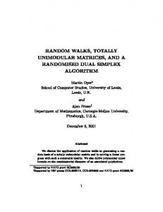
Figure 1: Recourse function for Example 2 approaches, the L-shaped method terminates to the same integer optimal solution if the solution is unique. However, if there are multiple optima, solving the master as a linear program may result in a non-integral solution, as the following example shows. Example 2 Suppose K = 2 and T 1 = T 2 = 1 and W 1 = W 2 = [1 − 1]. Clearly, the matrix B is TU by Proposition 9. Let c = 0 and d1 = d2 = [1 1]T . Hence, LP

Q

(x, k) =

(

hk − x x − hk

if x < hk , if x ≥ hk .

Suppose h1 = 1 and h2 = 2, each with probability 12 . Assume also 0 ≤ x ≤ 10. Because the first-stage objective cT x = 0, Q(x) is also the function z(x) to be minimized (see Figure 1). Suppose we start the L-shaped method at x1 = 0 and solve the master problem as a linear program. We show the sequence of iterations for the L-shaped method as follows. 1. Iteration 1: x1 is not optimal, generate the cut θ ≥ 1.5 − x. 2. Iteration 2: x2 = 10, θ2 = −8.5 is not optimal, generate the cut θ ≥ x − 1.5. 3. Iteration 3: x3 = 1.5, θ3 = 0 is not optimal, generate the cut θ ≥ 0.5. 4. Iteration 4: x4 = 1.5, θ4 = 0.5, which is optimal. It should be noted that with adding the last L-shaped optimality cut θ ≥ 0.5 to the master problem, the optimal solution x is not unique. As a result, solving the master problem as a linear program may not guarantee that the L-shaped method terminates with a feasible optimal solution to the totally unimodular stochastic program. However, as Theorem 10

10

shows, if an extreme point solution is obtained when solving the master problem at the last iteration of the L-shaped method, the first-stage decision must be integral. Let P M denote the polyhedral set of the feasible solutions (x, θ) of the master problem when the L-shaped method terminates. Theorem 10 Suppose the L-shaped method terminates with an optimal solution (x, θ) that is an extreme point of P M . Then if B is TU, x ∈ ZZn+1 . Proof: We will prove that the solution (x, y), with y = y LP (x), is an extreme point of P . The result then follows from the total unimodularity of B. Clearly (x, y) ∈ P . Suppose that (x, y) is not an extreme point of P . Then there exists (x1 , y 1 ) and (x2 , y 2 ) in P with (x1 , y 1 ) 6= (x2 , y 2 ) such that x =

1 1 x + 21 x2 2 1 2

and y =

1 1 y + 21 y 2 . 2

First, consider the case x1 = x2 = x. Then y 1 and y 2 (with y 6= y ) are feasible solutions to the linear program defining QLP (x) whereas y is an extreme point of the linear program 1 1 y 2

defining QLP (x). However, y =

+ 21 y 2 , and we have a contradiction.

Now, consider the case x1 6= x2 . Define θ1 =

PK

k=1

pk (dk )T (y k )1 and θ2 =

PK

k=1

pk (dk )T (y k )2 .

Note that (y i )T = ((y 1i )T , . . . , (y Ki )T ) for i = 1, 2. Then θ1 ≥ QLP (x1 ) and θ2 ≥ QLP (x2 ), and from the validity of the optimality cuts it follows that (x1 , θ1 ) ∈ P M and (x2 , θ2 ) ∈ P M . Moreover, 12 θ1 + 21 θ2 =

PK

k=1

pk (dk )T ( 21 (y k )1 + 12 (y k )2 ) =

PK

k=1

pk (dk )T y k = θ, where

the last equality follows from the fact that at termination of the L-shaped method θ = QLP (x) =

PK

k=1

pk (dk )T y k . We thus have (x1 , θ1 ) and (x2 , θ2 ) in P M , with x1 6= x2 such that

1 (x1 , θ1 ) + 12 (x2 , θ2 ) 2 M

of P .

= (x, θ). This contradicts the hypothesis that (x, θ) is an extreme point

2

Theorem 10 shows that one only needs to obtain an extreme point solution of the master problem as the L-shaped method terminates. This is normally ensured by using the simplex method for the master problem. Applying the L-shaped method to solve totally unimodular stochastic programs may not preserve the integrality property. Proposition 10 A master with at least one feasibility or optimality cut is in general not TU. Proof: In general, feasibility and optimality cuts contain coefficients not in {0, ±1}.

11

2

Theorems 8 and 9 indicate the trade-off of solving totally unimodular stochastic programs using the L-shaped method. On the one hand, Theorem 8 shows that a minimizer can be found in ZZn+1 . On the other hand, Theorem 9 shows that by solving the master as an LP, we are minimizing QLP (x), a convex function, over IRn+1 . Our computational experiments explore when this knowledge can be exploited.

5.

Computational Results Comparing Various L-shaped Approaches

As in the case of general stochastic linear programs with continuous second stage, the Lshaped method [19] can be used to exploit the dual block-angular structure existing in totally unimodular stochastic programs. While certain specialized versions of the L-shaped method may apply to certain classes of the problems, e.g., those with simple integer recourse [10], the purpose of our experiments is to explore the trade-off between the two approaches within the most common L-shaped method framework as described in Theorems 8 and 9. When applying the L-shaped method to totally unimodular two-stage stochastic programs, Theorem 8 and 9 indicate the trade-off in terms of solving the master problem. When integrality restrictions in X are relaxed, the master problem is easier to solve for a given set of cuts. However, in this case fractional solutions x may be generated. Since there exists an optimal solution with x being integral, solving the master over X may be advantageous, since every solution to the master is potentially an optimal solution. We solved four classes of totally unimodular two-stage stochastic programs. The first two classes of problems comprise instances in which T is a fixed TU matrix and W k is [I, −I] for each scenario k. The next two classes comprise instances in which T is identity matrix and W is a fixed TU matrix. Table 1 summarizes these four classes. We used the capacitated network generator NETGEN [8, 11] to generate TU matrices. Tables 2 and 3 show several parameters used in the TU matrix generation. In each class, we generated 100 totally unimodular stochastic program instances whose generating parameters are also reported in Tables 2 and 3. In Class 2, we specified that the second-stage objective function coefficients are the only stochastic component for simplicity in the generation. For each instance, we varied the number of scenarios, i.e., K = 1000, 2000, . . . , 10000, and tested two solution approaches in the L-shaped method. One approach was to solve the master problem itself as an IP at each iteration. The other one was to solve the LP-relaxation 12

Table 1: Characteristics of test problems 1st-stage 2nd-stage Class 1 MCNFP∗ Simple Recourse Class 2 Assignment Simple Recourse Class 3 Identity Matrix Assignment Class 4 Identity Matrix Transportation ∗ MCNFP: Multicommodity Network Flow Problem. Table 2: Generation of instances in Classes 1 and 2

T matrix # of # of Total Arc cost # of Class nodes arcs supply min max sources 1 40 65 30 1 10 2 70 100 35 1 20 35 2 ∗ h : average supply/demand generated by NETGEN. 0

SIP

# of sinks 2 35

2nd-stage obj ∼ U (5, 10) ∼ U (1, 10)

2nd-stage rhs ∼ U (0.9h0 , 1.1h0 )∗ 1

of the master problem at each iteration. All the instances were solved on a Pentium IV PC with a 2.40 GHz CPU and their computational results are reported in Tables 4 – 6. In Table 4, we present the average ratio of the number of cuts required by the approach of solving each master problem as an IP to the number of cuts required by the approach of solving each master problem as an LP. In Classes 1 and 2, only optimality cuts are needed since the stochastic integer programs have relatively complete recourse. Regardless of the number of scenarios, solving the master problem as an IP requires fewer cuts on average than solving its LP-relaxation. In Table 5, we present the number of integer incumbent solutions obtained in the L-shaped method with the approach of solving each master problem as an LP, for 10 instances randomly selected from Classes 3 and 4. These results show that the L-shaped method with the LP master approach converges along a much different path than the IP master approach. For some instances with given numbers of scenarios, e.g. Instance 1 from Class 3 with 1000 scenarios, it generates only one integer solution, namely the optimal solution. Since the generated fractional solutions are unlikely optimal, these results indicate that the LP master approach tends to require more iterations than the IP master approach. Table 6 reports the percentage of instances in which the approach of solving each master Table 3: Generation of instances in Classes 3 and 4

# of nodes Class 3 50 4 80 ∗ d : average arc 0

W matrix # of Total Arc cost arcs supply min max 90 25 1 20 300 500 1 10 cost genearated by NETGEN.

SIP

# of sources 25 40

# of sinks 25 40

13

1st-stage obj ∼ U (1, 20) ∼ U (1, 5)

2nd-stage obj ∼ U (0.5d0 , 1.5d0 )∗ ∼ U (0.5d0 , 1.5d0 )∗

Table 4: Average ratio for the number of cuts (LP master vs. IP master) Class 1 2 3

4

Cuts opt. opt. fea. opt. total fea. opt. total

1000 1.311 1.701 1.163 1.068 1.159 1.058 1.541 1.333

2000 1.304 1.695 1.151 1.149 1.164 1.083 1.543 1.347

3000 1.323 1.675 1.135 1.099 1.133 1.057 1.517 1.326

Number of 4000 5000 1.335 1.312 1.647 1.681 1.158 1.133 1.082 1.067 1.143 1.125 1.049 1.063 1.495 1.387 1.299 1.227

Scenarios 6000 7000 1.321 1.332 1.718 1.689 1.125 1.104 1.079 1.111 1.120 1.119 1.049 1.052 1.529 1.506 1.326 1.314

8000 1.300 1.653 1.149 1.122 1.153 1.049 1.515 1.323

9000 1.304 1.709 1.117 1.082 1.120 1.064 1.508 1.321

10000 1.271 1.715 1.157 1.112 1.151 1.072 1.536 1.340

Table 5: Integer incumbent solution in the L-shaped method with the LP master approach (# of integer incumbent solutions / # of iterations) Class

3

4

Instance 1 2 3 4 5 1 2 3 4 5

1000 1/61 5/52 1/56 1/43 1/41 3/185 3/154 2/164 1/144 7/119

2000 4/64 3/65 1/53 1/55 1/57 5/165 4/155 5/147 6/143 1/121

3000 5/57 1/62 1/47 1/47 2/42 4/178 3/162 8/156 3/141 6/117

4000 2/47 2/70 1/62 1/31 1/56 7/175 1/160 7/155 5/136 5/121

Number of Scenarios 5000 6000 7000 2/63 1/55 1/68 1/56 6/60 1/47 1/58 5/55 2/51 2/36 1/31 6/49 1/55 3/51 1/51 2/152 4/159 4/177 2/140 2/163 7/169 6/162 6/147 3/153 5/128 2/138 1/131 3/120 7/127 7/114

8000 1/68 2/54 2/51 1/33 2/56 5/163 2/160 5/160 2/136 9/132

9000 1/59 7/67 1/52 4/47 2/54 5/164 3/153 3/152 5/138 7/115

10000 2/61 2/60 2/57 1/36 4/59 6/163 12/165 6/154 1/128 11/132

problem as an IP takes less time than the approach of solving each master problem as an LP. In all four classes, solving the master as an IP is more likely to be superior as the number of scenarios increases. This observation can be interpreted as follows. When imposing the integrality restrictions on the master problem, the L-shaped method tends to require fewer iterations, which compensates the extra computational burden caused by solving the IP master. Table 6: Percentage of instances where solving IP masters is faster than solving LP masters Class 1 2 3 4

6.

1000 29 0 39 11

2000 51 10 56 33

3000 59 17 58 45

Number of Scenarios 4000 5000 6000 7000 69 69 73 78 20 28 33 37 60 56 58 58 58 61 72 71

8000 73 39 64 75

9000 75 47 62 79

10000 78 43 68 80

Conclusions

This paper considers two-stage stochastic programs with totally unimodular extensive-form constraint matrices. Such stochastic programs enjoy the integrality property in the sense that every extreme point solution is integral for any integer right-hand sides. 14

We provide sufficient conditions for a stochastic program to be totally unimodular. Our computational experiments explore under which conditions such stochastic programs should be solved with an integer master or a linear master. Our computational results indicate that when there are relatively few scenarios, solving an integer master is not worth the extra effort. However, as the number of scenarios grows solving fewer master problems becomes more important, and the IP master approach is more effective.

References [1] S. Ahmed, M. Tawarmalani, and N. V. Sahinidis. A finite branch-and-bound algorithm for two-stage stochastic integer programs. Mathematical Programming, 100(2):355–377, 2004. [2] J. R. Birge and F. V. Louveaux. Introduction to Stochastic Programming. Springer, New York, New York, 1997. [3] C. C. Carøe. Decomposition in stochastic integer programming. PhD thesis, University of Copenhagen, 1998. [4] G. B. Dantzig. Linear programming under uncertainty. Management Science, 1:197–206, 1955. [5] A. Ghouila-Houri.

Caracterisation des matrices totalement unimodulaires.

C. R.

Academy of Sciences of Paris, 254:1192–1194, 1962. [6] A. J. Hoffman and J. B. Kruskal. Integral boundary points of convex polyhedra. In H. W. Kuhn and A. W. Tucker, editors, Linear Inequalities and Related Systems, pages 223–246. Princeton University Press, 1956. [7] W. K. Klein Haneveld and M. H. van der Vlerk. Stochastic integer programming: General models and algorithms. Annals of Operations Research, 85:39–57, 1999. [8] D. Klingman, A. Napier, and J. Stutz. NETGEN: A program for generating large scale capacitated assignment, transportation, and minimum cost network flow problems. Management Science, 20:814–821, 1974.

15

[9] N. Kong, A. J. Schaefer, and B. K. Hunsaker.

Two-stage integer programs with

stochastic right-hand sides: A superadditive dual approach. To appear in Mathematical Programming, 2005. Available from Stochastic Programming E-Print Series (http://www.speps.info). [10] F. V. Louveaux and M.H. van der Vlerk. Stochastic programming with simple integer recourse. Mathematical Programming, 61(3):301–325, 1993. [11] MP-Testdata.

Capacitated

network

generator

Netgen.

Available

from

http://elib.zib.de/pub/packages/mp-testdata/generator/netgen/. [12] G. L. Nemhauser and L. A. Wolsey. Integer and Combinatorial Optimization. Wiley, 1988. [13] M. W. Padberg. Characterizations of totally unimodular, balanced and perfect matrices. In B. Roy, editor, Combinatorial Programming: Methods and Applications, pages 275– 284. Reidel, 1975. [14] A. Schrijver. Linear and Integer Programming. Wiley, 1986. [15] R. Schultz. Stochastic programming with integer variables. Mathematical Programming, 97(1-2):285–309, 2003. [16] S. Sen and J. L. Higle. The C 3 theorem and a D2 algorithm for large scale stochastic integer programming: Set convexification. Stochastic Programming E-Print Series, 2000. Available from http://www.speps.info. [17] L. Stougie. Design and analysis of methods for stochastic integer programming. PhD thesis, University of Amsterdam, 1987. [18] M. H. van der Vlerk. Convex approximations for complete integer recourse models. Mathematical Programming, 99(2):297–310, 2004. [19] R. Van Slyke and R. J-B. Wets. L-shaped linear programs with applications to optimal control and stochastic programming. SIAM Journal on Applied Mathematics, 17:638– 663, 1969. [20] R. Wollmer. Two stage linear programming under uncertainty with 0-1 integer first stage variables. Mathematical Programming, 19(3):279–288, 1980. 16