Towards Anytime Active Learning: Interrupting Experts to Reduce Annotation Costs Maria E. Ramirez-Loaiza
[email protected]
Aron Culotta
[email protected]
Mustafa Bilgic
[email protected]
Illinois Institute of Technology 10 W 31st Chicago, IL 60616 USA
ABSTRACT
incrementally while reading the document. In tumor detection by CT-scan, a radiologist forms an opinion as s/he spends more and more time on the images. In intrusion detection, a security analyst must inspect various aspects of network activity to determine whether an attack has occurred. We introduce a novel framework in which the active learner has the ability to interrupt the expert and ask his/her best guess so far. We refer to such a framework as anytime active learning, since the expert may be expected to return an annotation for an instance at any time during their inspection. For example, in document classification, we may show the expert only the first k words of a document and ask for the best guess at its label. We refer to a portion of an instance as a subinstance. Of course, the downside of this approach is that it can introduce annotation error — reading only the first k words may cause the annotator to select an incorrect label for the document. Assuming that both the cost to annotate an instance and the likelihood of receiving a correct label increase with the time the expert spends on an instance, the active learner has a choice on how to spend its budget: to collect either many but low-quality or few but high-quality annotations. Our active learning framework thus models the tradeoff between the cost of annotating a subinstance (a function of its size) and the value of the (possibly incorrectly labeled) instance. At each iteration, the algorithm searches over subinstances to optimize this tradeoff — for example, to decide between asking the human expert to spend more time on the current document or move on to another document. We build upon the value of information theory [6], where the value of a subinstance is the expected reduction in the generalization error after the instance is added to the training set. The subinstance with the highest value cost difference is shown to the expert for annotation. While previous work has considered the cost-benefit tradeoff of each instance [7] as well as annotation error [3], to our knowledge this is the first approach that allows the learning algorithm to directly control the annotation cost and quality of an instance by either interrupting the expert or revealing only a portion of an instance. Though closely-related, our framework differs from the missing feature-value acquisition problem [1, 10]; in our framework the feature values are not missing but the expert is interrupted. We perform experiments on three document classification tasks to investigate the effectiveness of this approach. In particular, we provide answers to the following research questions:
Many active learning methods use annotation cost or expert quality as part of their framework to select the best data for annotation. While these methods model expert quality, availability, or expertise, they have no direct influence on any of these elements. We present a novel framework built upon decision-theoretic active learning that allows the learner to directly control label quality by allocating a time budget to each annotation. We show that our method is able to improve performance efficiency of the active learner through an interruption mechanism trading off the induced error with the cost of annotation. Our simulation experiments on three document classification tasks show that some interruption is almost always better than none, but that the optimal interruption time varies by dataset.
Categories and Subject Descriptors I.5.2 [Pattern Recognition]: Design Methodology—Classifier design and evaluation
General Terms Algorithms, Experimentation, Human Factors, Measurement, Performance
Keywords Active learning, anytime algorithms, value of information, empirical evaluation
1.
INTRODUCTION
Active learning [2] seeks to reduce the human effort required to train a classifier. This is typically done by optimizing which instances are annotated in order to maximize accuracy while minimizing the total cost of annotations. In this paper, we begin with the simple observation that in many domains, the expert/user forms an opinion about the class of an instance incrementally by continuously analyzing the instance. For example, in document classification, the expert forms an opinion about the topic of the document
Permission to make digital or hard copies of all or part of this work for personal or classroom use is granted without fee provided that copies are not made or distributed for profit or commercial advantage and that copies bear this notice and the full citation on the first page. To copy otherwise, to republish, to post on servers or to redistribute to lists, requires prior specific permission and/or a fee. IDEA’13, August 11th, 2013, Chicago, IL, USA. Copyright 2013 ACM 978-1-4503-2329-1 ...$15.00.
RQ1. Annotation Error: Given that greater interruption can lead to greater annotation error, how do active learning algorithms perform in the presence of increasing amount of noise? We find that naïve Bayes consistently outperforms logistic regression and support vector machines as the amount of label noise increases, both in overall accuracy and in learning rate.
87
2.1
RQ2. Cost-Quality Tradeoff: Under what conditions is the cost saved by using subinstances worth the error introduced? How does this vary across datasets? We find that some interruption is almost always better than none, resulting in much faster learning rates as measured by the number of words an expert must read. For example, in one experiment, annotating based on only the first 10 words of a document achieves a classification accuracy after 5,000 words that is comparable to a traditional approach requiring 25,000 words. The precise value of this tradeoff is unsurprisingly data dependent.
We define the generalization error Err(PL ) through a loss function L(PL (y|x)) defined on an instance: Err(PL ) = E [L(PL (y|x)] Z = L(PL (y|x))P (x) x
1 X L(PL (y|x)) ≈ |U| x∈U A common loss function is 0/1 loss. However, because we do not know the true label of the instances in the unlabeled set U, we need to use proxies for the loss function L. For example, a proxy for 0/1 loss is:
RQ3. Adaptive Subinstance Selection: Does allowing the learning algorithm to select the subinstance size dynamically improve learning efficiency? We find that selecting the subinstance size dynamically is comparable to using a fixed size. One advantage of the dynamic approach is that formulating the size preference in terms of the cost of improving the model may provide a more intuitive way of setting model parameters.
L(PL (y|x)) = 1 − max PL (y j |x) yj
METHODOLOGY
In this section, we describe our methodology for the active learner that has the choice to interrupt the expert at any time. Let L = {(x1 , y1 ) . . . (xn , yn )} be a set of tuples containing an instance xi and its associated class label yi ∈ {y 0 , y 1 }. (For ease of presentation, we assume binary classification.) Let PL (y|x) be a classifier trained on L. Let U = {xn+1 . . . xm } be a set of unlabeled instances. Let xk ⊆ x be a subinstance representing the interruption of the expert at time k; or analogously the document containing the first k words in document x. For ease of discussion, we will use the document example in the remainder of the paper. Let Err(PL ) be defined as the expected loss of the classifier trained on L. The value of information for xki is defined as the reduction in the expected loss:
where p is the proportion of instances that are expected to be classified as class y 0 . This formulation requires us to know p, which is known approximately in most domains. In this paper, we use p = 0.5 by default, though this could be estimated directly from the training data. Note that when we use 0/1 loss proxy (Equation 3), the trivial solution of classifying all instances as y 0 with probability 1 achieves 0 error, whereas the ranked-loss for this trivial solution leads to an error of 1 − p. We leave for future work an empirical comparison of alternative loss functions.
V OI(xki ) = Err(PL ) − Err(PL∪(xi ,yi ) ) where L ∪ (xi , yi ) is the training set expanded with the label of xi , which is provided by the expert through inspecting xki . Because we do not know what label the expert will provide, we take an expectation over possible labelings of xki : X V OI(xki ) = Err(PL ) − PL (yj |xki )Err(PL∪(xi ,yj ) ) (1)
2.2
The Cost Function C(.) The cost function C(xki ) denotes how much the expert charges for annotating the subinstance xki . In practice, this cost depends on a number of factors including intrinsic properties of xi , the value of k, and what the expert has just annotated (the context-switch cost). To determine the true cost, user studies need to be conducted. In this paper, we make a simplifying assumption and assume that the cost depends simply on k. For documents, we can assume:
yj
Note that even though the expert labels only subinstance xki , we include the entire document xi in our expanded set L ∪ (xi , yj ). The decision-theoretic active learning strategy picks the subinstance that has the highest value cost difference: arg max V OI(xki ) − λC(xki )
(3)
One problem with this proxy in practice is that it trivially achieves 0 loss when all the instances are classified into one class with probability 1. We instead formulate another proxy, which we call rankedloss. The intuition for ranked-loss is that, in practice a percentage of instances are expected to belong to class y 0 whereas the rest are classified as class y 1 . Let p ∈ [0, 1] be the proportion of instances with label y 0 . Then, in U, we expect p × |U| of instances to have label y 0 and the remaining instances to have label y 1 . When we are computing the loss, we first rank the instances in U in descending order of PL (y 0 |xi ). Let this ranking be xr1 , xr2 , . . ., xr|U | . Then, ranked-loss is defined as: 0 1 − PL (y |xri ) if i < |U | × p (4) LRL (PL (y|xri )) = 1 − P (y 1 |x ) otherwise L ri
The rest of the paper is organized as follows: Section 2 presents our active learning framework, including implementation details and experimental methodology; Section 3 presents our results and provides more detailed answers to the three research questions above; Section 4 briefly summarizes related work; and Sections 5 and 6 conclude and discuss future directions.
2.
The Error Function Err(.)
C(xki ) = k or
(2)
C(xki ) = log(k)
xk i ⊆xi ∈U
where C(xki ) is the cost of labeling xki and λ is a user-defined parameter that translates between generalization error and annotation cost. We explain the role of this parameter in detail in Section 2.3. We next provide the details on how we define the error function Err(.), the cost function C(.), and the intuition for the parameter λ.
In this paper, we follow [7] and assume the annotation cost is a linear function of the instance length: C(xki ) = k.
2.3
The Parameter λ The value of information for xki is in terms of reduction in the generalization error whereas the annotation cost C(xki ) is in terms
88
of time, money, etc. The parameter λ reflects how much/little the active learner is willing to pay per reduction in error. Note that both 0/1 loss (Equation 3) and ranked-loss (Equation 4) range between 0 and 0.5, whereas the linear annotation cost is k. A λ value of 0.0001 means that for an x100 to be considered for i 100 annotation, V OI(x100 has to i ) has to be at least 0.01; that is, xi reduce the error by an absolute amount of 0.01. Typically, in the early iterations of active learning, improving the classifier is easier, and hence the range of V OI is larger compared to the later iterations of active learning. Therefore, the active learner is willing to pay less initially (because improvements are easy) but should be willing to pay more in later iterations of learning. Hence, a larger λ is preferred at the earlier iterations of active learning. Following this intuition, we define an adaptive λ that is a function of the current error of the classifier, Err(PL ):
We use this matrix to illustrate how our algorithm works as well as several baselines. At each iteration, our algorithm searches this entire matrix and picks the best candidate according to the objective function Equation 2. We refer to this method as QLT-γ (where γ is the desired percentage of improvement). Note that computing V OI for each candidate is computationally very expensive. We need to retrain our classifier for all possible labelings of each candidate. However, since a subinstance is only used for obtaining a label and we add xi (full instance) to L, therefore we only retrain our classifier once for each possible label of xi . That is, our algorithm has the same computational complexity as any V OI-based strategy. We define two baselines that ignore the cost of annotation. These approaches explore the candidates in C 0 by only searching at the fixed size column xki and selecting the best from that column. These approaches are:
λ = Err(PL ) × γ
• RND-FIX-k, a baseline, uses random sampling over candidates of size k. That is, random sampling elements of column k.
where γ is a fixed parameter denoting the desired percentage improvement on the current error of the model. For a fixed γ, λ is bigger initially because Err(PL ) is larger initially, and as the model improves, Err(PL ) goes down and so does λ.
2.4
• EER-FIX-k, a baseline that uses V OI over column k. Note that this is equivalent to expected error reduction (EER) approach (as described in [12]) on column k.
The Effect of Annotation Error
As discussed above, selecting small subinstances (equivalently, interrupting the expert after only a short time) can introduce annotation error. While previous work has proposed ways to model annotation error based on the difficulty of x or the expertise of the teacher [14], here the error is introduced by the active learning strategy itself. Rather than attempt to model this error directly, we observe that the objective function in Equation 2 already accounts for this error somewhat through the loss function. That is, if y ∗ is the true label of xi , then we expect Err(PL∪(xi ,y∗ ) ) < Err(PL∪(xi ,¬y∗ ) ). Note that the expanded training set includes the full instance, not simply the subinstance. This fact in part offsets inaccuracies in the term PL (yj |xki ) introduced by using subinstances. We study the empirical effect of this error in Section 3.
2.5
• RND-FULL and EER-FULL, baselines that use random sampling and expected error reduction (EER) respectively with full size instances. These approaches search on the last column of the matrix. Notice that once a fragment xki is selected as the best option for xi all other fragments of that document (i.e. row i) will be ignored.
2.6
2.6.1
Implementation Details and Baselines
Fixed
x10 1
10 x2 10 xi x10 n
x20 1 x20 2 x20 i x20 n
Full
...
xk1
...
x100 1
... .. . ... .. . ...
xk2
... .. . ... .. . ...
x100 2
xki xkn
x100 i x100 n
x1
Datasets
We experimented with three real-world datasets for text classification with train and test partitions; details of these dataset are available in Table 1. Reuters known as Reuters-21578 collection [8] is a collection of documents from Reuters newswire in 1987. We created a binary partition using the two largest classes in the dataset, earn and acq. SRAA is a collection of Usenet articles from aviation and auto discussion groups from [11]. For SRAA-Aviation dataset, we created a binary dataset using the aviation-auto partition. IMDB (movie) dataset is a collection of positive and negative movie reviews used in [9]. We preprocessed the dataset so that it is appropriate for a multinomial naïve Bayes. That is, we replaced all the numbers with a special token, stemmed all the words and eliminated terms that appear fewer than five times in the whole corpus. Stop words are not removed from the data to make sure the number of words the expert sees is similar to the number of words the model sees. We stress, however, that we kept the sequence of words in the documents, and that with the preprocessing the number of words did not change significantly. For example, the average document length before preprocessing in dataset Movie was 239 words and after preprocessing the average document length is 235 words.
In this section, we provide details on how we implemented our objective function Equation 2 and define a few baseline approaches. Let C = {x1 . . . xs } be a set of candidate instances for annotation, where C ⊆ U. We create a new set C 0 of subinstances xki from C. That is, our new search space includes xi and all subinstances derived from it. We use this new space to apply our objective Equation 2. We can illustrate the space defined by C 0 as a matrix where each row i allocates document xi and all its derived subinstances xk in ascending order of size. For simplicity, assume that k has increments of 10 words. The diagram illustrates the idea:
Experimental Evaluation
In this section, we first describe the datasets and then describe how we evaluated the aforementioned methods.
x2 xi xn
2.6.2
Evaluation Methodology
For the active learning results, we simulated interaction with real users by using a student classifier and an expert classifier — the expert classifier has the same form as the student, but is trained on more examples (and thus has higher accuracy). We experimented
89
3.1
Table 1: Description of the real-world datasets: the domain, the number of instances, and label distribution. Name IMDB Reuters SRAA - Aviation
Feat. 26,784 4,542 32,763
Train 25,000 4,436 54,913
Test 25,000 1,779 18,305
Total Inst. 50,000 6,215 73,218
Label dist. 50% 36% 37%
with the multinomial naïve Bayes (MNB) classifier implemented in Weka [5]. Moreover, we prefer MNB to simulate an expert since it intuitively simulates how a human expert works. For instance, a human annotator builds his/her belief about the label of a document as s/he reads it. That is, each read word builds evidence upon the previous ones read. Similarly, MNB builds evidence based on the terms that appear in a document to determine its classification. The default implementation of MNB uses Laplace smoothing. This implementation does not perform well for random sampling as well as active learning strategies in our datasets based on some preliminary experiments. We instead used informed priors where the prior for each word is proportional to its frequency in the corpus. Laplace smoothing is equivalent to create two fake documents, where each document contains every word in the dictionary exactly once. Informed priors is equivalent to creating two fake documents where every word appears proportional to its frequency in the corpus. This way, the prior will smooth more highly common terms to avoid accidental correlations that exist due to limited training data. For the purposes of this document when we refer to the classifier we mean this implementation unless otherwise stated. We used the original train-test partitions of the dataset. The test partition is used for only testing purposes. We further divided the original train split into two: half is used for training the expert model while the remaining half is used as the unlabeled set U. We performed two-fold validation in this fashion. Simulating Noisy Experts: Given the thousands of annotations required for our experiments, we propose a method to simulate the noise introduced by labeling document fragments. (We leave user studies to future work.) In each experiment, we reserve a portion of the data to train a classifier that will simulate the human expert. When a new annotation is required by the learning algorithm, the prediction of this classifier is used. To simulate annotation of a document fragment, we simply classify the document consisting of the first k words. We bootstrap all methods with two randomly chosen instances (one for each class). Then at each active learning step, we select randomly 250 unlabeled instances from U as candidates for labeling. The current loss and other computations needed by the methods are computed on a subset of 1000 unlabeled instances from the remainder of U (i.e. U \ Candidates). We evaluate performance on the test split of the dataset, report averages over the two folds and five trials per fold, and measure accuracy over a budget of number of words.
3.
RQ1. Annotation Error
Given that greater interruption can lead to greater annotation error, how do active learning algorithms perform in the presence of increasing amount of noise? To answer this question we designed an active learning experiment using different levels of label noise introduced in the training data. We tested Multinomial naïve Bayes with informed priors, L2 regularized logistic regression (LR) and support vector machines (SVM) implementation by LibLinear [4]. For the Label Noise Effect experiments, we create noisy data from the original training sets. We flipped the labels of 10% to 50% of the instances randomly. We evaluated using a train-test split repeating the experiment 10 times. Each experiment starts selecting two random instances (one for each class) and continues sampling randomly 10 instances at a time. We report the average over 10 trials. In our results we observed that for all classifiers the performance unsurprisingly decreases at greater levels of noise. Figure 1 shows the accuracy performance of the three classifiers on data with 10% and 20% label noise. All three classifiers performed better on datasets with 10% noise (Figure 1(a), Figure 1(b) and Figure 1(c)) compared to 20% noise (Figure 1(d), Figure 1(e) and Figure 1(f)). Similar results were found with greater levels of noise however we use only two examples for illustration. Interestingly, we observed that LR and SVM are more affected by the noise than MNB in particular at larger budgets. Moreover, MNB outperforms both LR and SVM at later iteration in the learning curve. This becomes more evident with greater percentages of noise. For instance, in Figure 1(b) MNB has a slower learning curve compared to LR and SVM whereas in Figure 1(e) MNB outperforms both classifiers half way through the learning curve. In general, with greater levels of label noise the performance of the tested classifiers gradually decreased. However, we find that MNB consistently outperforms LR and SVM as the amount of label error increases, both in overall accuracy and in learning rate, and so we use MNB in all subsequent experiments.
3.2
RQ2 - Cost-Quality Tradeoff
Under what conditions is the cost saved by using subinstances worth the error introduced? How does this vary across datasets? In Section 2, we proposed that expanding the search space to include subinstances could reduce annotation cost. Furthermore, we argue that it is possible to trade off the cost and the value of the information obtained from an instance. However, we still have to establish how the use of subinstances affects the learning performance of the model. In this section, we discuss our findings on the use of labeling subinstances instead of full instances. For this purpose, we tested the quality of the expert model training in one half of the data and tested showing the expert only the first k words of the documents. Also, we performed active learning experiments using random sampling and Expected Error Reduction (EER) as baselines testing subinstances of sizes 10 - 30 and 50. We followed the experimental methodology described in Section 2.6. Our results show that using full size instances was never a good strategy, performing similar to the random sampling baseline. Figure 2 shows that for all datasets EER-FULL and RND-FULL were about the same. However, in general, using subinstances improves the performance on the active learner model. We conclude that the tested model prefers to obtain numerous noisy labels rather than fewer high quality ones. For instance, Figure 2(a) shows RND-FIX-10 and RND-FIX-30 perform better than RND-FULLand EER--
RESULTS AND DISCUSSION
In this section, we analyze our empirical results to address the three research questions from Section 1. Since our interest is to find the best way to spend a budget and we focus on cost-sensitive methods, we analyze the performance of each method given a budget of the number of words an expert can read. We approach our discussion considering both performance measure and spending of the budget.
90
Accuracy - Movie with 10% Label Noise
Accuracy - Aviation with 10% Label Noise
Accuracy - Reuters with 10% Label Noise
0.90
0.75
0.90
0.85
0.70
0.85
0.80 0.80
0.60
0.75
Accuracy
Accuracy
Accuracy
0.65
0.70
0.55
0.75
0.70 0.65
0.50
0.65
0.60
LR-N10 MNB-N10 SVM-N10 0.45
LR-N10 MNB-N10 SVM-N10
LR-N10 MNB-N10 SVM-N10
0.55 0
500
1000 1500 Number of Documents
2000
0.60 0
(a) Movie - Effect of 10% Noise
500
1000 1500 Number of Documents
2000
0
(b) Aviation - Effect of 10% Noise
Accuracy - Movie with 20% Label Noise 0.75
0.65
0.70
1500
(c) Reuters - Effect of 10% Noise
Accuracy - Aviation with 20% Label Noise
0.70
500 1000 Number of Documents
Accuracy - Reuters with 20% Label Noise 0.80
0.75
Accuracy
Accuracy
0.65
Accuracy
0.60
0.55
0.60
0.50
0.55
0.70
0.65 LR-N20 MNB-N20 SVM-N20
LR-N20 MNB-N20 SVM-N20 0.45
0.50 0
500
1000 1500 Number of Documents
2000
LR-N20 MNB-N20 SVM-N20 0.60
0
500
1000 1500 Number of Documents
2000
0
500 1000 Number of Documents
1500
(d) Movie - Effect of 20% Noise (e) Aviation - Effect of 20% Noise (f) Reuters - Effect of 20% Noise Figure 1: Effect of Noise on the learning rate of several classifiers. MNB is less affected by label noise than LR and SVM. FULL on Movie dataset. Similarly, EER-FIX-10 and EER-FIX-30 outperform both random sampling counterparts. Furthermore, Figure 2(b) shows that with subinstances of size 10 the expert quality is only about 70%, more than 15 points bellow expert quality using full instances. Similar results were observed on Reuters dataset (see Figure 2(e) and Figure 2(f)). This set of results confirms those reported in the Section 3.1. In contrast, on Aviation dataset we observed that not all sizes of subinstances performed better than methods with full instances. In this case, EER-FIX-10 was worse than RND-FULL and EER-FULL whereas EER-FIX-50 outperformed all other methods. In general, we find that some interruption is almost always better than none, resulting in much faster learning rates as measured by the number of words an expert must read. For example, in Figure 3(a), annotating based on only the first 10 words of a document achieves a 65% accuracy after 5,000 words that is comparable to a traditional approach requiring 25,000 words. The precise nature of this tradeoff appears to vary by dataset.
3.3
by providing subinstances to the expert for labeling instead of full instances. However, the best subinstance size changes across dataset. For further exploration of this idea, we implemented the proposed Equation 2 as QLT-γ methods (see Section 2 for details). Our results suggest that the best value of γ depends on the budget. When the active learner’s budget is severely limited, a smaller γ, which is equivalent to many-but-noisy labels, is preferred, whereas when the budget is large, higher quality labels can be afforded. For instance, in Figure 3(a) QLT-γ = 0.01 performs better initially than QLT-γ = 0.0001 however the latter improves with larger budgets and has the same performance as QLT-γ = 0.01 in the end. Similar results are observed in Figure 3(g) for the same methods on Reuters. Furthermore, QLT-γ selects the size of the subinstance dynamically trading off cost and improvement. Figure 3(h) and Figure 3(b) show the average words per document for each method illustrating the dynamic approach of QLT-γ methods. Moreover, we observed different performances of the QLT-γ methods at different points of the budget spending. That is, expecting big improvements for larger budgets may not work best. For instance, Figure 3(i) shows that that QLT-γ = 0.01 works better at early iterations whereas QLT-γ = 0.0001 works better for later iterations. These differences are statistically significant as shown in Figure 3(i) where values below the 0.05 mark are statistically significant wins and above 0.95 are statistically significant losses.
RQ3 - Adaptive Subinstance Selection
Does allowing the learning algorithm to select the subinstance size dynamically improve learning efficiency? So far, we established a reference for the EER-FIX-k methods in terms of accuracy and how it translates to the budget efficiency. We have found that we can improve the budget efficiency
91
Accuracy – Movie – MNB Expert Quality 1.0
0.70
0.8
0.65
0.6 Accuracy
Accuracy
Accuracy - Movie - MNB with Fixed Subinstance Size 0.75
0.60
neg pos 0.4
RND-FULL RND-FIX-10 RND-FIX-30 EER-FULL EER-FIX-10 EER-FIX-30
0.55
Avg.
0.2
0.50
0.0 0
5000
10000 15000 20000 Number of Words
25000
30000
10
(a) Movie - Fixed Thresholds
ALL
(b) Movie - Expert Quality
Accuracy - Aviation - MNB w/ Fixed Subinstance Size
Accuracy – SRAA Aviation – MNB Expert Quality
0.95
1.0
0.85
0.8
0.75
0.6 Accuracy
Accuracy
30 50 70 100 Number of Words per Document
0.65
auto aviat. 0.4
RND-FULL RND-FIX-10 RND-FIX-50 EER-FULL EER-FIX-10 EER-FIX-50
0.55
Avg.
0.2
0.45
0.0 0
5000
10000 15000 20000 Number of Words
25000
30000
10
(c) Aviation - Fixed Thresholds
20 50 70 100 Number of Words per Document
ALL
(d) Aviation - Expert Quality
Accuracy - Reuters - MNB w/ Fixed Subinstance Size
Accuracy – Reuters – MNB Expert Quality
1.00
1.0
0.95 0.9 0.90 Accuracy
Accuracy
0.8 0.85
earn acq 0.7
RND-FULL RND-FIX-10 RND-FIX-20 EER-FULL EER-FIX-10 EER-FIX-20
0.80
0.75
Avg.
0.6
0.70
0.5 0
5000 10000 Number of Words
15000
10
20 50 70 100 Number of Words per Document
ALL
(e) Reuters - Fixed Thresholds (f) Reuters - Expert Quality Figure 2: Accuracy of fixed size subinstance baseline methods with MNB. On the right, expert quality of a MNB expert model tested on k words per document
The t-test results show that the tradeoff made by a big γ values with small budget compared to small γ for big budgets are significant. Based on this results, we conclude big γ selects mainly shorter subinstances which is beneficial for small budgets. On the other hand, small γ considers longer subinstances for labeling showing that for large budgets this works well.
Moreover, datasets that are more difficult to predict require a lower expected percentage of improvement for each word. That is, these datasets work better with smaller γ values where longer subinstances are considered also. That is the case of the Aviation dataset, considered a difficult dataset, where QLT-γ = 0.0005 performs better than QLT-γ = 0.001 and QLT-γ = 0.01. In
92
Accuracy - Movie - MNB with Adaptive Subinstance Size
Words per Document (Accum.) - Movie
0.75
T-Test - Reuters - QLT Methods vs. QLT-γ=0.01
10000
1.0 QLT-γ=0.0005 QLT-γ=0.0001 QLT-γ=0.01 EER-FULL EER-FIX-10 EER-FIX-30
0.70 1000
0.9
0.60 QLT-γ=0.0001 QLT-γ=0.0005 QLT-γ=0.01 EER-FULL EER-FIX-10 EER-FIX-30
0.55
p-value
0.8 Avg. Words per Document
Accuracy
0.65 100
0.7
10 0.6 QLT-γ=0.0001 QLT-γ=0.0005
0.50
1 0
5000
10000 15000 20000 Number of Words
25000
0.5
30000
0
(a) Movie - Accuracy
5000
10000 15000 20000 Number of Words
25000
30000
0
(b) Movie - Words per Document
Accuracy - Aviation - MNB w/ Adaptive Subinstance Size
15000 20000 Iterations
25000
30000
T-Test - Aviation- QLT Methods vs. QLT-γ=0.01
1000
0.5 QLT-γ=0.0005 QLT-γ=0.001 QLT-γ=0.01 EER-FULL EER-FIX-10 EER-FIX-50
0.90
100
QLT-γ=0.0005 QLT-γ=0.001 0.4
0.80
0.70 QLT-γ=0.0005 QLT-γ=0.001 QLT-γ=0.01 EER-FULL EER-FIX-10 EER-FIX-50
0.60
0.50
p-value
0.3 Avg. Words per Document
Accuracy
10000
(c) Movie - Significance Test
Words per Document (Accum.) - Aviation
1.00
5000
0.2 10 0.1
1 0
5000
10000 15000 20000 Number of Words
25000
30000
0.0 0
(d) Aviation - Accuracy
5000
10000 15000 20000 Number of Words
25000
30000
0
(e) Aviation - Words per Document
Accuracy - Reuters - MNB w/ Adaptive Subinstance Size
25000
30000
T-Test - Reuters - QLT Methods vs. QLT-γ=0.01
1000
1.0 QLT-γ=0.0001 QLT-γ=0.001 QLT-γ=0.01 EER-FULL EER-FIX-10 EER-FIX-20
0.95
0.90
10000 15000 20000 Number of Words
(f) Aviation - Significance Test
Words per Document (Accum.) – Reuters
1.00
5000
100
QLT-γ=0.0001 0.9
QLT-γ=0.001
0.8 0.7
QLT-γ=0.0001 QLT-γ=0.001 QLT-γ=0.01 EER-FIX-10 EER-FIX-20 EER-FULL
0.80
0.75
0.70
p-value
Avg. Words per Document
Accuracy
0.6 0.85
0.4 10 0.3 0.2 0.1 1
0
5000 10000 Number of Words
15000
0.5
0.0 0
5000 10000 Number of Words
15000
0
5000
10000 Number of Words
15000
(g) Reuters - Accuracy (h) Reuters - Words per Document (i) Reuters - Significance Test Figure 3: Comparison of fixed size subinstance methods and quality-cost adaptive subinstance size methods on a MNB classifier. On the center, the average words per document show the quality-cost methods dynamic selection of subinstance size compared to the fixed method. On the right, statistically significant p-value comparing QLT-γ methods
contrast, for an easy dataset such Reuters QLT-γ = 0.01 works best. As we have shown, selecting the subinstance size dynamically is comparable to using a fixed size. However, finding the best fixed k value is difficult and depends on the dataset, whereas γ = 0.0005 works reasonably well across datasets. Moreover, one advantage of the dynamic approach is that formulating the size preference in
terms of the cost of improving the model may provide a more intuitive way of setting model parameters.
4.
RELATED WORK
Although there are commonalities among other cost sensitive approaches and our proposed method, to our knowledge this is the first approach that allows the learning algorithm to directly influ-
93
ence the annotation cost of an instance by revealing only a portion of it. Feature value acquisition accounts for the value of asking questions to an expert and the expected improvement based on the answers such as the case of [1] and [10]. However, these formulations differ from ours since the feature values are known in our setting, but the expert is interrupted before the exert has the chance to fully inspect the instance. In scenarios where multiple experts provide noisy labels, the active learner has to decide how many and which experts to query. Zheng et al. [15] discuss the use of multiple experts with different cost and accuracy. Their approach concentrates on ranking and selecting a useful set of experts, and adjusts the cost of the expert based on the corresponding accuracy while the instances are sampled by uncertainty. Similarly, Wallace et al. [14] allocate instances to experts with different costs and expertise. Nonetheless, the main difference with the current scenario is that each instance is assumed to have the same cost given the expert. Furthermore, the active learner does not have control of either the cost or the quality of the labels and rather depends on the cost of the expert. Some decision-theoretic approaches incorporate cost into the active learning process by using linear cost function [7], or learning a cost model [3]. While these frameworks work well for their particular task, other studies report mixed results [13]. Instead, we propose an anytime active learning framework where the active learner balances cost and quality of labels by interrupting the expert labeling task.
5.
[3] P. Donmez and J. G. Carbonell. Proactive learning: : Costsensitive active learning with multiple imperfect oracles. In Proceeding of the 17th ACM conference on Information and knowledge mining - CIKM ’08, page 619, oct 2008. [4] R.-E. Fan, K.-W. Chang, C.-J. Hsieh, X.-R. Wang, and C.-J. Lin. LIBLINEAR: A library for large linear classification. Journal of Machine Learning Research, 9:1871–1874, 2008. [5] M. Hall, E. Frank, G. Holmes, B. Pfahringer, P. Reutemann, and I. H. Witten. The WEKA data mining software: An update. SIGKDD Explorations, 11, 2009. [6] R. A. Howard. Information value theory. IEEE Transactions on Systems Science and Cybernetics, 2(1):22–26, 1966. [7] A. Kapoor, E. Horvitz, and S. Basu. Selective supervision: Guiding supervised learning with decision-theoretic active learning. International Joint Conference on Artificial Intelligence (IJCAI), 2007. [8] D. D. Lewis, Y. Yang, T. G. Rose, and F. Li. Rcv1: A new benchmark collection for text categorization research. Journal of Machine Learning Research, 5:361–397, Dec. 2004. [9] A. L. Maas, R. E. Daly, P. T. Pham, D. Huang, A. Y. Ng, and C. Potts. Learning word vectors for sentiment analysis. In Proceedings of the 49th Annual Meeting of the Association for Computational Linguistics: Human Language Technologies, pages 142–150, Portland, Oregon, USA, June 2011. Association for Computational Linguistics.
FUTURE WORK
We have provided initial empirical evidence that expert interruption can lead to more efficient learning. All in all, our current set of results are important insight for anytime active learning algorithms that allow the learner to control and incorporate cost awareness. However, showing the first k words is only one way to interrupt an expert future directions include showing an automated summary of a document, showing selected sections of a document such as abstract and conclusion, etc. A future user study will provide additional insight. Another potential future direction include generalizing the anytime active learning framework to other domains, such as vision, besides text. Developing a general purpose active learning framework with anytime expert interruption is a promising new research direction.
[10] P. Melville, F. Provost, M. Saar-Tsechansky, and R. Mooney. Economical active feature-value acquisition through expected utility estimation. In Proc. of the KDD Workshop on Utilitybased Data Mining, 2005.
6.
[13] B. Settles, M. Craven, and S. Ray. Multiple-instance active learning. In Neural Information Processing Systems, pages 1289–1296, 2008.
[11] K. Nigam, A. McCallum, S. Thrun, and T. Mitchell. Learning to classify text from labeled and unlabeled documents. In Proceedings of the National Conference on Artificial Intelligence, pages 792–799, 1998. [12] N. Roy and A. McCallum. Toward optimal active learning through sampling estimation of error reduction. In International Conference on Machine Learning, pages 441–448, 2001.
CONCLUSION
Our main goal has been to design a framework that controls and accounts for cost and quality of training instances by means of interrupting an expert at any time during annotation. This interruption mechanism allows us to control the budget spending while improving the learning efficiency. We believe that this work can be extended to eliminate some of the assumptions and provide a better generalization to a broader range of domains.
[14] B. C. Wallace, K. Small, C. E. Brodley, and T. A. Trikalinos. Who should label what? instance allocation in multiple expert active learning. In Proc. of the SIAM International Conference on Data Mining (SDM), 2011. [15] Y. Zheng, S. Scott, and K. Deng. Active Learning from Multiple Noisy Labelers with Varied Costs. In IEEE 10th International Conference on Data Mining (ICDM), pages 639–648, 2010.
References [1] M. Bilgic and L. Getoor. Value of information lattice: Exploiting probabilistic independence for effective feature subset acquisition. Journal of Artificial Intelligence Research (JAIR), 41:69–95, 2011. [2] D. Cohn, L. Atlas, and R. Ladner. Improving generalization with active learning. Machine Learning, 15(2):201–221, 1994.
94