representation for unsupervised discovery of speech patterns. Com- ..... [2] A. Park and J. Glass, âUnsupervised pattern discovery in speech,â Trans. ASLP, vol.
TOWARDS MULTI-SPEAKER UNSUPERVISED SPEECH PATTERN DISCOVERY Yaodong Zhang and James R. Glass MIT Computer Science and Artificial Intelligence Laboratory Cambridge, Massachusetts 02139, USA {ydzhang,glass}@csail.mit.edu ABSTRACT In this paper, we explore the use of a Gaussian posteriorgram based representation for unsupervised discovery of speech patterns. Compared with our previous work, the new approach provides significant improvement towards speaker independence. The framework consists of three main procedures: a Gaussian posteriorgram generation procedure which learns an unsupervised Gaussian mixture model and labels each speech frame with a Gaussian posteriorgram representation; a segmental dynamic time warping procedure which locates pairs of similar sequences of Gaussian posteriorgram vectors; and a graph clustering procedure which groups similar sequences into clusters. We demonstrate the viability of using the posteriorgram approach to handle many talkers by finding clusters of words in the TIMIT corpus. Index Terms— unsupervised learning, language acquisition 1. INTRODUCTION Modern speech recognizers typically undergo a supervised training process with annotated speech data before they can be deployed on unseen test data. In our research we are interested in exploring speech processing approaches that can acquire information about the speech signal using unsupervised methods. There are many reasons why such approaches could prove beneficial for speech processing. Annotation of speech corpora is currently a very time consuming and expensive endeavor and is a limiting factor in how quickly speech recognizers can be created for new problem areas and languages. Given the relative ease of creating and storing large quantities of audio-visual speech material these days, methods that can process vast quantities of unannotated data to enable keyword search [1], audio summarization etc. could be quite useful. Finally, unsupervised methods might ultimately be effective as part of a larger speech recognition framework, especially if the structures they learn complement existing approaches. For example, our earlier research on unsupervised acoustic clustering was able to find clusters of re-occurring instances of spoken words [2]. Such independently-determined clusters could be useful for consistency checking of speech recognizer output. Although our earlier unsupervised acoustic pattern discovery work was effective in finding re-occurring instances of spoken words, it used Mel-Frequency Cepstral Coefficients (MFCCs) as the acoustic representation to perform pattern matching. It was not a problem for the task of academic lecture data that we have explored, since the majority of the lecture was recorded from a single talker. However, the natural question to ask was how we could generalize this procedure to handle multiple talkers. Although there are several techniques to transform the MFCC representation to a more speaker independent form (e.g., VTL [3]), in this paper, we describe our
recent research on replacing the MFCC-based representation with the Gaussian posteriorgram representation of the speech signal [4]. Instead of the usual MFCC vector, each frame is represented by a vector whose ith dimension indicates the posterior probability of being generated by the ith component of a Gaussian mixture model (GMM). The GMM itself is created in an unsupervised fashion on a large corpus of multi-talker data so that it models distributions of sounds across a variety of talkers. By using a representation that better accounts for the acoustic variation from multiple talkers, we show that the unsupervised clustering procedure can work better in a multi-talker environment. The new speech pattern acquisition approach is comprised of three steps: a Gaussian posteriorgram generation procedure which learns a GMM in an unsupervised way and labels each speech frame with a Gaussian posteriorgram representation; a segmental dynamic time warping (S-DTW) procedure which finds similar acoustic segments based on the distance defined on the Gaussian posteriorgrams; and a graph clustering procedure which groups the similar acoustic segments and outputs the final discovery results. While the last two procedures are essentially the same as our previous work [2], the first procedure differs substantially in how to represent speech frames. In the following sections we first describe the Gaussian posteriorgram concept, generation procedure, and review the segmental DTW and graph clustering methods. We then report our experience with clustering experiments we have performed on the multi-speaker TIMIT corpus, and provide some analysis of the behavior of the clustering algorithm. Finally, we discuss the results and suggest some plans for future work. 2. SPEECH PATTERN DISCOVERY 2.1. Gaussian Posteriorgram Definition The concept of the Gaussian posteriorgram is similar to the widely used posterior feature vectors [5]. Specifically, a Gaussian posteriorgram is a probability vector representing the posterior probabilities of Gaussian components in a GMM for a speech frame. Formally, if a speech utterance S contains n frames S = (s1 , s2 , · · · , sn ), then the Gaussian posteriorgram for this utterance is defined by GP (S) = (q1 , q2 , · · · , qn ). The length of qi is determined by the number of Gaussian components in the GMM, and each qi is calculated by qi = (P (C1 |si ), P (C2 |si ), · · · , P (Cm |si ))
(1)
where the j-th dimension in qi represents the posterior probability of the speech frame si on the j-th Gaussian component. m is the total number of Gaussian components.
Fig. 1. An illustration of segmental dynamic time warping between two utterances with R = 2. The blue and red regions outline possible DTW warping spaces for two different starting times. 2.2. Gaussian Posteriorgram Generation To generate Gaussian posteriorgrams, a GMM is trained on all speech frames without any transcription, and each frame is decoded by the trained GMM to obtain a raw posterior probability vector. Then, a discounting-based smoothing method is employed to each posterior probability vector to produce a Gaussian posteriorgram. In our work, each speech frame is represented by the first 13 MFCCs. After pre-selecting the number of desired Gaussian components, the K-means algorithm is used to determine an initial set of mean vectors. A GMM is then trained on all speech frames. Since we have observed uneven clustering results caused by the presence of noise and non-speech artifacts, we use a speech/non-speech detector to remove all non-speech segments longer than one second prior to clustering. Once a GMM is trained, a raw Gaussian posteriorgram vector is calculated by Equation 1. To avoid approximation errors, a probability floor is set to eliminate dimensions (i.e., set them to zero) with very small probability values. Then, a discounting based smoothing method is used to move a small portion of the probability mass from non-zero dimensions to zero dimensions. This smoothing helps during the time warping pairwise distance matching. 2.3. Segmental DTW Segmental dynamic time warping (S-DTW) has been successfully used in our prior speaker-dependent pattern discovery work [2] and in our recent unsupervised keyword spotting research [4]. After generating the Gaussian posteriorgrams for all speech utterances, S-DTW is performed on every utterance pair to find candidate cooccurring subsequences in the two utterances. To employ S-DTW, the difference function D between Gaussian posterior probability vectors p and q is defined as D(p, q) = − log(p · q). The dot product assumes these two probability vectors are drawn from the same underlying probability distribution. Given two Gaussian posteriorgrams GPi = (p1 , p2 , · · · , pm ) and GPj = (q1 , q2 , · · · , qn ), the warping function w(ik , jk ) can produce a m × n timing difference matrix, where ik and jk denote the k-th coordinate of the warping path. Two constraints are applied to the S-DTW search. One is the adjustment window condition that prevents the warping process from going too far ahead or behind in either GPi or GPj . Formally, an integer R is set to ensure |ik −jk | ≤ R. The other constraint is the step length condition. It is clear that the adjustment window condition restricts the shape and the ending coordinates of a warping path. Given different start coordinates, the difference matrix can be naturally divided into several continuous diagonal regions with width 2R + 1,
Fig. 2. Converting all matched fragment pairs to a graph. Each numbered node corresponds to a temporal local maximum in fragment similarity in a particular utterance (e.g., 1-5). Each matching fragment is represented by a connection between two nodes in the graph (e.g., 1-4, 2-4, 3-5).
as shown in Figure 1. The red warping region s2 denotes the warping process along with the j axis, while the blue warping region s3 denotes the warping process along the i axis. To avoid redundant computation and take into account warping paths across segmentation boundaries, an overlapped sliding window moving strategy is applied for the start coordinates, shown in the Figure 1. 2.4. Path Refinement By moving the start coordinate along the i and every � j axis, � �for � pair of speech utterances, we can obtain a total of n−1 + m−1 warpR R ing paths, each of which represents a warping between two subsequences in each utterance pair. Since our goal is to find sequences of similarity within the utterance pairs, we look for a fragment of each warping path that has a low distortion score [2]. The warping path refinement is done in two steps. In the first step, a length L constrained minimum average subsequence finding algorithm [6] is used to extract consecutive warping fragments with low distortion scores. In the second step, the extracted fragments are extended by including neighboring frames below a certain distortion threshold α. Specifically, we include neighboring frames with distortion scores within 1 + α percent of the average distortion of the original fragment. The reason is that we found that the path of extracted fragments often missed several frames at the onset or offset of a matching acoustic pattern (i.e., a particular word or words) [2]. 2.5. Graph Clustering After collecting refined warping fragments for every pair of speech utterances, we can try to cluster similar fragments. Since each warping fragment provides an alignment between two segments, if one of the two segments is a common speech pattern (i.e., a frequently used word), it should appear in multiple utterance pair fragments. The basic idea is to cast this problem into a graph clustering framework, illustrated in Figure 2. Consider one pair of utterances in which S-DTW determines three matching fragments (illustrated in different colors and line styles). Each fragment corresponds to two segments in the two speech utterances, one per utterance. Since in general there could be many matching fragments with different start and end times covering ever utterance, a simplification is made to find local maxima of matching similarity in each utterance, and to use these local maxima as the basis of nodes in the corresponding graph [2]. As a result, each node in the graph can represent one or more matching fragments in an utterance. Edges in the graph then correspond to fragments occurring between utterance pairs, with an associated weight that corresponds to a normalized matching score. After the conversion, a graph clustering algorithm proposed by Newman [7] is used to discover groups of nodes (segments) in terms of
graph distance. The role of the clustering algorithm is to decide which edges to group together, and which edges to eliminate. This latter point is especially important since it is possible to have partial overlapping matches ending at the same node that are essentially unrelated to each other. The clustering output is a list of disjoint groups of nodes which represent the underlying speech fragments. 3. EVALUATION To assess the behavior of the posteriorgram representation in a multitalker environment, we examined its performance on the TIMIT corpus. While TIMIT has some drawbacks for these purposes, we thought it would be a useful place to start since it has a small number of utterances from a relatively large number of talkers. The evaluation consists of two steps. In the first step, we examined the effects of the different setting of parameters for the S-DTW search and the path refinement. In the second step, we performed the graph clustering on the extracted S-DTW fragments using the best parameter setting obtained in step one. Using our distributed computing system (200 CPUs), it takes ten minutes to process one hour of speech data. 3.1. TIMIT Experiment Setup The TIMIT experiment was performed on a pool of 580 speakers (we combined the standard 462 speaker training set, and the larger 118 speaker test set). We excluded the dialect “sa” utterances since they were spoken by all speakers, and used the remaining 5 “sx” and 3 “si” utterances per speaker. A single GMM was created from all these data using 13 dimensional MFCC feature vectors that were computed every 10ms. Based on our recent experiments which used GMMs to represent speech [4], we computed 50 Gaussian components. Since TIMIT consists of read speech in quiet environment, the non-speech removal process was not applied. 3.2. Parameter Tuning Three main parameters in the S-DTW search and the path refinement were investigated. They were the adjustment window condition R, the length constraint L, and the path extension threshold α. The evaluation metric we used was the match rate of the path refinement output. After the path fragment refinement stage, a list of warping fragments is obtained. Each fragment corresponds to an alignment between two subsequences of frames in a pair of utterances. Based on the underlying orthographic transcription, we can represent each fragment by the closest matching underlying word sequence. A match rate between a set of fragments can then be calculated. Note that in this experiment, we were interested in finding speech patterns representing words or phrases. Therefore, the match rate was only calculated on fragments longer than 100 ms. We first examined the effect of using different S-DTW adjustment window sizes R, shown in the sub-figure (a) of Figure 3. We fixed the length constraint L = 500 ms and the path extension threshold α = 0.3. The results showed that a small S-DTW window size could overly restrict the warping path between two Gaussian posteriorgrams, while a big window size could relax the restriction too much and cause many problematic alignments. We found that a window size equal to 6 (i.e., 60ms) was the best choice, which was also the result we obtained in [4]. In sub-figure (b) of Figure 3, the length constraint, L, in the path refinement was changed from 400 ms to 600 ms while fixing R = 6 and α = 0.3. The choice of L = 500 ms appeared to be optimal.
Method MFCC GP
Table 1. TIMIT experiment results # Clusters Avg. Purity # Speakers 11 9.1% 457 264 79.3% 408
F/M 0.42 0.43
The result for the path extension threshold α is shown in the sub-figure (c) of Figure 3. α is varied from 0.1 to 0.5 while fixing L = 500 ms and R = 6. When α > 0.3, the match rate begins to fall. Therefore, we chose 0.3 as the best setting, which indicates a fragment is extended by including neighboring frames with distortion scores within 130% of the average distortion of the fragment.
3.3. Clustering Results and Analysis By setting R = 6, L = 500ms, and α = 0.3, we ran the graph conversion and clustering on the warping fragments from the path refinement output for both the original whitened MFCC representation and the Gaussian posteriorgram representation. The clustering result is shown in Table 1. MFCC represents the speaker dependent framework in with default settings (R = 5, L = 500ms, α = 0.1) [2]. GP stands for the Gaussian posteriorgram based method. Each cluster is given a purity score which represents the percent agreement of the underlying word label of each node in a cluster with the majority vote (e.g., a cluster with 2 nodes out of 4 with the same label would have a purity of 50%). From the table it is clear that the TIMIT task is very difficult for the original MFCC-based method due to the small number of utterances spoken by every talker, and the large number of talkers in the pool. The results did not change significantly when the clustering parameters were modified. Both the number of clusters that were automatically found, and the purity of the clusters increased substantially with the posteriorgram-based representation. Within each cluster, on average nearly 80% of the nodes agree with the majority word identity of the cluster. Since one of the properties we wished to explore was speaker variation, we also calculated the number of speakers covered by the clusters. The clusters determined using the Gaussian posteriorgram representation covered over 70% of the 580 speakers. Although the clusters obtained by the MFCC representation incorporated more speakers, the corresponding low purity score indicated that the clusters were fairly random. The gender ratio (Female/Male) of the entire corpus is 174/406=0.43, so it appeared that there was no obvious gender bias for the Gaussian posteriorgram method. Table 2 shows the top 5 clusters ranked by increasing average distortion score. The transcription column represents the word identity of the cluster. These top 5 clusters all have a purity score of 100% and they are all from different speakers. Note that since we ranked the clusters by distortion, the cluster sizes are small, even though we observed that several clusters had the same underlying word identity. Since the goal of this work was to demonstrate that the Gaussian posteriorgram representation can solve the multi-speaker case which our earlier work cannot handle, we leave the improvement of the clustering algorithm as future work. Another interesting point is that the top 5 clusters are identical for different parameter settings, which indicates that the phrases/words in each cluster are acoustically similar using the Gaussian posteriorgram representation. Since each “sx” sentence in TIMIT was said by seven talkers, we believe this contributed to the multi-word clusters that were observed, although the “si” data made up approximately 40% of the cluster data, which is the same proportion that it had in the overall corpus.
0.87
0.86
0.86
0.86
0.85 0.84 0.83 0.82 3
Match Rate (%)
0.87
Match Rate (%)
Match Rate (%)
0.87
0.85 0.84 0.83
4
5 6 S−DTW Window Size
7
8
0.82 400
0.85 0.84 0.83
450
500 550 Length Constraint
(a)
0.82 0.1
600
0.2
(b)
0.3 Alpha
0.4
0.5
(c)
Fig. 3. Fragment match rate for different parameter settings for the S-DTW and path refinement.
To better understand why using the Gaussian posteriorgram representation reduces the speaker variation issue, we calculated the alignment cost matrices of two speech segments of the word “organizations”, produced by a male and a female talker, respectively, using the S-DTW search, illustrated in Figure 4. The top and bottom sub-figures correspond to the cost matrix generated by MFCC and the Gaussian posteriorgram representation, respectively. The cost values were normalized into a grey scale for the purposes of the figure. The lighter the pixel is, the more similar the corresponding two frames are. The red line in each sub-figure corresponds to the is best-scoring alignment path. From the figures, it appears that on the MFCC-based representation, the cost values around the warping path show no strong difference from the values away from the warping path, especially at the end of the warping path. However, on the Gaussian posteriorgram representation, there is a better delineation between the low-cost alignment path and the region around the warping path. This observation suggests that the Gaussian posteriorgram representation is better modeling phonetic similarities across talkers, and is thus better able to make distinctions between phones. 4. CONCLUSION AND FUTURE WORK In this paper, we applied a Gaussian posteriorgram based approach to automatic acoustic pattern discovery in speech data. The entire acquisition process is completely unsupervised, and does not depend on speakers or languages. Compared with our previous work [2], the most important difference is that the Gaussian posteriorgrams are used to represent speech frames. The segmental dynamic time warping is then applied to speech frames represented by Gaussian posteriorgrams. By converting the warping results to a graph, a clustering algorithm is used to discover acoustic pattern clusters. On the TIMIT dataset, we successfully demonstrated the viability of our framework in a multi-talker environment. For future work, we plan to explore these clustering results on larger multi-speaker corpora. We also plan to more thoroughly ex-
Frames (mcth0)
3.4. Confusion Matrix Comparison
Cost Matrix 20 40 60 80
Frames (mcth0)
ID 1 2 3 4 5
Table 2. Top 5 clusters Cluster Size Avg. Distortion Transcription 2 0.87 shredded cheese 2 0.94 stylish shoes 3 1.02 each stag 3 1.06 the lack of heat 2 1.18 iris
20 40 60 80
10
20
30 40 50 Frames (fmju0) Cost Matrix
60
70
10
20
30 40 50 Frames (fmju0)
60
70
Fig. 4. Cost matrix comparison for a male and female speech fragment. plore the use of this framework on different languages. To date, we have performed some preliminary experiments on the OGI multilanguage dataset with encouraging results. 5. ACKNOWLEDGEMENTS The authors would like to thank T. J. Hazen for his insightful comments on this work. 6. REFERENCES [1] A. Garcia and H. Gish, “Keyword spotting of arbitrary words using minimal speech resources,” in Proc. ICASSP, 2006. [2] A. Park and J. Glass, “Unsupervised pattern discovery in speech,” Trans. ASLP, vol. 16, no. 1, pp. 186–197, 2008. [3] S. Demange and D. V. Compernolle, “Speaker nomalization for template based speech recognition,” in Proc. Interspeech, 2009. [4] Y. Zhang and J. Glass, “Unsupervised spoken keyword spotting via segmental DTW on Gaussian posteriorgrams,” in Proc. ASRU, 2009. [5] G. Aradilla, H. Bourlard, and M. Magimai-Doss, “Posterior features applied to speech recognition tasks with user-defined vocabulary,” in Proc. ICASSP, 2009. [6] Y. Lin, T. Jiang, and K. Chao, “Efficient algorithms for locating the length-constrained heaviest segments with applications to biomolecular sequence analysis,” J. Com. Syst. Sci., vol. 65, no. 3, pp. 570–586, 2002. [7] M. Newman, “Fast algorithm for detecting community structure in networks,” Phys. Rev. E, vol. 69, no. 6, 2004.