Towards Optimal Event Detection and Localization in Acyclic Flow Networks M. Agumbe Suresh, R. Stoleru, R. Denton, E. Zechman† , B. Shihada‡
!
Department of Computer Science and Engineering, Texas A&M University † Department of Civil Engineering, Texas A&M University ‡ Department of Computer Science, King Abdullah University of Science and Technology {agumbe,stoleru,denton,ezechman}@tamu.edu,
[email protected]
Abstract. Acyclic flow networks, present in many infrastructures of national importance (e.g., oil & gas and water distribution systems), have been attracting immense research interest. Existing solutions for detecting and locating attacks against these infrastructures, have been proven costly and imprecise, especially when dealing with large scale distribution systems. In this paper, to the best of our knowledge for the first time, we investigate how mobile sensor networks can be used for optimal event detection and localization in acyclic flow networks. Sensor nodes move along the edges of the network and detect events (i.e., attacks) and proximity to beacon nodes with known placement in the network. We formulate the problem of minimizing the cost of monitoring infrastructure (i.e., minimizing the number of sensor and beacon nodes deployed), while ensuring a degree of sensing coverage in a zone of interest and a required accuracy in locating events. We propose algorithms for solving these problems and demonstrate their effectiveness with results obtained from a high fidelity simulator.
1
Introduction
Acyclic flow networks are pervasive in infrastructures of national importance, including oil & gas and water distribution systems. Water distribution, one of seven critical infrastructure systems identified in the Public Health, Security, and Bioterrorism Preparedness and Response Act [1], is particularly vulnerable to a variety of attacks, including contamination with deadly agents through intentional or accidental hazards. Contamination of water supply can have acute consequences for public health and impact economic vitality [2]. To protect consumers in a network, water security measures should include an on-line, real-time contaminant warning system of sensors to quickly identify any degradation in water quality. Efficient placement of sensors is needed to collect information for responding to a threat by identifying the location and timing of the contaminant intrusion [3] and developing strategies for opening hydrants to flush a contaminant [4]. An extensive set of studies have been conducted to develop and apply optimization-based methodologies for placing sensors in a water distribution network [5] [6]. Due to the costs of placing and maintaining sensor networks, the sensor placement problem has been traditionally solved for a limited number of sensors that often cannot provide adequate coverage of a realistic network. In addition, existing sensor technology limits the locations for placing sensors, owing to a small number of points in an underground network that are both accessible and located near a power source. Recent research has investigated placement of wireless networks to enable a !
This publication is based in part on work supported by Award No. KUS-C1-016-04, made by King Abdullah University of Science and Technology (KAUST).
M. Agumbe Suresh, R. Stoleru, R. Denton, E. Zechman† , B. Shihada‡
2
new approach for monitoring water distribution systems through low-cost autonomous, intelligent sensor nodes. These systems have been preliminarily tested through deployment in municipalities and laboratory settings for detecting leaks and breaks in pipe networks [7] [8]. The research presented here provides the basis for exploring a new paradigm for monitoring acyclic flow networks in general, and water distribution systems in particular, through a set of mobile sensors. Mobile sensors can provide improved coverage of pipes and nodes at a lower cost to municipalities. Our research is enabled by recent advances in wireless sensor network technologies and successful deployments of, mostly static, sensor network systems for military applications [9], emergency response [10] and habitat monitoring [11]. In our proposed solution to the research challenges posed by accurate and inexpensive event detection and localization in acyclic flow networks, a mobile sensor network, consisting of mobile sensor nodes and beacons nodes is deployed in an area (i.e., distribution system) to be monitored. The sensor nodes are equipped with sensing modalities specific to the type of threat/event they need to detect. Once they are “inserted” into the flow network, they are moved by the flow along a set of fixed paths. For energy efficiency, reduced cost, and because GPS is not available, sensor nodes can only obtain their location by proximity to a set of fixed beacon nodes with known location. These sensors travel along the edges of the flow network, sensing and recording data, i.e. events and proximity to beacon nodes. Nodes may not possess communication capabilities (e.g., acoustic modems), for costs and form factor reasons (if nodes can not communicate, their physical capture will be needed). Using the data collected by sensor nodes we aim to identify the existence and location of an event. This research addresses the problem of reducing the number of sensors and beacon nodes deployed in an acyclic flow network, while ensuring that a desired accuracy of event detection is achieved. More specifically, the contributions of this paper are as follows: – We propose the idea of acyclic flow sensor networks, and formally define the problems for optimal event detection and localization in such networks. – We prove that the event detection problem is NP-Hard and we propose an approximation algorithm to derive the minimal number of sensor nodes to be deployed and their deployment locations. – We propose algorithms for optimally solving the Event Localization problem in acyclic flow networks, through an intelligent deployment of beacon nodes. – We evaluate the performance of our solutions through extensive simulations using a high fidelity acyclic flow network simulator. The rest of the paper is structured as follows. In Section 2 we formulate the problem of optimal event localization in acyclic flow networks, and Sections 3 and 4 propose solutions for it. We present performance evaluation results in Section 5 and review state of art in Section 6. We conclude in Section 7 with ideas for future work.
2
Preliminaries and Problem Formulation
An acyclic flow network can be best understood by considering a typical example - a water distribution system, as shown in Figure 1. Water, stored in water reservoirs or water towers, is pumped by pumpstations into a network of underground pipes. Depending on the demand of water by various consumers, the flow in pipes can change in direction and magnitude. In a water distribution system, we are interested in identifying the point(s) in the system where an attack, e.g., chemical contamination, might be taking place. To achieve accurate and cost effective
Towards Optimal Event Detection and Localization in Acyclic Flow Networks
3
discovery of the contamination point, we propose to deploy sensor nodes, equipped with suitable sensors (i.e., chemical sensors in our scenario) in the water distribution system. Due to unavailability of GPS underground, a deployed sensor node can only infer its position from its proximity to points with known locations, such as beacon nodes. In this paper, we assume the availability of inexpensive sensor nodes, equipped with simple sensing modalities and with no communication capabilities. Simple sensing modality means that the sensor is capable of detecting contamination in large concentrations only, i.e., typically around the point of contamination. The lack of communication capabilities means that sensor nodes do not collaborate. In this paper, for deriving optimal event localization algorithms, Fig. 1. An acyclic flow network example we consider time-invariant flow networks, in which the flow - a water distribution system, encompassdoes not change in time. ing water storage (e.g., reservoir and waIn the remaining part of this section we formally define ter towers), and water distribution (i.e., a terms pertaining to acyclic flow networks and formulate network of underground pipes). the optimal event detection and optimal event localization problems. 2.1
Definitions
We consider a directed acyclic graph G(V, E) in which every edge (u, v) ∈ E has a non-negative, real-valued capacity denoted by c(u, v), and two sets of vertices: S = {s1 , s2 , ..., sk } a set of sources, and D = {d1 , d2 , ..., dk } a set of sinks, where S, D ⊂ V . Definition 1. An Acyclic Flow Network, F, is defined as a real function F : V × V → R with the following properties: – F(u, v) ≤ c(u, v), where c(u, v) is a constant. This means that the flow on an edge, cannot exceed its capacity.! ! – w∈V F(u, w) = w∈V F(w, u)∀u ∈ V , unless u ∈ S or w ∈ D, which means that the net flow of a vertex is 0, except for source and sink nodes. Definition 2. A Beacon Node (Bi ) is a node which periodically broadcasts its location. A beacon node is placed at a vertex vj ∈ V . Definition 3. A Sensed Path (SPi ) is a set {ej | ej ∈ E} of edges through which a node ni traveled and sensed events and proximity to beacon nodes. Definition 4. An Insertion Point (or Source) for a node ni is a vertex vj ∈ V at which the node is introduced into the flow network. Definition 5. A Path Synopsis (P Si ) for a node ni is an ordered list of events and beacons encountered by node ni along its Sensed Path SPi . Definition 6. A Zone of Interest (I) is a subset of edges in graph G(V, E), i.e., I ! E, which we are interested in monitoring. A given F can have multiple zones of interest.
4
M. Agumbe Suresh, R. Stoleru, R. Denton, E. Zechman† , B. Shihada‡
Definition 7. The Degree of Coverage (Dc ) is the fraction of I that nodes need to sense/traverse. More precisely, 0 ≤ Dc ≤ 1, and at least Dc of edges in I are being traversed by sensor nodes. Definition 8. The Probability of Detection / Event Localization Accuracy (Pd ) is the probability of finding an event (or the accuracy of event localization) in Zone of Interest I. Formally, (T P +T N ) Pd = (T P +T N +F P +F N ) , where TP, TN, FP and FN are true positives (i.e., an event existed and the algorithm detected it), true negatives (i.e., an event did not exist and the algorithm correctly indicated a non-existence), false positives (i.e., an event did not exist, but the algorithm detected one) and false negatives (i.e., an event existed and the algorithm failed to detect it), respectively. Definition 9. A Suspects List is the list of edges {ei | ei ∈ E} in which an event of interest was detected by a sensor node (i.e., recorded in its Path Synopsis). 2.2
Formulations of Problems
Given the above definitions, an Acyclic Flow Network poses two interesting problems. The first one is the “Optimal Event Detection Problem”, i.e., detecting the existence of an event in a zone of interest, using the least resources possible. This problem is a binary decision, i.e., an event is present or not. The second problem is the “Optimal Event Localization Problem”, i.e., detecting the location of an event, using the least resources possible. From here on we will refer to “Event Detection” as “Sensing Coverage”, since detecting an event requires sensing coverage. The two aforementioned problems are formally defined as follows: Optimal Event Detection (Sensing Coverage) Problem (SCP): Given an acyclic flow network F, a zone of interest I in F, and degree of coverage Dc , find the smallest set S = {(si , qi ) | si ∈ V ∧ qi ∈ N} of insertion points si (sources) where sensor nodes need to be deployed, and the smallest number qi of sensors to be deployed at si , such that the union of sensed paths of all sensors represents at least Dc of I. Optimal Event Localization Problem: Given an acyclic flow network F, a zone of interest I in F, with required probability for detecting an event Pd , compute the minimum number of beacon nodes that need to be deployed in F, and their deployment locations (i.e., vertices in V ) such that !|S| from {P Si | i ≤ i=1 qi } (a set of path synopses) for all sensor nodes deployed in the F, the probability of localizing an event X, detected by sensor nodes, by identifying a set of edges where the event could be present (i.e. Suspects List) is Pd . It is important to build the intuition that Dc determines the number of nodes to be inserted in the flow network (i.e., sensing coverage for event detection), whereas Pd determines the number of beacons to be deployed (event localization accuracy). When Pd is high most vertices in the flow network will have beacons. So, even if the sensing coverage of zone of interest is small, if an event is detected it is localized more accurately when Pd is high (note that Pd is high and Dc is low, there is a chance that an event might not be detected). Typically, ensuring sensing coverage is less important than accurate event localization. In systems where it is sufficient
B4 v1
v2
B1 v6
B3
X
v5
v4
v8
B2 v3
v7
B5
I
Fig. 2. Graphical representation of an acyclic flow network involving vertices/junctions, edges/pipes, and defined elements for the event detection problem: a zone of interest I, beacon nodes Bi and an event X along edge (v5 , v4 ).
Towards Optimal Event Detection and Localization in Acyclic Flow Networks
5
to know that an event occurred, Pd can even be 0, which means no beacons are required. Example 1: For clarity of presentation, we illustrate the aforementioned concepts with an example, depicted in Figure 2. In the shown acyclic flow network, the Zone of Interest I consists of 6 edges, (v1 , v2 ), (v1 , v5 ), (v8 , v5 ), (v5 , v4 ), (v7 , v4 ) and (v8 , v7 ) (i.e., this is the area where events of interest might occur), and the Degree of Coverage Dc is 0.67, i.e., any four of the six edges of I must be sensed/traversed. Five beacon nodes (B1 , B2 , B3 , B4 and B5 ) are deployed to ensure a Pd of 0.67, and a number of sensor nodes are deployed at the Insertion Point vertex v6 . A node ni might travel along edges (v6 , v1 ), (v1 , v5 ), (v5 , v4 ) and (v4 , v3 ) (i.e., a Sensed Path SPi ). Consequently, the Path Synopsis for node ni is P Si = {B1 , B4 , X, B3 , B2 }. A solution for event localization is a set of edges, i.e., “Suspects List”, where the event might be present: = {(v1 , v5 ), (v5 , v4 )}.
3
Node Placement for Optimal Sensing Coverage
We first show that SCP reduces to the Weighted Set Cover problem, a known NP-Hard problem. Theorem 1: SCP is NP-Hard. Proof. Take an instance of the Weighted Set-Cover (WSC) problem (E, V, S, w) where: E = {ei | i = 1, 2, . . . , n} V = {Vj | j = 1, 2, . . . , m; Vj ⊆ E}; S⊂V|
"
Vj ∈S
m "
j=1
Vj = E
Vj = E
ω:V→R # W = ωj Vj ∈S
where E is a set of elements, V is a set of subsets of E covering all elements of E, S is a subset of V that contains all elements of E. Each subset Vj has a weight ωj . S is constructed such that E can be covered with cost W . We construct f : WSC → SCP V = {wj | j = 1, 2, . . . , m} ∪ {ui | i = 1, 2, . . . , n} ∪ {vi | i = 1, 2, . . . , n} E = E1 ∪ E2 where E1 = {(wj , ui ) | ei ∈ Vi }; E2 = {(ui , vi ) | i = 1, 2, . . . , n} I = E2 ; D c = 1
F(u, v) =
c(u, v)
|Vi | ωi
0
if (u, v) ∈ E2 if (u, v) ∈ E1 if (w, u) ∈ / E1 but (u, v) ∈ E2
where V , E, I, and Dc represent the vertices, edges, zone of interest and degree of coverage of FSN, respectively, and F(u, v) is the flow in edge (u, v). I can be covered with W sensor nodes.
6
M. Agumbe Suresh, R. Stoleru, R. Denton, E. Zechman† , B. Shihada‡
Note that V is constructed in O(m) time, E and I in O(n + m) time, F in O(n + m) time and Dc in constant time. Hence, this construction occurs in polynomial time. Equivalence: S covers E with cost W ⇐⇒ Dc of I in F can be covered by W sensor nodes. ⇒ Given S covers E with cost W . Since Dc = 1, all edges in I need to be covered. The number of nodes to be inserted in wj , j = 1, 2 . . . m such that all edges incident on it are covered is ωj | j = 1, 2 . . . m. Any node that reaches ui will cover the edge (ui , vi ). Since S covers E with cost W , selecting the corresponding vertices in F covers all edges in I. So, if S covers E with cost W , inserting W sensor nodes in the corresponding vertices in F, Dc of I will be covered. ⇐ Given Dc of I in F can be covered by W sensor nodes. By our definition of E, all ui ’s are covered by at least one wj . Hence, any set of ui in the set of insertion points can be replaced by an existing wj without increasing the cost. Notice that using our definition of E, each vertex wj can be used to uniquely identify Vj ∈ V. Further, each wj covers a set of edges in I and each corresponding Vj covers a set of elements in E. So, the sets corresponding to the insertion points ensure that V covers E with cost W . In the remaining part of this section we present a heuristic solution for SCP.
3.1
Optimal Sensing Coverage Algorithm
The algorithm we propose for solving the optimal sensing coverage problem, depicted in Algorithm 1 consists of three main steps: in the first step we derive the number of sensor nodes that must be deployed at each vertex, such that edges in the zone of interest are covered (this step is reflected in Lines 1-8); in the second step we derive the minimum number of nodes required to ensure Dc coverage of zone of interest (this step is reflected in Lines 9-15); in the third step we obtain the best insertion points for the mobile sensor nodes (this step is reflected in Lines 16-26)). These steps are described in detail below. In order to ensure sensing coverage we first derive the probability that a sensor node deployed in an acyclic flow network F will reach a zone of interest. The simplest case is when we have a single source in the acyclic flow network and the sensor nodes are inserted at this source. In this case, the probability pi that a single node will traverse a particular edge in F is pi = Tffi , where fi is the network flow in edge i and Tf is the total network flow (i.e., inserted at all source vertices). In a multiple source F, where we allow sensor nodes to be inserted at any vertex, we derive pi using a matrix M,
Algorithm 1 Sensing Coverage Require: Dc , F 1: for each ei ∈ E do 2: for each ej ∈ E do 3: Mij = prob(ei , ej ) 4: end for 5: end for 6: while Mk "= 0 do 7: T+ = Mk ; k + + 8: end while 9: for each ei ∈ E do 10: for each ej ∈ E do 11: i! = ei .terminal vertex; 12: j ! = ej .terminal vertex ln(1−Dc ) 13: Ni! ,j ! = ln(1−T +1 ij ) 14: end for 15: end for 16: for each!ei ∈ V do N.row(i)+max(N.row(i)) 17: gi = (num non zero(N.row(i)))α 18: end for 19: while g "= 0 do 20: i = min(g) 21: S+ = {vi , max(N.row(i))} 22: for each ej covered by vi do 23: j ! = ej .teminal vertex 24: N i, j ! = 0 25: end for 26: end while
Towards Optimal Event Detection and Localization in Acyclic Flow Networks
that describes the edge to edge transitions as follows: 0 e12 e21 0 M= ... ... e(|E|+r)1 e(|E|+r)2
7
... e1(|E|+r) ... e1(|E|+r) ... ... ... 0
where eij is the probability that a sensor node currently in edge i will be in edge j after passing through the next vertex (i.e., the rows of M represent the current edge and the columns of M represent the next edge, after passing through a vertex) and r is the number of source vertices in the flow network (to account for node insertion into the flow network, we add one fictitious edge to each source node). In Lines 1-5 of Algorithm 1, this matrix is constructed. The prob function in Line 3 calculates the probability that a sensor node currently in the edge ei will be in the edge ej after passing through the next vertex. The probabilities that a node inserted in F will traverse a particular edge are computed in the form of a “traversal probability matrix” T, as follows: T=
p #
k=1
Mk , such that Mp = 0|E|+r,|E|+r
(1)
where 0|E|+r,|E|+r is the zero matrix of size |E| + r, |E| + r. In T , as defined in Equation 1, tij is the probability that a sensor node inserted into the edge i will traverse edge j of F. Because F is acyclic, to compute the probability that a node inserted traverses a particular edge, we need to consider a p large enough such that Mp is a zero matrix (i.e., all sensor nodes have reached sink vertices). Lines 6 - 8 of Algorithm 1 construct the matrix T using M. Derivation of Number of Nodes Required for Dc (Step 2) To determine νi - the number of nodes needed to achieve detection threshold Dc on edge ei , we first define a random variable X for the number of sensor nodes that pass through the edge ei . Next, notice that X will follow a binomial distribution b(n, p), thus it is described by the probability mass function: - . n x f (x) = p (1 − p)n−x , x = 0, 1, . . . , n (2) x Let’s define an event A when at least one sensor node passes through an edge ei . We aim to determine νi (the number of sensor nodes needed to reach the detection threshold Dc ) such that P (A) ≥ Dc . Note that P (A) = 1 − P (A# ), where A# is the complement of A, making P (A# ) the probability that no node will traverse the edge ei . Using Equation (2) we obtain: P (A) = 1 − P (A# ) = 1 − (1 − pi )νi ≥ Dc From Equation (3), νi can be obtained as: / 0 ln(1 − Dc ) νi ≥ ln(1 − pi )
(3)
(4)
When the probability pi of reaching an edge is known we can then calculate the number of sensor nodes that need to be inserted to reach a desired detection threshold Dc . If pi ≥ Dc then
8
M. Agumbe Suresh, R. Stoleru, R. Denton, E. Zechman† , B. Shihada‡
one sensor node is sufficient for detection. When pi < Dc then a larger number of nodes need to be inserted to reach the detection threshold. Using Equation (4) the traversal probability matrix T is converted to a “node requirement matrix” N, in which each element ni! j ! is the number of nodes to be inserted into the ith edge’s terminal vertex vi! to reach jth edge’s terminal vertex vj ! with probability Dc . Formally, N is defined as: n11 ... n1|V | N = ... nij ... n|V |1 ... n|V ||V | 1 2 c) # # where ni! j ! = max(ni! j ! , ln(1−D ln(1−tij ) ) where vi is the terminal vertex of ei and vj is the terminal vertex of ej . Wherever an element of T is 0 (i.e. the destination edge is not reachable from the insertion edge,), a 0 is also present in N, as a marker for unreachability. This formalism allows each edge to have a different detection threshold by applying different values of Dc to each column of T. This may be useful in cases where detection in some edges is much more important than others. Lines 9-15 of Algorithm 1 construct N using T and the binomial distribution equation 4. To obtain a solution for our sensing coverage problem we must select a set of “good” insertion points from the matrix N that cover our zone of interest in the flow network. Insertion Point Selection Heuristic (Step 3) Since our problem is NP-hard, we define a “goodness” metric g, to allow our algorithm to make a greedy choice. We define g as: (ri + rm ) where i = 1, ..., |V | (5) #α ! where ri is the sum entries in row i of N (i.e., rs = j nij ), rm is the maximum element of N, # is the number of non-zero elements in the row of N, and α is a tuning parameter that allows us to control the importance of coverage in calculating gi . For a single source acyclic flow network, a lower value of α may be necessary to pull focus away from the source vertex. Each vertex now has a corresponding goodness value, based on N. The goodness vector is constructed using the goodness metric in Lines 16-18 of Algorithm 1. The smallest gi corresponds to the best vertex vi (i.e., gi relates to the number of nodes to be deployed to cover each edge). By reducing this number, we ensure that as few nodes as possible are inserted. The maximum element in the ith row of N is the number of nodes to be inserted at vi . The smallest value of gi is chosen from g in Line 20. In Line 21, that vertex is added to S, where si is the vertex vi and qi is the maximum element in row i of N. Finally, vertices covered by vi are removed from N in lines 22-25. This process is repeated, selecting vertices until a coverage threshold is met or until N = 0, which indicates that all remaining vertices are unreachable. We then select si = vi and qi = max(N.row(i)) to obtain {si , qi } to be inserted into set S. When the algorithm terminates, it produces a set of vertices, each with an associated number of nodes to be inserted into the flow network, that meet the sensing coverage requirement. gi =
Algorithm Complexity: This greedy heuristic is an approximation to the optimal solution for node placement in a FSN. The heuristic uses the same technique used to approximate the weighted set cover problem. The approximation ratio for this heuristic was proved to be ln |V | [12]. The flows in all the edges is known, so Line 3 takes O(1) time. So, Lines 1-5 take O(|E|2 )
v3
e2 v1
e1
v2
e3
e4 v4
Fig. 3. Graph example
Towards Optimal Event Detection and Localization in Acyclic Flow Networks
9
time. Time complexity of calculating Mi × M to get Mi+1 is O(|E|3 ). So, Lines 6-8 take O(|E|3 p) time. Construction of N using T and the binomial distribution equation 4 takes time O(|E|2 ). The goodness vector is constructed using the goodness metric in time O(|V |). Choosing the vertices in Lines 19-26 takes O(|V |2 ) The most time consuming step in the algorithm is the construction of the Traversal Probability Matrix, the time complexity of the Sensing Coverage Algorithm is O(|E|3 p). Asymptotically, this is O(|E|3 ). Example 2: For clarity of presentation we exemplify how our algorithm works for a flow network shown in Figure 3, where we let the flow be equally divided in edges e2 and e3 . e1 is a virtual edge added to introduce incoming flow into the network. So, the traversal probability matrix T derived from Equation 1, and the node requirement matrix N with a Dc of 0.75, as defined in Equation 4 and the goodness vector when α = 2 derived from Equation 5 will be: 0 0.5 0.5 0 0 0.5 0.5 0.5 0000 0 0 0 1 0 0 0 1 0 0 2 2 3 4 M= (6) 0 0 0 0 ; T = 0 0 0 0 ; N = 0 0 0 1 ; g = ∞ 1.5 2 ∞ 0 0 0 0 0 0 0 0 0000 Now, vertex v2 is chosen since it has the smallest g. The maximum element in the second row of N is 2. Hence 2 nodes are inserted at vertex v2 . All edges reachable from v1 are removed from N. This reduces the matrix to a zero matrix. Hence, we obtain S = {v2 , 2}. Since e1 was a virtual edge, this ensures that at least Dc edges are covered.
4
Beacon Placement for Optimal Event Localization
Our solution for the problem of optimal event localization in acyclic flow networks consists of two steps: in the first step we seek an optimal placement of beacon nodes (i.e., reduce the number of beacon nodes); in the second step, using the path synopsis collected from sensor nodes, we identify the location of an event. More formally, these steps are described as follows: i) Beacon Placement Algorithm: given F - an acyclic flow network and Pd - the required accuracy of event localization, find the set B = {bi | bi ∈ V } of vertices where beacon nodes are to be placed such that the probability of finding an event is greater than Pd ; ii) Event Localization Algorithm: given F - an !|S| acyclic flow network and {P Si | i ≤ i=1 qi } - a set of path synopses for all sensor nodes deployed in the F, localize an event X, detected by sensor nodes, by identifying a set of edges, i.e. Suspects List, where the event might be present. In the remaining part of this section, we present our algorithms for solving the optimal event localization problem. 4.1
Beacon Placement Algorithm
The Beacon Placement algorithm is presented in Algorithm 2. This algorithm optimizes the placement of beacon nodes in the network, so that the event localization algorithm can achieve a Pd accuracy. The algorithm uses an approach similar to Breadth First Search. In Line 1, a vertex queue Q is initialized with sources of F, the acyclic flow network. In Line 2, a beacon node is placed in all sources of F. Every vertex has a potential φ, where φ for a vertex vi is the number of edges that can be localized by the event localization algorithm when vi is reached from any of the sources. If vj is a
10
M. Agumbe Suresh, R. Stoleru, R. Denton, E. Zechman† , B. Shihada‡
Algorithm 2 Beacon Placement
Algorithm 3 Event Localization
Require: Pd , G(V, E), 1: Q ← V.sources 2: V.sources.place beacon 3: τ ← (1 − P OD)|E| 4: while Q "= Φ do 5: vi ← deque(Q); no beacons ← Φ 6: for each pj ∈ vi .parents do 7: if ¬ pj .completed then 8: Q.insert(pj ) 9: end if 10: if ¬ pj .has beacon then 11: no beacons.add(pj ) 12: end if 13: end for 14: while vi .φ < τ AND no beacons "= Φ do 15: pj ← no beacons.EXT RACT M AX 16: pj .place beacon 17: vi .φ ← vi .φ − pj .φ − 1 18: end while 19: if vi .φ > τ then 20: vi .has beacon ← true 21: end if 22: for each vj ∈ vi .children do 23: vj .φ ← vj .φ + vi .φ + 1 24: if ¬vj .queued then 25: Q.enque(vj ) 26: end if 27: end for 28: vi .completed ← true 29: end while
Require: P S, N , G(V, E) 1: SuspectsList ← E. 2: BT ← initialize Beacon Table 3: for each ni ∈ N do 4: for each p ∈ P Si do 5: if p "= X then 6: if BT [p][p.next].path = 1 then 7: for each ej ∈ BT [p][p.next] do 8: SuspectsList.remove(ej ); 9: end for 10: end if 11: else 12: BT [p][p.next].event 13: end if 14: end for 15: end for 16: for each bi ∈ BT do 17: if bi .event = f alse then 18: for each ej ∈ bi do 19: SuspectsList.remove(ej ); 20: end for 21: else 22: bi .event 23: end if 24: end for
parent of a vertex vi , then vi .φ > vj .φ. Hence, we can iteratively obtain φ for a vertex using φ of its parents. When a beacon node is placed at vj , vi ’s potential will decrease. A threshold τ for φ is derived from Pd in Line 3. Lines 4-29 iterate over the vertices of a graph, similar to the Breadth First Search. If the parent of a vertex vi was not iterated over, the vertex is added back to the queue, with a priority, in Line 8. This is because we cannot make a decision about beacon placement in vi without knowing the potential value vi .φ. We maintain a heap with the parents of vi that do not have beacons with the key as pj .φ in Line 11. Once we check all the parents of vi , we are sure that the potential of vi is computed. Now we start placing beacon nodes at the parent vertices of vi until the potential of vi decreases below τ . The selection of the parents is done greedily, so that as few parents as possible have beacons. This is done in Lines 14-18. If vi .φ is still greater than τ , a beacon node is placed at vi . Lines 22-27 add the children of vi to the queue, similar to Breadth First Search. Once a vertex
Towards Optimal Event Detection and Localization in Acyclic Flow Networks
11
is iterated over, it is marked as completed in Line 28. Since we consider directed acyclic graphs, Line 8 will not introduce an infinite loop. This algorithm provides an optimal solution to the Beacon Placement problem for directed acyclic graphs, since we ensure optimal result for each subgraph of G. The time complexity of this algorithm depends on the number of times a vertex is added back in the queue and the number of parents a node has. Adding and removing parents from heap takes O(lgn) time, n being number of parents. A vertex can be added back to the queue at most O(V ) times. There is no cyclic dependency, because the graph is directed and acyclic. The number of parents of a node is also O(V ). So, the time complexity of the algorithm is O(V 3 (lgV )). 4.2
Event Localization Algorithm
The algorithm for Event Localization is presented in Algorithm 3. In line 1, we initialize the “Suspects List” (i.e., edges where an event might be present) to contain all the edges in the network. We follow an elimination method to localize events to as few edges as possible. In line 2, we initialize a Beacons Table (BT). Each entry in the BT contains the number of paths, list of edges between them and indication of whether an event is present between them. The number of paths and list of edges between each pair of beacon nodes is obtained from the graph. The event indicator is initialized to f alse. Next, in lines 3-15, we iterate over all the nodes to analyze their path synopses. For each entry in the path synopsis p of a node ni , line 5 checks if no event was detected. If no event is detected between two beacons and there is only one path between them, then the edges in that path definitely do not have an event. Hence, line 8 eliminates such edges from the Suspects List. If an event is found in the path synopsis, we mark an event in the corresponding BT entry, in line 12. Upon iterating over all path synopses obtained from all the nodes, the BT entries will reflect whether or not an event was detected on a path between pairs of beacon nodes. Consequently, in lines 16-24 we iterate over the entries in BT. An entry in the BT will be marked for an event only if one of the nodes detected an event between the beacons for that entry. If the entry in BT is not marked with an event, line 19 removes edges between those beacons from the Suspects List. At the end of the iteration, we will be left with the smallest possible Suspects List, i.e., the highest event localization accuracy. The time complexity of this algorithm depends on the number of nodes, the number of beacons in each path synopsis and the number of edges between any two beacons. The number of edges between any two beacons is O(E). Number of nodes is O(V ) and number of Beacons in the Path Synopsis is also O(V ). So, the worst case time of the algorithm is O(V 2 E). Example 3: Consider the flow network in Figure 2. Between source v6 and sink v3 , there are 6 possible paths. When sensing coverage is ensured, nodes are inserted in such a way that all these paths are covered. Without loss of generality (since we solve here the event localization problem), we can assume that all the nodes were inserted in the source. Let there be an event in edge (v5 , v4 ). The paths Pi covered by sensors (and their path synopsis P Si ) are: P1 = {v6 , v1 , v2 , v3 } with P S1 = {B1 , B4 , B2 }; P2 = {v6 , v1 , v5 , v4 , v3 } with P S2 = {B1 , B4 , X, B3 , B2 }; P3 = {v6 , v5 , v4 , v3 } with P S3 = {B1 , X, B3 , B2 }; P4 = {v6 , v8 , v5 , v4 , v3 } with P S4 = {B1 , B5 , X, B3 , B2 }; P5 = {v6 , v8 , v7 , v4 , v3 } with P S5 = {B1 , B5 , B3 , B2 }; and P6 = {v6 , v8 , v7 , v3 } with P S6 = {B1 , B5 , B2 }. In the first part of the algorithm, the following edges are removed: (v6 , v1 ), (v1 , v2 ), (v2 , v3 ), (v6 , v8 ), (v8 , v7 ), (v7 , v4 ), (v7 , v3 ), (v4 , v3 ). Next, we use the Beacon Table entries, but we cannot remove more edges. So finally, in the suspects list, we have (v1 , v5 ), (v8 , v5 ), (v5 , v4 ), (v6 , v5 ).
12
M. Agumbe Suresh, R. Stoleru, R. Denton, E. Zechman† , B. Shihada‡
Reservoir
Pumpstation IN1534 IN1090 VN826
Pumpstation
Sensing Coverage
1
Pipe
Area of Interest
0.8 0.6 0.4 0.2 0
Pu IN 1 (10mps (50 534 0) tatio ) n
IN 1 (15 090 )
VN IN 1 (50826 IN 534 ) VN1090(20) 82 (1 , 6 ( 0), 20 )
Insertion Point (Number of Nodes)
Fig. 4. FlowSim integrated with EPANET depicts a zone of Interest in the middle of the figure.
Fig. 5. Zone of Interest magnified, along with a set of Insertion Points.
Fig. 6. Impact of number of nodes and placement on coverage.
We remark here that if we know that there was only one event in the network, we can localize the event more precisely by taking only the common edges from the BT entries that have events. In the above example, we can reduce the suspects list to (v5 , v4 ), thereby achieving 100% success.
5
Performance Evaluation
For performance evaluation, we have developed FlowSim. FlowSim uses accurate simulation of sensor movement in a municipal water system, by loading results from EPANET [13] - an acyclic flow network simulator. FlowSim was validated on simple networks for which the exact behavior is known and results can be derived theoretically. The obtained results are within a 90% confidence interval. For validation, we used Micropolis [14], a virtual network/city model. A map of Micropolis is shown in Figure 4, with water storage areas, a pumpstation and a flow network using interconnected water pipes. We validated the sensing coverage algorithm by considering a zone of interest (a darker vertical rectangle in Figure 5). For a degree of coverage Dc = 0.6 of the zone of interest, the sensing coverage algorithm produced as insertion points IN1534, IN1090, and VN826, shown in Figure 5. The sensing coverage results obtained from FlowSim are depicted in Figure 6. As shown, when the optimal number of nodes (50 nodes in total: 20 at IN1534, 10 at IN1090 and 20 at VN826) is placed at the three insertion points, we can achieve the desired sensing coverage. The achieved sensing coverage is higher than the scenario when we insert 100 nodes at the pumpstation, and higher than the scenarios the same number of nodes (i.e., 50) are all inserted at a single insertion point. The metrics we use in our evaluation are Sensing Coverage and Event C F Localization Accuracy/Success. Since, to the best of our knowledge no other solutions exist for our problem, for performance evaluation, we use for comparison two Random algorithms, one that chooses randomly the A D G I insertion points (for Sensing Coverage) and one that chooses randomly the locations of beacon nodes (for Beacon Placement and Event Localization). E H We also investigate how different parameters affect our algorithms: α- the B I tuning parameter to chose good insertion points, Dc - the degree of coverage and Pd - the probability of event detection affect our metrics of interest. Fig. 7. Acyclic flow netWe consider two acyclic flow network topologies, shown in Figures 2 and 7. work for evaluation of sensing coverage.
Towards Optimal Event Detection and Localization in Acyclic Flow Networks
0.95 0.9 0.85
Dc=0.60 Dc=0.70 Dc=0.90 Dc=0.99
0.8 0.75 0
0.5
1
1.5
0.95 0.9 0.85
Dc=0.60 Dc=0.70 Dc=0.90 Dc=0.99
0.8 0.75
2
2.5
0
0.5
1
α
(a)
Random Worst Achievable Best Acheivable
1.1
1 Sensing Coverage
Sensing Coverage
Sensing Coverage
1.2 1
1.5
13
1 0.9 0.8 0.7 0.6 0.5 0.4
2
2.5
12
α
(b)
16
24
32
62
Number of nodes
(c)
Fig. 8. (a) Evaluation of sensing coverage wrt α and Dc on graph in Figure 2; (b) Evaluation of sensing coverage wrt α and Dc on graph in Figure 7; (c) Comparison of sensing coverage with random node deployment vs our algorithm on graph in Figure 2.
All our performance evaluation results are averages of 30 simulation runs with random seed values. 5.1
Impact of α and Dc on Sensing Coverage
In this set of simulations we investigate how our algorithm for ensuring Sensing Coverage is affected by α and Dc , and how its performance compares with a random deployment of nodes. Since Sensing Coverage does not depend on events present, we do not consider Pd . The performance results for the two topologies we considered are presented in Figure 8(a) and Figure 8(b). We observe that the sensing coverage reduces with higher values of α. This is because fewer nodes are inserted. As α increases, for a given Dc , we observe gradual reduction in number of nodes qi inserted. Consider the acyclic flow network topologies, shown in Figure 2. For Dc = 0.9, for α = 0.5, 1, and 10, the number of nodes inserted were 32, 17 and 16 respectively. We can therefore say that choosing a low value of α provides higher coverage at the cost of higher number of nodes. Fewer nodes does not always result in lower coverage. Eg. for Dc = 0.5 and α = 2.5, for 10 nodes inserted, coverage is 0.910, whereas when Dc = 0.6 and α = 1.5, for 13 nodes inserted, coverage is 0.907. The actual Sensing Coverage is usually higher for a higher Dc . This is because, increasing the value of Dc uniformly increases the number of nodes to be inserted in any vertex. Increasing the value of Dc increases the number of inserted for a given value of α. Consider the acyclic flow network topologies, shown in Figure 2. For α = 1, for Dc = 0.5, 0.6, 0.7, 0.8, 0.9 and 0.99, the number of nodes inserted were 10, 13, 17, 22, 32 and 63 respectively. We can therefore say that choosing a high value of Dc provides higher coverage at the cost of higher number of nodes. We also evaluated our algorithms against a random node deployment, with the results depicted in Figure 8(c). From the sensing coverage algorithm we obtain the number of nodes to be deployed in a network, for given, fixed α and Dc . We compare the best and worst achievable results from our algorithm with a random deployment for a fixed number of nodes inserted. As shown in Figure 8(c), our algorithm ensures a significantly improved sensing coverage. 5.2
Impact of Pd and Dc on Event Localization
1
Event Detection Success Rate
M. Agumbe Suresh, R. Stoleru, R. Denton, E. Zechman† , B. Shihada‡ Event Localization Success Rate
14
1
Random
D =0.8 In this set of simulations 0.8 0.8 we investigate how Pd and 0.6 0.7 D =0.60 D =0.70 Dc affect the accuracy of 0.4 0.6 D =0.90 D =0.99 0.5 event localization accuracy. 0.2 0.4 In our simulations, we ob0.7 0.75 0.8 0.85 0.9 0.95 0 4 5 6 7 8 P served that for a higher Number of Beacons placed (a) (b) value of Pd , the accuracy of Event Detection was higher. When beacon nodes Fig. 9. (a) Evaluation of event localization wrt Pd and Dc ; (b) Comparison were placed on all vertices, of Beacon Placement algorithm to random Beacon Placement and sensing coverage was 100%, we observed that the accuracy of event localization was 100%. Considering Definition 8, for e events and s edges in the suspects list, the observed accuracy is e+|E|−s . |E| The results are depicted in Figure 9(a). As shown, the actual event detection success rate is lower than the Dc for lower value of Pd , but, nevertheless, it is expected, since the sensing coverage is not 100% (for 60% sensing coverage, with 70% detection probability of detection, event expected localization accuracy is ∼42%). The results of our beacon placement and random placement algorithms, are presented in Figure 9(b). For this simulation, the value of α is 0 and Dc is 0.8. Our algorithm returns a fixed number of beacons for each value of Pd . As shown, our algorithm performs better than the random deployment for higher values of Pd . 0.9
c c c c
c
d
6
Related Work
To address the challenges that water infrastructure faces, following the events of 9/11 in the US, an online contaminant monitoring system was deemed of paramount importance. As consequence, the Battle of the Water Sensor Networks (BWSN) design competition was undertaken. In one BWSN project [15], the authors aim to detect the contamination in the water distribution network. The proposed approach is distinct from ours in that their aim is to select a set of points to place static sensor nodes. One other solution, similar to those proposed in the BWSN competition, which are based on static sensor nodes, strategically deployed, was Pipenet [7]. More recently, mobile sensors probing a water distribution infrastructure have been proposed [16]. The WaterWise [8] system considers nodes equipped with GPS devices. Node mobility in an acyclic flow network might resemble node movement in a delay tolerant networking (DTN) scenario. The problem of event localization in DTN, however, has received little attention, primarily because it can be done using GPS. DTN typically involves vehicles, for which energy is not an issue. Consequently, solutions to problems similar to the event localization problem addressed in this paper have not been proposed. For completeness, we review a set of representative DTN research. Data Dolphin [17] uses DTN with fixed sinks and mobile nodes in 2D area. A set of mobile sinks move around in the area. Whenever a sink is close to a node, it exchanges information over one hop, thereby reducing the overhead of communicating multi hop and saving energy on the static nodes. A survey done by Lee et al. encompasses the state of art in vehicular networks using DTN [18]. Sensing coverage problems in DTN are handled by CarTel [19], MobEyes [20] etc. These systems use vehicles that can communicate with each other and localization is based on GPS. Coverage problems in sensor networks have been considered before [21] [22]. These papers consider coverage problems in 2D or 3D area, unlike coverage on graphs, as in this paper. Sensing
Towards Optimal Event Detection and Localization in Acyclic Flow Networks
15
coverage, in general, has been studied under different assumptions. [23] uses both a greedy approach, and linear programming to approximate the set covering problem. These problems consider only minimizing the number of vertices to cover edges in a graph.
7
Conclusions
This paper, to the best of our knowledge for the first time, identifies and solves the optimal event detection and localization problems in acyclic flow networks. We propose to address these problems by optimally deploying a set of mobile sensor nodes and a set of beacon nodes. We prove that the event detection in NP-Hard, propose an approximation algorithm for it, and develop algorithms for optimally solving the event localization problem. Through simulation we demonstrate the effectiveness of our proposed solutions. We leave for future work the development of algorithms for time-varying flow networks with flow direction changes.
References 1. U.S. Government Accountability Office, “Drinking water: Experts’ views on how federal funding can be spent to improve security.” Sept. 2004. 2. U.S. Environmental Protection Agency, “Response protocol toolbox: Planning for and responding to contamination threats to drinking water systems,” Water Utilities Planning Guide-Module 1, 2003. 3. E. Zechman and S. Ranjithan, “Evolutionary computation-based methods for characterizing contaminant sources in a water distribution system,” J Water Resources Planning and Management, pp. 334–343, 2009. 4. E. Zechman, “Agent-based modeling to simulate contamination events and evaluate threat management strategies in water distribution systems,” Risk Analysis, 2011. 5. A. Ostfeld and E. Salomons, “Optimal layout of early warning detection stations for water distribution systems security,” J Water Resources Planning and Management, pp. 377–385, 2004. 6. A. Ostfeld and et al., “The battle of the water sensor networks (BWSN): A design challenge for engineers and algorithms,” Journal of Water Resources Planning and Management, 2006. 7. I. Stoianov, L. Nachman, S. Madden, and T. Tokmouline, “PIPENET: A wireless sensor network for pipeline monitoring,” in IPSN, 2007. 8. A. J. Whittle, L. Girod, A. Preis, M. Allen, H. B. Lim, M. Iqbal, S. Srirangarajan, C. Fu, K. J. Wong, and D. Goldsmith, “WATERWISE@SG: A testbed for continuous monitoring of the water distribution system in singapore,” in Water Distribution System Analysis (WSDA), 2010. 9. T. He, S. Krishnamurthy, J. A. Stankovic, T. Abdelzaher, L. Luo, R. Stoleru, T. Yan, and L. Gu, “An energy-efficient surveillance system using wireless sensor networks,” in MobiSys, 2004. 10. S. George, W. Zhou, H. Chenji, M. Won, Y. O. Lee, A. Pazarloglou, R. Stoleru, and P. Barooah, “DistressNet: a wireless ad hoc and sensor network architecture for situation management in disaster response,” Communications Magazine, IEEE, vol. 48, no. 3, pp. 128 –136, 2010. 11. R. Szewczyk, A. Mainwaring, J. Polastre, J. Anderson, and D. Culler, “An analysis of a large scale habitat monitoring application,” in ACM SenSys, 2004. 12. R. Bar-Yehuda and S. Even, “A linear-time approximation algorithm for the weighted vertex cover problem,” Journal of Algorithms, vol. 2, pp. 198 – 203, 1981. 13. “EPANET v2.0,” Environmental Protection Agency, Tech. Rep., 2006. 14. K. Brumbelow, J. Torres, S. Guikema, E. Bristow, and L. Kanta, “Virtual cities for water distribution and infrastructure system research,” in World Environmental and Water Resources Congress, 2007. 15. J. Leskovec, A. Krause, C. Guestrin, C. Faloutsos, J. VanBriesen, and N. Glance, “Cost-effective outbreak detection in networks,” in KDDM, 2007.
16
M. Agumbe Suresh, R. Stoleru, R. Denton, E. Zechman† , B. Shihada‡
16. T.-t. Lai, Y.-h. Chen, P. Huang, and H.-h. Chu, “PipeProbe: a mobile sensor droplet for mapping hidden pipeline,” in SenSys, 2010. 17. E. Magistretti, J. Kong, U. Lee, M. Gerla, P. Bellavista, and A. Corradi, “A mobile delay-tolerant approach to long-term energy-efficient underwater sensor networking,” in WCNC, 2007. 18. U. Lee and M. Gerla, “A survey of urban vehicular sensing platforms,” Comput. Netw., vol. 54, pp. 527–544, March 2010. 19. B. Hull, V. Bychkovsky, Y. Zhang, K. Chen, M. Goraczko, A. Miu, E. Shih, H. Balakrishnan, and S. Madden, “CarTel: a distributed mobile sensor computing system,” in SenSys, 2006. 20. U. Lee, B. Zhou, M. Gerla, E. Magistretti, P. Bellavista, and A. Corradi, “Mobeyes: smart mobs for urban monitoring with a vehicular sensor network,” Wireless Communications, vol. 13, no. 5, 2006. 21. A. Tahbaz-Salehi and A. Jadbabaie, “Distributed coverage verification in sensor networks without location information,” IEEE Transactions on Automatic Control, vol. 55, no. 8, Aug 2010. 22. S. Meguerdichian, F. Koushanfar, M. Potkonjak, and M. B. Srivastava, “Coverage problems in wireless ad-hoc sensor networks,” in INFOCOM, 2001. 23. M. Cardei, M. T. Thai, Y. Li, and W. Wu, “Energy efficient target coverage in wireless sensor networks,” in INFOCOM, 2005.