Jul 12, 2013 - solvers, our strategies do not attempt to recover all the dynamic data but ..... cheap checkpoint strategy that consists in checkpointing only the ...
Towards resilient parallel linear Krylov solvers: recover-restart strategies Emmanuel Agullo, Luc Giraud, Abdou Guermouche, Jean Roman, Mawussi Zounon
To cite this version: Emmanuel Agullo, Luc Giraud, Abdou Guermouche, Jean Roman, Mawussi Zounon. Towards resilient parallel linear Krylov solvers: recover-restart strategies. [Research Report] RR-8324, INRIA. 2013, pp.36.
HAL Id: hal-00843992 https://hal.inria.fr/hal-00843992 Submitted on 12 Jul 2013
HAL is a multi-disciplinary open access archive for the deposit and dissemination of scientific research documents, whether they are published or not. The documents may come from teaching and research institutions in France or abroad, or from public or private research centers.
L’archive ouverte pluridisciplinaire HAL, est destin´ee au d´epˆot et `a la diffusion de documents scientifiques de niveau recherche, publi´es ou non, ´emanant des ´etablissements d’enseignement et de recherche fran¸cais ou ´etrangers, des laboratoires publics ou priv´es.
Towards resilient parallel linear Krylov solvers: recover-restart strategies
June 2013 Project-Teams HiePACS
ISSN 0249-6399
RESEARCH REPORT N° 8324
ISRN INRIA/RR--8324--FR+ENG
Emmanuel Agullo, Luc Giraud, Abdou Guermouche, Jean Roman, Mawussi Zounon
Towards resilient parallel linear Krylov solvers: recover-restart strategies ∗
∗
†
Emmanuel Agullo , Luc Giraud , Abdou Guermouche ,
∗
∗
Jean Roman , Mawussi Zounon
Project-Teams HiePACS Research Report
Abstract:
n° 8324 � June 2013 � 36 pages
The advent of extreme scale machines will require the use of parallel resources at
an unprecedented scale, probably leading to a high rate of hardware faults.
High Performance
Computing (HPC) applications that aim at exploiting all these resources will thus need to be resilient,
i.e., be able to compute a correct solution in presence of faults.
In this work, we investigate
possible remedies in the framework of the solution of large sparse linear systems that is the inner most numerical kernel in many scienti�c and engineering applications and also one of the most time consuming part.
More precisely, we present recovery followed by restarting strategies in
the framework of Krylov subspace solvers where lost entries of the iterate are interpolated to de�ne a new initial guess before restarting the Krylov method.
In particular, we consider two
interpolation policies that preserve key numerical properties of well-known solvers, namely the monotony decrease of the A-norm of the error of the conjugate gradient (CG) or the residual norm decrease of GMRES. We assess the impact of the recovery method, the fault rate and the number of processors on the robustness of the resulting linear solvers. We consider experiments with CG, GMRES and Bi-CGStab.
Key-words:
Resilience, linear Krylov solvers, linear and least-square interpolation, monotonic
convergence.
∗ †
Inria Bordeaux-Sud Ouest, France Université de Bordeaux 1, France
RESEARCH CENTRE BORDEAUX – SUD-OUEST
200 avenue de la Vielle Tour 33405 Talence Cedex
Vers des solveurs linéaires de Krylov parallèles résilients Résumé :
Les machines exa�ops annoncées pour la �n de la décennie seront très probable-
ment sujettes à des taux de panne très élevés. Dans ce rapport nous présentons des techniques d'interpolation pour recouvrer des erreurs matérielles dans le contexte des solveurs linéaires de type Krylov.
Pour chacune des techniques proposées nous démontrons qu'elles permettent de
garantir des propriétés de décroissance monotone de la norme des résidus ou de la norme-A de l'erreur pour des méthodes telles que le gradient conjugué ou GMRES. A travers de nombreuses expérimentations numériques nous étudions qualitativement le comportement des di�érentes variantes lorsque le nombre de c÷urs de calcul et le taux de panne varie.
Mots-clés :
Résilience, solveurs de Krylov linéaires, interpolation linéaire ou de moindres
carrés, convergence monotone.
Towards resilient parallel linear Krylov solvers
3
Contents 1 2
Introduction Strategies for fault recovery
5
2.1
Context
5
2.2
Linear interpolation
2.3
Least squares interpolation
2.4
3
4
5
4
. . . . . . . . . . . . . . . . . . . . . . . . . . . . . . . . . . . . . . . . .
Multiple faults
. . . . . . . . . . . . . . . . . . . . . . . . . . . . . . . . . . . . . . . . . . . . . . . . . . . . . . . . . . . . . . . .
. . . . . . . . . . . . . . . . . . . . . . . . . . . . . . . . . . . . .
2.4.1
Global recovery techniques
2.4.2
Local recovery techniques
6 8 8
. . . . . . . . . . . . . . . . . . . . . . . . . .
9
. . . . . . . . . . . . . . . . . . . . . . . . . . .
9
Recovery for Krylov solvers
10
3.1
The conjugate gradient method . . . . . . . . . . . . . . . . . . . . . . . . . . . .
10
3.2
GMRES . . . . . . . . . . . . . . . . . . . . . . . . . . . . . . . . . . . . . . . . .
10
Numerical experiments
11
4.1
Experimental framework . . . . . . . . . . . . . . . . . . . . . . . . . . . . . . . .
4.2
Numerical behavior in single fault cases
. . . . . . . . . . . . . . . . . . . . . . .
12
4.3
Numerical behavior in multiple fault cases . . . . . . . . . . . . . . . . . . . . . .
15
4.4
Penalty of the recover-restart strategy on convergence
. . . . . . . . . . . . . . .
16
4.5
Cost of interpolation methods . . . . . . . . . . . . . . . . . . . . . . . . . . . . .
18
Concluding remarks
12
23
A More experiments
27
A.1
Numerical behavior in single fault cases
. . . . . . . . . . . . . . . . . . . . . . .
27
A.2
Numerical behavior in multiple fault cases . . . . . . . . . . . . . . . . . . . . . .
33
RR n° 8324
Agullo & Giraud & Guermouche & Roman & Zounon
4
1
Introduction
The current challenge in high performance computing (HPC) is to increase the level of computational power, by using the largest number of resources. This use of parallel resources at large scale leads to a signi�cant decrease of the mean time between faults (MTBF) of HPC systems. Faults may be classi�ed in
soft
and
hard
faults, according to their impact on the system.
soft fault is an inconsistency, usually not persistent and that does not lead
directly
A
to routine
interruption. Typical soft faults are: bit �ip, data corruption, invalid address values that still point to valid user data space [6]. A hard fault is a fault that causes immediate routine interruption. For example operating system crashes, memory crashes, unexpected processor unplugs are hard faults. In this work, we focus on hard faults. To deal with the permanent decrease of MTBF, HPC applications have to be resilient,
i.e., be able to compute a correct output despite
the presence of faults. In many large scale simulations, the most computational intensive kernel is often the iterative solution of very large sparse systems of linear equations. The development of resilient numerical methods and robust algorithms for the solution of large sparse systems of equations that still converge in presence of multiple and frequent faults is thus essential.
Many studies focus on
soft faults. For example, in [7] it is shown that iterative methods are vulnerable to soft faults, by exhibiting silent data corruptions and the poor ability to detect them. An error correction code based scheme is proposed in [24] to reduce linear solver soft fault vulnerability in the and
L2
L1
cache. Fault detection and correction are e�cient, because there is no need to restart
the application. However data corruption is often silent and di�cult to detect. To address soft faults, [12, 6] have developed fault-tolerant techniques based on the protection of a well chosen subset of data against soft fault. This model of fault tolerance allows programmers to demand reliability as needed for critical data and fault-susceptible programs.
The selective reliability
scheme aims at proposing speci�c annotations to declare the reliability of data [12]. To deal with hard faults, the most popular approaches are based on variants of checkpoint and restart techniques [8, 9, 10, 14, 22, 23]. The common checkpoint scheme consists in periodically saving data to a device such as a remote disk.
When a fault occurs, all or selected processes
are rolled back to the point of the most recent checkpoint, and their data are restored from the data saved. Application-level checkpointing schemes are also provided for the current main two parallel programming tools that are OpenMP [10] and MPI [19].
The checkpoint and restart
approach is robust but may not scale well in certain cases [11]. The additional usage of resources (such as memory, disk) that is required by checkpoint and restart schemes may be prohibitive; or, the time to restore data might become larger than the MTBF [11]. Algorithm-Based Fault Tolerance (ABFT) techniques address soft and hard fault tolerance issues at an algorithm level.
ABFT schemes have been designed to detect and correct faults
in matrix computation [21]. Di�erent ABFT schemes are discussed in [1, 3, 4, 13, 15, 20, 26]. Though ABFT schemes are disk-less, they may induce signi�cant computational overhead. In [13, 18, 22] is proposed an ABFT scheme for iterative methods, named
lossy approach, which consists
of recomputing the entries of the lost data and exploiting all the possible redundancies of a parallel linear solver implementation. With the
lossy approach, neither checkpoint nor checksum
is necessary for the recovery. If no fault occurs during an execution, the fault-tolerance overhead of the
lossy approach
is zero.
In this work, we focus on fault-tolerance schemes that do not induce overhead when no fault occurs and do not assume any structure in the linear system nor data redundancy in the parallel solver implementation.
We extend the recover-restart strategy introduced in [22].
In
particular, we propose a recovery approach based on linear least squares properties and we generalize the techniques to the situations of multiple concurrent faults. We also show that the
Inria
Towards resilient parallel linear Krylov solvers
5
proposed recover-restart schemes preserve key monotony properties of CG and GMRES. Except Equation (2), which comes from [22] and serves as a basis for the present work, all the theoretical results and numerical experiments presented in this manuscript are original to the best of our knowledge. The paper is organized as follows.
In Section 2, we present various recovery techniques
and describe di�erent variants to handle multiple faults. We present numerical experiments in Section 4 where the fault rate is varied to study the robustness of the proposed techniques. Some conclusions and perspectives are discussed in Section 5.
2
Strategies for fault recovery
2.1
Context
In this paper, we consider the solution of sparse linear systems of equation of the form:
Ax = b A ∈ Rn×n is denote ai,j the entry
where the matrix
x∈R
n
. We
(1)
non singular, the right-hand side of
A
i,
on row
column
schemes based on parallel Krylov subspace methods.
j.
b ∈ Rn
and the solution
More precisely, we focus on iterative
In a parallel distributed environment,
Krylov subspace solvers are commonly parallelized thanks to a block-row partition of the sparse
p be the number of partitions, such that each block-row is mapped to a i, i ∈ [1, p], Ii denotes the set of rows mapped to processor i. With respect to this notation, processor i stores the block-row AIi ,: and xIi as well as the entries of all the vectors linear system (1). Let processor. For all
involved in the Krylov solver associated with the corresponding row index of this block-row. If the block
i
AIi ,Ij
contains at least one non zero entry, processor
j
is referred to as neighbor of processor
as communication will occur between those two processors to perform a parallel matrix-vector
product. By
Ji = {`, a`,Ii 6= 0}, we denote the set of row indices in |Ji | denotes the cardinality of this set.
the block-column
A:,Ii
that
contain non zero entries and
When a fault occurs on a processor, all available data in its memory are lost. We consider the formalism proposed in [22] where lost data are classi�ed into three categories: the
environment,
the
static
data and the
dynamic
computational
data. The computational environment is all the
data needed to perform the computation (code of the program, environment variables, . . . ). The static data are those that are setup during the initialization phase and that remain unchanged during the computation. The coe�cient matrix
A,
the right-hand side vector
b
are static data.
Dynamic data are all data whose value may change during the computation. The Krylov basis vectors (e.g., Arnoldi basis, descent directions, residual, . . . )
and the iterate are examples of
dynamic data. In Figure 1a, we depict a block row distribution on four processors. The data in blue is the static data associated with the linear system (i.e., matrix and right-hand side) while the data in green is the dynamic data (here only the iterate is shown).
P1
fails, the �rst block row of
A
as well as the �rst entries of
x
and
b
If processor
are lost (in black in
Figure 1b). We assume that when a fault occurs, the failed processor is replaced immediately and the associated computational environment and static data are restored.
In Figure 1c for
instance, the �rst matrix block row as well as the corresponding righ-hand side are restored as they are static data. However the iterate, being a dynamic data, is de�nitely lost and we discuss in the following strategies for recovering it.
Indeed, for the sake of genericity among Krylov
solvers, our strategies do not attempt to recover all the dynamic data but only the iterate. More precisely we investigate recovery techniques that interpolate the lost entries of the iterates using interpolation strategies that make sense for the linear systems to be solved. The interpolated
RR n° 8324
Agullo & Giraud & Guermouche & Roman & Zounon
6
Static data
Dynamic data
A P1
Static data
x
b
11 00 00 11 00 11 00 11 00 11 00 11 00 11 00 11 00 11
Dynamic data
11 00 11 00 11 00
Lost data
Dynamic data
b
11 00 00 11 00 11 00 11 00 11 00 11 00 11 00 11 00 11
P1
P2
Static data
x
A
Interpolated data
x
A P1
P2
P2
=
=
=
P3
P3
P3
P4
P4
P4
(a) Before Fault
b
(b) Faulty iteration
(c) Recovery
Figure 1: General recovery scheme. The matrix is initially distributed with a block row partition, here on four processors (a). When a fault occurs on processor
P1 ,
the corresponding
data is lost (b). Whereas static data can be immediately restored, dynamic data that has been lost cannot and we investigate numerical strategies for recovering it (c).
entries and the current values available on the other processors are used as a new initial guess to restart the Krylov iterations. We assume in the rest of Section 2 that a fault occurs during iteration k+1 and the proposed recoveries are thus based on the value of the iterate at iteration k. We furthermore �rst make the assumption that only one processor can fail at a time in sections 2.2 and 2.3 and relax that assumption in Section 2.4 for studying the multiple fault case.
2.2
Linear interpolation
The linear interpolation, �rst introduced in [22] and denoted LI in the sequel, consists in interpolating lost data by using data from non-failed processors. Let when a fault occurs. After the fault, the entries of
x
(k)
x(k)
be the approximate solution
are known on all processors except the
failed one. The LI strategy computes a new approximate solution by solving a local linear system associated with the failed processor. If processor
i
fails,
x(LI)
(LI) (k) xIj = xIj X (LI) (k) xIi = A−1 (bIi − AIi ,Ij xIj ). I ,I i i
is computed via
for
j 6= i, (2)
j6=i
The motivation of for this interpolation strategy is that, at convergence (x stitutes the exact same solution (x
(LI)
= x) as long as AIi ,Ii
(k)
= x),
it recon-
is non singular. We now furthermore
show that such an interpolation exhibits a property in term of A-norm of the error for symmetric positive de�nite matrices as expressed in the proposition below.
Proposition 1 Let A be symmetric positive de�nite (SPD). Let k + 1 be the iteration during which the fault occurs on processor i. The recovered entries x(LI) de�ned by Equation (2) are Ii (k) (k) always uniquely de�ned. Furthermore, let e = x − x denote the forward error associated with the iterate before the fault occurs, and e(LI) = x − x(LI) be the forward error associated with the new initial guess recovered using the LI strategy (2), we have:
ke(LI) kA ≤ ke(k) kA . Inria
Towards resilient parallel linear Krylov solvers
7
1. Uniquely de�ned xI(LI) : because A is SPD so is AIi ,Ii that is consequently non i singular.
Proof 1
2. Monotonic decrease of ke(LI) kA : for the sake of simplicity of exposure, but without any loss of generality we consider a two processor case and assume � � � � that the �rst processor fails. Let A=
A1,1 A2,1
A1,2 A2,2
x1 x2
be a SPD matrix, where x =
denotes the exact solution of the
linear solution. The equations associated with the exact solution are:
By linear interpolation (Equation
A1,1 x1 + A1,2 x2 = b1 ,
(3a)
A2,1 x1 + A2,2 x2 = b2 .
(3b)
(2)
), we furthermore have:
(LI)
A1,1 x1
(k)
+ A1,2 x2 = b1 ,
(4a)
(LI) x2
(4b)
=
(k) x2 .
Given two vectors, y and z , we recall that: y T Az
= y1T A1,1 z1 + y1T A1,2 z2 + y2T A2,1 z1 + y2T A2,2 z2 , 2
kykA ky −
2 zkA
T
(y + z) A(y − z)
= y1T A1,1 y1 + y2T A2,2 y2 + 2y1T A1,2 y2 , T
T
T
= y Ay − 2y Az + z Az, T
= y Ay − z Az.
(8)
2
2
� � � � (LI) (LI) (k) (k) (k) (k) δ = (x1 )T A1,1 x1 + 2A1,2 x2 − (x1 )T A1,1 x1 + 2A1,2 x2 � � (k) (k) (LI) (LI) + 2 (x1 )T A1,1 x1 + (x1 )T A1,2 x2 − (x1 )T A1,1 x1 − (x1 )T A1,2 x2 . (3a)
and
(8)
, we have:
� �T � � � �T � � (LI) (k) (LI) (k) (LI) (k) (k) δ = x1 − x1 A1,1 x1 + x1 + 2 x1 − x1 A1,2 x2 − b1 � �T � � (LI) (k) (LI) (k) (k) (k) = x1 − x1 A1,1 x1 + A1,2 x2 − 2b1 + A1,1 x1 + A1,2 x2
Because A is SPD, so is A1,1 and AT1,1 A−1 1,1 = I. Then by
(4a)
, we have,
� � �T � (k) (k) (LI) (k) AT1,1 A−1 δ = x1 − x1 1,1 −b1 + A1,1 x1 + A1,2 x2 � � �T � (k) (k) (LI) (k) , = − (A1,1 x1 ) − (A1,1 x1 ) A−1 1,1 b1 − A1,1 x1 − A1,2 x2 �T � � � (k) (k) (k) (k) , = b1 − A1,1 x1 − A1,2 x2 A−1 1,1 b1 − A1,1 x1 − A1,2 x2 (k)
(k) 2
= −kb1 − A1,1 x1 − A1,2 x2 kA−1
1,1
≤ 0.
RR n° 8324
(6) (7)
T
The proof consists in showing that δ = kx(LI) − xkA − kx(k) − xkA is non positive. It is easy to see by (4b) and (7) that:
By
(5)
Agullo & Giraud & Guermouche & Roman & Zounon
8
Note that the proof also gives us a quantitative information on the decrease:
2
2
(k) 2
(k)
δ = kx(LI) − xkA − kx(k) − xkA = −kb1 − A1,1 x1 − A1,2 x2 kA−1 . 1,1
Finally, in the general case, it can be noticed that the LI strategy is only de�ned if the diagonal block
AIi ,Ii
has full rank.
In the next section, we propose an interpolation variant that will
enable more �exibility in the case of multiple faults and does not make any rank assumption.
2.3
Least squares interpolation
The LI strategy is based on the solution of a local linear system. The new variant we propose relies on a least squares solution and is denoted LSI in the sequel. A new variant that relies on a least squares solution can also be de�ned that is denoted LSI in the sequel. Assuming that processor
i
xIi is interpolated (LSI) (k) = x Ij xIj
has failed,
(LSI) x Ii
as follows:
= argmink(b − x Ii
for
X
(k) A:,Ij xj )
where its number of rows
(9)
− A:,Ii xIi k.
j6=i
We notice that the matrix involved in the least squares problem,
|Ji | × |Ii |
j 6= i,
|Ji |
A:,Ii ,
is sparse of dimension
depends on the sparsity structure of
A:,Ii .
Consequently
the LSI strategy has a higher computational cost, but it overcomes the rank de�ciency drawback of LI because the least squares matrix is always full column rank (as
A
is full rank).
Let k + 1 be the iteration during which the fault occurs on processor i. The recovered entries of x(LSI) de�ned in Equation (9) are uniquely de�ned. Furthermore, let r(k) = Ii (k) b − Ax denote the residual associated with the iterate before the fault occurs, and r(LSI) = (LSI) b − Ax be the residual associated with the initial guess generated with the LSI strategy (9), we have:
Proposition 2
kr(LSI) k2 ≤ kr(k) k2 .
Proof 2
1. Uniquely de�ned: because A is non singular, A:,Ii has full column rank.
2. Monotonic residual norm decrease: is a straightforward consequence of the de�X the proof (LSI) (k) nition of xIi = argmink(b − A:,Ij xj ) − A:,Ii xIi k xIi
j6=i
Notice that the LSI recover-restart technique is exact in the sense that if the fault occurs at the iteration where the stopping criterion based on a scaled residual norm is detected, this recovery will regenerate an initial guess that also complies with the stopping criterion. Remark 1
2.4
Multiple faults
So far, we have introduced two policies to handle a single fault occurrence; but multiple processors may fail during the same iteration especially when a huge number of processors will be used. At the granularity of our approach, these faults may be considered as simultaneous. knowledge, the multiple fault situation has not been addressed by other authors.
To our
We present
here two strategies to deal with such multiple faults in the context of both the LI and LSI approaches.
Inria
Towards resilient parallel linear Krylov solvers
2.4.1
9
Global recovery techniques
The approach described in this section consists in recovering multiple faults all at once. With this global recovery technique, the linear system is permuted so that the equations relative to the failed processors are grouped into one block. Therefore the recovery technique falls back to the single fault case. For example, if processors
i
j
and
fail, the global linear interpolation (LI-G)
solves the following linear system (similar to Equation (2))
�
AIi ,Ii AIj ,Ii
AIj ,Ii AIj ,Ij
! (LI−G)
�
x Ii (LI−G) x Ij
X
bI i −
(k)
AIi ,I` xI`
`∈{i,j} / X = (k) . b − AIj ,I` xI` Ij `∈{i,j} /
Following the same idea, the global least squares interpolation (LSI-G) solves
(LSI−G)
x Ii (LSI−G) x Ij 2.4.2
! = argmink(b − xIi ,xIj
i
pendently from each other.
j
processor
x Ii x Ij
� k.
and
j
fail simultaneously,
recover
x Ij
(k)
(0)
x Ij = x Ij (LI−U ) x I` (LI−U ) x Ii
xIj can be interpolated indexIi can be computed using (0) initial value xI . At the same time j and
x Ij
is equal to its
(0)
xIi = xIi . We recover xIi via
assuming that
call this approach uncorrelated linear
,
(k)
= xI` =
x Ii
Using the LI strategy, the entries of
interpolation (LI-U). For example we
3:
− A(:,Ii ∪Ij )
`∈{i,j} /
Equation (2) assuming that the quantity
2:
�
Local recovery techniques
Alternatively, if processors
1:
(k) A:,I` x` )
X
for
`∈ / {i, j}, P (k) − i6=` AIi ,I` xI` )
A−1 Ii ,Ii (bIi
.
Although better suited for a parallel implementation, this approach might su�er from a worse interpolation quality when the o�-diagonal blocks
AIi ,Ij
or
to LI if both extra diagonal blocks are zero, i.e., processor
AIj ,Ii are non zero (it of course reduces i and j are not neighbor). Similar idea
can be applied to LSI to implement an uncorrelated LSI (LSI-U). However, the �exibility of LSI can be further exploited to reduce the potential bad e�ect of considering
x Ii .
Basically, to recover
x Ii ,
each equation that involves
x Ij
(0)
x Ij
when recovering
is discarded from the least squares
system and we solve the following equation
(LSI−U )
xIi
= argmink(bJi \Jj − x Ii
AJi \Jj ,I`
(k)
AJi \Jj ,I` xI` ) − AJi \Jj ,Ii xIi k,
(10)
`∈{i,j} /
where the set of row-column indices (Ji that have non zero entries in row
X
Ji
\ Jj , I` )
I` (Ji \ Jj , I` ) = ∅
denotes the set of rows of block column
and zero entries in row
Jj
(if the set
of
A
then
is a zero matrix).
We denote this approach by decorrelated LSI (LSI-D). The heuristic beyond this approach is to avoid perturbing the recovery of
x Ii
with entries in the right-hand sides that depends on
x Ij
that are unknown. A possible drawback is that discarding rows in the least squares problem might lead to an under-determined or to a rank de�cient problem. In such a situation, the minimum norm solution might be meaningless with respect to the original linear system.
Consequently
the computed initial guess to restart the Krylov method might be poor and could slow down the overall convergence.
RR n° 8324
Agullo & Giraud & Guermouche & Roman & Zounon
10
3
Recovery for Krylov solvers
In this section we brie�y describe the main two subspace Krylov techniques that we consider. We recall their main numerical/computational properties and discuss how they are a�ected by the recovery techniques introduced in the previous sections.
3.1
The conjugate gradient method
The conjugate gradient method (CG) is the method of choice for the solution of linear systems involving SPD matrices. It can be expressed via short term recurrences with a recurrence for the iterate as depicted in Algorithm 1.
Algorithm 1 Conjugate gradient (CG) 1: 2: 3: 4: 5: 6:
Compute
p0 = r0 j = 0, 1, . . . , until convergence, αj = rjT rj /pTj Apj x(j+1) = x(j) + αj pj rj+1 = rj − αj Apj
for
βj =
7:
do
T rj+1 rj+1 rjT rj
pj+1 = rj+1 + βj pj
8: 9:
r0 = b − Ax(0) ,
end for
The CG algorithm enjoys the unique property to minimize the A-norm of the forward error on the Krylov subspaces, i.e.,
kx(k) − xkA
is monotonically decreasing along the iterations k (see for
instance [27]). This decreasing property is still valid for the preconditioned conjugate gradient (PCG) method. Consequently, an immediate consequence of Proposition 1 reads:
The initial guess generated by either LI or LI-G after a single or a multiple failure does ensure that the A-norm of the forward error associated with the recover-restart strategy is monotonically decreasing for CG and PCG.
Corollary 1
3.2
GMRES
The GMRES method is one of the most popular solver for the solution of unsymmetric linear systems. It belongs to the class of Krylov solvers that minimize the 2-norm of the residual associated with the iterates built in the sequence of Krylov subspaces (MinRES is another example of such a solver [25]). In contrast to many other Krylov methods, GMRES does not update the iterate at each iteration but only either when it has converged or when it restarts every other
m
steps (see Algorithm 2, lines 14-16) in the so-called restarted GMRES (GMRES(m)). When a fault occurs, the approximate solution is not available. However, in most of the classical parallel GMRES implementations, the Hessenberg matrix least squares problem is also solved redundantly. processor
`
can compute its entries
I`
¯m H
is replicated on each processor and the
Consequently, each individual still running
of the iterate when a failure occurs.
The property of residual norm monotony of GMRES and GMRES(m) is still valid in case of failure for the recover-restart strategies LSI (for single fault) and LSI-G (even for multiple faults).
Inria
Towards resilient parallel linear Krylov solvers
11
Algorithm 2 GMRES 1:
Set the initial guess
2:
for
x0 ;
k = 0, 1, . . . , until convergence, do r0 = b − Ax0 ; β = kr0 k v1 = r0 /kr0 k; for j = 1, . . . , m do wj = Avj for i = 1 to j do hi,j = viT wj ; wj = wj − hi,j vi
3: 4: 5: 6: 7: 8:
end for
9:
hj+1,j = kwj k If (hj+1,j ) = 0; m = j ; vj+1 = wj /hj+1,j
10: 11: 12:
goto 14
13:
end for
14:
De�ne the
15:
Solve the least squares problem
16:
Set
17:
end for
(m + 1) × m
¯m H ¯ m yk = arg min kβe1 − H
upper Hessenberg matrix
ym
x0 = x0 + Vm ym
The recover-restart strategies LSI and LSI-G do ensure the monotonic decrease of the residual norm of minimal residual Krylov subspace methods such as GMRES, Flexible GMRES and MinRES after a restart due to a failure. Corollary 2
We should point out that this corollary does not translate straightforwardly to preconditioned GMRES as it was the case for PCG in Corollary 1. For instance for left preconditioned GMRES, the minimal residual norm decrease applies to the linear system
M Ax = M b
where
M
is
the preconditioner. To ensure the monotonic decrease of the preconditioned residual, the least squares problem should involve matrices that are part of
M A,
which might be complicated to
build depending on the preconditioner used. In that case, because GMRES computes iterates
x(k)
x using only A but we loose the monotonicy AM u = b with x = M u similar comments can be
one might compute a recovery of
right preconditioned GMRES,
property. For made, except
for block diagonal preconditioner where the property holds. Indeed, similarly to the unpreconditioned case, in the block diagonal right preconditioner case, after a failure all the entries of
u
but those allocated on the failed processors can be computed, so can the corresponding entries of
x
(that are computed locally as the preconditioner is block diagonal); therefore, the new initial
guess constructed by LSI or LSI-G still complies with Proposition 2. Finally, the possible di�culties associated with general preconditioners for GMRES disappear when Flexible GMRES is considered. In that latter case, the generalized Arnoldi relation
¯k AZk = Vk+1 H
holds (using the
classical notation from [27]), so that the still alive processors can compute their part of their piece of
4
xk
from
Zk .
Numerical experiments
In this section we investigate �rst the numerical behavior of the Krylov solvers restarted after a failure when the new initial guess is computed using the strategies discussed above.
For
the sake of simplicity of exposure, we organized this numerical experiment section as follows. We �rst present in Section 4.2 numerical experiments where at most one fault occurs during one iteration. In Section 4.3, we consider examples where multiple faults occur during some iterations
RR n° 8324
Agullo & Giraud & Guermouche & Roman & Zounon
12
to illustrate the numerical robustness of the di�erent variants we exposed in Section 2.4. For the sake of completeness and to illustrate the possible numerical penalty induced by the restarting procedure after the failures we compare in Section 4.4 the convergence behaviour of the di�erent Krylov solvers with and without failure. For the recovery calculations, we use sparse direct solvers (Cholesky or
LU )
for the LI variants and
QR
factorization for the LSI variants. We investigate
the additional computational cost associated with this �exact" recovery in Section 4.5.
4.1
Experimental framework
We have simulated a faulty parallel distributed platform in Matlab. In that respect, the matrix of the linear system to be solved is �rst reordered to minimize the number of o�-diagonal entries associated with the block row partitioning. This reordering actually corresponds to the one we would have performed if we had run the experiments in parallel; it attempts to minimize the communication volume required by the parallel matrix-vector product. For the fault injection, we generate fault dates independently on the
p
processors using the
Weibull probability distribution that is admitted to provide realistic distribution of faults. Its probability density function is:
( f (T ; λ, k) = where
T
k T k−1 −( T e λ) λ( λ )
0
k
if if
T ≥ 0, T < 0,
(11)
is the operating time or age that can we express in �oating point operations (Flop) in
our experiments. The parameter the fault rate. If
k < 1,
k , (k > 0)
is the shape parameter, related to the variation of
the fault rate decreases over time. The case
k = 1 induces a k > 1 means
fault rate and thus corresponds to an exponential distribution. Finally, fault rate increases over time. The parameter
λ
simulations, we use
α
that the
is the scale parameter, it can be viewed as a
1 λ . For our [5], the value of MTBF is a function of cost of iterations in terms of
function of MTBF precisely in the case of an exponential distribution, Flop. For example
constant
k ≈ 0.7 M T BF = α × IterCost
M T BF =
means that a fault is expected to occur every other
iterations. We have performed extensive numerical experiments and only report on qualitative numerical
behaviour observed on a few examples that are representative of our observations (more experiments are available in the appendix). Most of the matrices come from the University of Florida test suite. The right-hand sides are computed for a given solution generated randomly. Finally to ensure a reasonable convergence rate, we generally used a preconditioner. To study the numerical features of the proposed recover-restart strategies, we display the convergence history as a function of the iterations. For the unsymmetric solver, we depict the scaled residual, while for the symmetric positive de�nite case (SPD) we depict the the error.
A-norm
of
For the sake of comparison, we systematically display the convergence history of a
cheap checkpoint strategy that consists in checkpointing only the iterate at each iteration. In that latter case, when a fault occurs we restart the Krylov method from the latest computed entries of the lost iterate. We refer to this strategy as Selective Checkpointing and denote it SC. We also depict in red (Reset) a straightforward strategy where the lost entries of the iterate are replaced by the corresponding ones of the �rst initial guess.
4.2
Numerical behavior in single fault cases
In this section we �rst examine the situation where only one fault occurs during an iteration. We present the convergence history for the LI and LSI recover-restart strategies in Figure 2-5.
Inria
Towards resilient parallel linear Krylov solvers
13
The �rst overall observation is that the reset strategy does not work when many faults occur. After each fault, the convergence criterion moves up to a value close to the initial one and does not succeed to decrease enough before the next failure. The convergence history of this approach is very noisy with essentially a peak after each fault. The second global observation is that the other three (LI, LSI, SC) do enable us to get convergence even when a signi�cant amount of failures occur.
1 0.1 0.01 0.001
||(b-Ax)||/||b||
0.0001 1e-05 1e-06 1e-07 1e-08 1e-09 1e-10 Reset LI LSI SC
1e-11 1e-12 1e-13 0
118
236
354
472
590
708
826
944
1062
1180
Iteration Figure 2: Right block diagonal preconditioned GMRES on UF Averous/epb0 using 16 processors with 44 single faults
For GMRES (CG), the SC curves are monotonically decreasing as they correspond to the convergence of GMRES with variable restart [2] (resp. A-norm minimization of the error with CG). For GMRES with right block-Jacobi preconditioner we can see in Figure 2 that the residual norm with LSI is monotonically decreasing as indicated by Corollary 2, while LI does exhibit a few (local) increases. When left preconditioner is used, because the recovery is computed based on
A
the monotony is no longer observed for LSI as shown in Figure 3.
In Figure 4, we display the A-norm of the error for the three recover-restart strategies. Although not visible on the curves, LSI does have a few small increases while LI does converge monotonically. For that example SC performs better than the other two, but we observed the reverse on other examples (some are available in the appendix). As in many situations, BiCGStab exhibits a highly oscillatory convergence behaviour of the residual norm, this is also observed with our recover-restart strategies as it can be seen in Figure 5. Nevertheless, as for the other examples with GMRES and CG, the recover-restart strategies based on either of the two interpolation strategies have similar behaviour and comparable with a light checkpointing such as SC. From the extensive numerical experiments we have performed, none of the three recover-restart policies has shown to be the best nor the worse, even though on the graphs reported here SC is often slightly better than the others.
RR n° 8324
Agullo & Giraud & Guermouche & Roman & Zounon
14
1 0.1 0.01 0.001
||M(b-Ax)||/||Mb||
0.0001 1e-05 1e-06 1e-07 1e-08 1e-09 1e-10 Reset LI LSI SC
1e-11 1e-12 1e-13 0
123
246
369
492
615
738
861
984
1107
1230
Iteration Figure 3: Left preconditioned GMRES on UF Averous/epb0 using 16 processors with 44 single faults
1 0.1 0.01 0.001
A-norm(error)
0.0001 1e-05 1e-06 1e-07 1e-08 1e-09 1e-10 Reset LI LSI SC
1e-11 1e-12 1e-13 0
83
166
249
332
415
498
581
664
747
830
Iteration Figure 4: PCG on a 7-point stencil 3D Poisson equation using 16 processors with 70 single faults
Inria
Towards resilient parallel linear Krylov solvers
15
1 0.1 0.01 0.001
||(b-Ax)||/||b||
0.0001 1e-05 1e-06 1e-07 1e-08 1e-09 1e-10 Reset LI LSI SC
1e-11 1e-12 1e-13 0
86
172
258
344
430
516
602
688
774
860
Iteration Figure 5: BiCGStab on UF Averous/epb0 using 16 processors with 15 single faults
4.3
Numerical behavior in multiple fault cases
In this section we illustrate the numerical behaviour of the various recover-restart strategies described in Section 2.4. We made a selection of a few numerical experiments that are reported in the Figures 6-9. What is referred to as a multiple fault corresponds to the situation where the entries of
x Ii
and
x Ij
are lost at the same iteration and either the block
is non zero (i.e., processors
i
and
j
AIi ,Ij
or the block
AIj ,Ii
are neighbor), consistently with Section 2.4. In that respect,
among the faults that are considered as simple, some might still occur during the same iteration but since they are uncorrelated they only account for one single fault. Furthermore, to be able to observe a few multiple faults using our fault injection probability law we had to generate a large number of faults. In Figure 6-9, the multiple fault occurrences are characterized by a signi�cant jump of the residual norm for GMRES and of the A-norm of the error for PCG for the two recover-restart strategies LI-U and LSI-U; that are almost as bad as the straightforward reset approach. The underlying idea to design these heuristics was to interpolate lost entries by fully ignoring other simultaneous failures. Those experiments show that the penalty to pay is very high and that a special treatment deserves to be implemented. The �rst possibility is to consider the LI-G or the LSI-G recover-restart policy, where all the lost entries are recovered at once as if a �large� single fault occurred. It can be seen in these �gures that the numerical behaviour is consequently very similar to the ones we observed in the previous section where only single faults were considered. More interesting is the behaviour of the LSI-D strategy whose behaviour seems to vary a lot from one example to another. In Figures 7 and 9, this policy enables a convergence similar to the two robust strategies LI-G and LSI-G, while in Figures 6 and 8 large jumps are observed with this recover-restart strategy. Actually, this latter bad behaviour occurs when the least squares problem, that is solved once the correlated rows have been discarded, becomes rank de�cient. In that case, the recovered initial guess is poor. In order to remove this drawback, one could switch to LI-G or LSI-G when a rank de�ciency
RR n° 8324
Agullo & Giraud & Guermouche & Roman & Zounon
16
in the least squares matrix is detected. Such an hybrid scheme would conciliate robustness and speed of the recover-restart approach and would thus certainly represent a strategy of choice for a production code but is out of the scope of this study and we do not consider it in the rest of the paper.
1 0.1 0.01 0.001
||M(b-Ax)||/||Mb||
0.0001 1e-05 1e-06 1e-07 1e-08 Reset LI-U LSI-U LSI-D LI-G LSI-G SC
1e-09 1e-10 1e-11 1e-12 1e-13 0
179
358
537
716
895
1074
1253
1432
1611
1790
Iteration Figure 6: Left preconditioned GMRES on UF Averous/epb0 using 16 processors with 103 single fault and 3 multiple faults
4.4
Penalty of the recover-restart strategy on convergence
One of the main feature of the resilient numerical scheme of the algorithms described in this paper is to restart once meaningful entries have been interpolated to replace the lost entries. When restarting, the Krylov subspace built before the failure is lost and a new sequence of Krylov subspaces is computed. To reduce the computational resource consumption, such a restarting mechanism is implemented in GMRES that it is known to delay the convergence compared to full-GMRES. This delay can be observed in Figure 10, where the convergence history of fullGMRES is the curve denoted �REF� and the one of GMRES(50) is denoted �Restart�. Although the convergence history of the faulty executions are much slower than the one of full-GMRES they are not that far (and some even outperform [2]) the convergence of GMRES(50). On the contrary, CG and BiCGStab do not need to be restarted. In order to evaluate, how the restarting a�ects the convergence of these two short-term recurrence solvers we display in Figure 11 (Figure 12) the convergence history of CG (resp. BiCGStab) of the method with and without fault. For the 3D Poisson problem, it can be seen that faulty restarted CG (with 70 single faults) does converge twice as slow as classical CG. For BiCGStab, on the Averous/epb0 matrix, the penalty induced by the restarting is even larger while the number of faults is smaller.
Inria
Towards resilient parallel linear Krylov solvers
17
1 0.1 0.01 0.001
||M(b-Ax)||/||Mb||
0.0001 1e-05 1e-06 1e-07 1e-08 Reset LI-U LSI-U LSI-D LI-G LSI-G SC
1e-09 1e-10 1e-11 1e-12 1e-13 0
182
364
546
728
910
1092
1274
1456
1638
1820
Iteration Figure 7: Left preconditioned GMRES on UF Boeing/nasa1824 using 32 processors with 32 single faults and 3 multiple faults
1 0.1 0.01 0.001
A-norm(error)
0.0001 1e-05 1e-06 1e-07 1e-08 Reset LI-U LSI-U LSI-D LI-G LSI-G SC
1e-09 1e-10 1e-11 1e-12 1e-13 0
78
156
234
312
390
468
546
624
702
780
Iteration Figure 8: PCG on UF MathWorks/Kuu using 128 processors with 70 single faults and 1 multiple fault
RR n° 8324
Agullo & Giraud & Guermouche & Roman & Zounon
18
1 0.1 0.01 0.001
A-norm(error)
0.0001 1e-05 1e-06 1e-07 1e-08 Reset LI-U LSI-U LSI-D LI-G LSI-G SC
1e-09 1e-10 1e-11 1e-12 1e-13 0
75
150
225
300
375
450
525
600
675
750
Iteration Figure 9: PCG on a 7-point stencil 3D Poisson equation using 32 processors with 67 single faults and 2 multiple faults
1 0.1 0.01 0.001
||(b-Ax)||/||b||
0.0001 1e-05 1e-06 1e-07 1e-08 1e-09 Reset LI LSI SC Restart REF
1e-10 1e-11 1e-12 1e-13 0
118
236
354
472
590
708
826
944
1062
1180
Iteration Figure 10: Block diagonal right preconditioned GMRES on Averous/epb0 using 16 processors with 44 single faults
4.5
Cost of interpolation methods
The objective of this paper is to give some qualitative information on the numerical behaviour of recover-restart procedures to enable the Krylov solvers surviving to faults. Nevertheless we also
Inria
Towards resilient parallel linear Krylov solvers
19
1 0.1 0.01 0.001
A-norm(error)
0.0001 1e-05 1e-06 1e-07 1e-08 1e-09 Reset LI LSI SC REF
1e-10 1e-11 1e-12 1e-13 0
83
166
249
332
415
498
581
664
747
830
Iteration Figure 11: PCG on a 7-point stencil 3D Poisson equation using 16 processors with 70 single faults
1 0.1 0.01 0.001
||(b-Ax)||/||b||
0.0001 1e-05 1e-06 1e-07 1e-08 1e-09 Reset LI LSI SC REF
1e-10 1e-11 1e-12 1e-13 0
86
172
258
344
430
516
602
688
774
860
Iteration Figure 12: BiCGStab on Averous/epb0 using 16 processors with 15 single faults
look at the computational cost associated with each of the interpolation alternative that should remain a�ordable to be applicable. In that respect we measure the computational complexity in terms of Flop for the various Krylov solvers as well as for the solution of the sparse linear or least squares problems required by the interpolations. For these latter two kernels we used the Matlab
RR n° 8324
Agullo & Giraud & Guermouche & Roman & Zounon
20
interface to the UF packages QR-Sparse [17] and Umfpack [16] to get their computational cost. We did not account for the communication in the Krylov solver, but account for the possible imbalance of the work load, i.e., essentially the number of non zeros per block rows. When a fault occurs, we neglect the time to start a new processor and make the assumption that all the processors are involved in the interpolation calculation. We furthermore assume that the parallel sparse LU or sparse QR is ran with a parallel e�ciency of 50 %. We report in Figure 13-15 the convergence history of the Krylov solvers as a function of the Flop count performed. Those �gures are the counterparts of Figures 3-5 where the convergence is given as a function of iterations. In can be seen that the qualitative behaviours are comparable, as the extra computational cost associated with the direct solution of the sparse linear algebra problems only represent a few percents of the overall computational e�ort. On the problems we have considered, the parallel LI (LSI) recovery costs vary from 1 to 8 % (respectively 12 up to 64 %) of one Krylov iteration. The higher cost of LSI with respect to LI accounts for the higher computational complexity of QR compared to LU or Cholesky. Finally, it is worth mentioning that the SC strategy assumes that the data associated with the lost entries of the iterates have to be recovered from some devices where they are written at each iteration. Depending on the storage device, the time to access the data corresponds to a few thousands/millions of Flop so that the convergence curves in Figures 13-15 should have to be shifted slightly to the left to account for this penalty.
1 0.1 0.01 0.001
||M(b-Ax)||/||Mb||
0.0001 1e-05 1e-06 1e-07 1e-08 1e-09 1e-10 Reset LI LSI SC
1e-11 1e-12 1e-13 0
2.1e+06 4.2e+06 6.3e+06 8.4e+06 1e+07 1.3e+07 1.5e+07 1.7e+07 1.9e+07 2.1e+07
Flop Figure 13: Left preconditioned GMRES on Averous/epb0 using 16 processors with 44 single faults
Inria
Towards resilient parallel linear Krylov solvers
21
1 0.1 0.01 0.001
A-norm(error)
0.0001 1e-05 1e-06 1e-07 1e-08 1e-09 1e-10 Reset LI LSI SC
1e-11 1e-12 1e-13 0
1.2e+08 2.4e+08 3.6e+08 4.8e+08 6e+08 7.2e+08 8.4e+08 9.6e+08 1.1e+09 1.2e+09
Flop Figure 14: PCG on EDP-SPD using 16 processors with 70 single faults
1 0.1 0.01 0.001
||(b-Ax)||/||b||
0.0001 1e-05 1e-06 1e-07 1e-08 1e-09 1e-10 Reset LI LSI SC
1e-11 1e-12 1e-13 0
1.6e+06 3.1e+06 4.7e+06 6.3e+06 7.8e+06 9.4e+06 1.1e+07 1.3e+07 1.4e+07 1.6e+07
Flop Figure 15: BICGSTAB on Averous/epb0 using 16 processors with 15 single faults
RR n° 8324
22
Agullo & Giraud & Guermouche & Roman & Zounon
Inria
Towards resilient parallel linear Krylov solvers 5
23
Concluding remarks
In this paper we have investigated some recover-restart techniques to design resilient parallel Krylov subspace methods. The recovery techniques are based on interpolation approaches that compute meaningful entries of the iterate lost when a processor fails. We have shown that for SPD matrices the linear interpolation does preserve the A-norm error monotony of the iterates generated by CG and PCG. We have also demonstrated that the least squares interpolation does guarantee the residual norm monotony decrease generated by GMRES and Flexible GMRES as well as for preconditioned GMRES for some class of preconditioners. Because we have considered a restarting procedure after the recovery phase, we have illustrated the numerical penalty induced by the restarting on short terms recurrence Krylov approaches. For CG and Bi-CGStab the convergence delay remains acceptable. For GMRES, where a restarting strategy is usually implemented to cope with the computational constraints related to the computation and storage of the orthonormal Krylov basis, the numerical penalty induced by the recover-restart techniques is negligible and can be bene�cial in some cases. For all the recovery techniques, we have considered a direct solution technique. Altenatively an iterative scheme might be considered with a stopping criterion related to the accuracy level of the iterate when the fault accurs; such a study will be the focus of a future work. Finally, it would be worth assessing the proposed interpolation strategies in e�cient �xed point iteration schemes such as multigrid, where the penalty associated with the Krylov restarting would vanish.
Acknowledgements This work was partially supported by the French research agency ANR in the framework of the RESCUE project (ANR-10-BLANC-0301), in particular the PhD thesis of the �fth author was funded by this project. This research also bene�ted from the G8-ECS project.
References [1] J. An�nson and F. T. Luk. A linear algebraic model of algorithm-based fault tolerance.
Trans. Comput., 37:1599�1604, December 1988.
[2] A. H. Baker, E. R. Jessup, and Tz. V. Kolev. parameter in GMRES(m).
IEEE
ISSN 0018-9340. doi:10.1109/12.9736. A simple strategy for varying the restart
J. Comput. Appl. Math.,
230(2):751�761, August 2009.
ISSN
0377-0427. doi:10.1016/j.cam.2009.01.009. [3] Prithviraj Banerjee, Joe T. Rahmeh, Craig Stunkel, V. S. Nair, Kaushik Roy, Vijay Balasubramanian, and Jacob A. Abraham. multiprocessor.
IEEE Trans. Comput.,
Algorithm-based fault tolerance on a hypercube 39:1132�1145, September 1990.
ISSN 0018-9340.
doi:http://dx.doi.org/10.1109/12.57055. [4] Daniel L. Boley, Richard P. Brent, Gene H. Golub, and Franklin T. Luk. Algorithmic fault tolerance using the Lanczos method.
SIAM J. Matrix Anal. Appl.,
13:312�332, January
1992. ISSN 0895-4798. doi:http://dx.doi.org/10.1137/0613023. [5] Marin Bougeret, Henri Casanova, Mikael Rabie, Yves Robert, and Frederic Vivien. Checkpointing strategies for parallel jobs. Rapport de recherche RR-7520, INRIA, April 2011. [6] Patrick G. Bridges, Kurt B. Ferreira, Michael A. Heroux, and Mark Hoemmen. tolerant linear solvers via selective reliability.
RR n° 8324
CoRR, abs/1206.1390, 2012.
Fault-
Agullo & Giraud & Guermouche & Roman & Zounon
24
[7] Greg Bronevetsky and Bronis de Supinski. Soft error vulnerability of iterative linear algebra methods. In
Proceedings of the 22nd annual international conference on Supercomputing,
ICS'08, pages 155�164. ACM, New York, NY, USA, 2008. ISBN 978-1-60558-158-3. [8] Greg Bronevetsky, Daniel Marques, Keshav Pingali, and Paul Stodghill.
Automated
Proceedings of the ninth ACM SIGPLAN symposium on Principles and practice of parallel programming, PPoPP '03, pages
application-level checkpointing of MPI programs.
In
84�94. ACM, New York, NY, USA, 2003. ISBN 1-58113-588-2. doi:http://doi.acm.org/10. 1145/781498.781513. [9] Greg Bronevetsky, Daniel Marques, Keshav Pingali, and Paul Stodghill. automating application-level checkpointing of MPI programs. In
LCPC'03,
A system for pages 357�373.
2003. [10] Greg Bronevetsky,
Keshav Pingali,
and Paul Stodghill.
application-level checkpointing for OpenMP programs. In
international conference on Supercomputing,
Experimental evaluation of
Proceedings of the 20th annual
ICS '06, pages 2�13. ACM, New York, NY,
USA, 2006. ISBN 1-59593-282-8. doi:http://doi.acm.org/10.1145/1183401.1183405. [11] Franck Cappello, Henri Casanova, and Yves Robert. checkpointing for extreme scale supercomputers.
Preventive migration vs. preventive
Parallel Processing Letters, pages 111�132,
2011. [12] G. Chen, M. Kandemir, M. J. Irwin, and G. Memik. protection against soft errors.
Automation Conference,
In
Compiler-directed selective data
Proceedings of the 2005 Asia and South Paci�c Design
ASP-DAC '05, pages 713�716. ACM, New York, NY, USA, 2005.
ISBN 0-7803-8737-6. doi:http://doi.acm.org/10.1145/1120725.1121000. [13] Zizhong Chen. Algorithm-based recovery for iterative methods without checkpointing. In
Proceedings of the 20th international symposium on High performance distributed computing, HPDC '11, pages 73�84. ACM, New York, NY, USA, 2011. ISBN 978-1-4503-0552-5. doi: http://doi.acm.org/10.1145/1996130.1996142.
[14] Zizhong Chen and Jack Dongarra. Algorithm-based checkpoint-free fault tolerance for parallel matrix computations on volatile resources.
conference on Parallel and distributed processing,
In
Proceedings of the 20th international
IPDPS'06, pages 97�97. IEEE Computer
Society, Washington, DC, USA, 2006. ISBN 1-4244-0054-6. [15] Teresa Davies and Zizhong Chen. Fault tolerant linear algebra: Recovering from fail-stop failures without checkpointing. In [16] T. A. Davis.
IPDPS Workshops'10, pages 1�4. 2010.
Algorithm 832: UMFPACK, an unsymmetric-pattern multifrontal method.
ACM Trans. Math. Softw., 30(2):196�199, 2004.
[17] Timothy A. Davis.
Algorithm 915, SuiteSparseQR: Multifrontal multithreaded rank-
revealing sparse QR factorization.
ACM Trans. Math. Softw., 38(1):1�22, 2011.
[18] J. Dongarra, G. Bosilca, Z. Chen, V. Eijkhout, G. E. Fagg, E. Fuentes, J. Langou, P. Luszczek, J. Pjesivac-Grbovic, K. Seymour, H. You, and S. S. Vadhiyar. Self-adapting numerical software (SANS) e�ort.
IBM J. Res. Dev.,
50:223�238, March 2006. ISSN 0018-
8646.
Inria
Towards resilient parallel linear Krylov solvers
[19] Graham E. Fagg and Jack Dongarra.
25
FT-MPI: Fault tolerant MPI, supporting dynamic
Proceedings of the 7th European PVM/MPI Users' Group Meeting on Recent Advances in Parallel Virtual Machine and Message Passing Interface,
applications in a dynamic world. In
pages 346�353. Springer-Verlag, London, UK, 2000. ISBN 3-540-41010-4. [20] John A. Gunnels, Robert A. Van De Geijn, Daniel S. Katz, and Enrique S. Quintana-ortÃ. Fault-tolerant high-performance matrix multiplication: Theory and practice. In
Systems and Networks, pages 47�56. 2001.
Dependable
[21] Kuang-Hua Huang and J. A. Abraham. Algorithm-based fault tolerance for matrix operations.
IEEE Trans. Comput., 33:518�528, June 1984.
ISSN 0018-9340.
[22] Julien Langou, Zizhong Chen, George Bosilca, and Jack Dongarra. Recovery patterns for iterative methods in a parallel unstable environment.
SIAM J. Sci. Comput.,
30:102�116,
November 2007. ISSN 1064-8275. doi:10.1137/040620394. [23] Yudan Liu, Raja Nassar, Chokchai Leangsuksun, Nichamon Naksinehaboon, Mihaela Paun, and Stephen Scott. An optimal checkpoint/restart model for a large scale high performance computing system.
IEEE Trans. Comput., 33:1�9, june 2008.
ISSN 1530-2075.
[24] Konrad Malkowski, Padma Raghavan, and Mahmut T. Kandemir. Analyzing the soft error resilience of linear solvers on multicore multiprocessors. In
IPDPS'10, pages 1�12. 2010.
[25] C. C. Paige and M. A. Saunders. Solution of sparse inde�nite systems of linear equations.
SIAM J. Numerical Analysis, 12:617 � 629, 1975.
[26] J. S. Plank, Y. Kim, and J. Dongarra.
Fault tolerant matrix operations for networks of
Workstations Using Diskless Checkpointing.
Journal of Parallel and Distributed Computing,
43(2):125�138, June 1997. [27] Y. Saad.
Iterative Methods for Sparse Linear Systems.
Society for Industrial and Applied
Mathematics, Philadelphia, PA, USA, 2nd edition, 2003. ISBN 0898715342.
RR n° 8324
26
Agullo & Giraud & Guermouche & Roman & Zounon
Inria
Towards resilient parallel linear Krylov solvers A
27
More experiments
A.1
Numerical behavior in single fault cases
1 0.1 0.01 0.001
||(b-Ax)||/||b||
0.0001 1e-05 1e-06 1e-07 1e-08 1e-09 1e-10 Reset LI LSI SC
1e-11 1e-12 1e-13 0
117
234
351
468
585
702
819
936
1053
1170
Iteration Figure 16: Right block diagonal preconditioned GMRES on UF Averous/epb0 using 32 processors with 36 single faults
RR n° 8324
Agullo & Giraud & Guermouche & Roman & Zounon
28
1 0.1 0.01 0.001
||(b-Ax)||/||b||
0.0001 1e-05 1e-06 1e-07 1e-08 1e-09 1e-10 Reset LI LSI SC
1e-11 1e-12 1e-13 0
170
340
510
680
850
1020
1190
1360
1530
1700
Iteration Figure 17: Right block diagonal preconditioned GMRES on UF Boeing/nasa1824 using 8 processors with 11 single faults
1 0.1 0.01 0.001
||M(b-Ax)||/||Mb||
0.0001 1e-05 1e-06 1e-07 1e-08 1e-09 1e-10 Reset LI LSI SC
1e-11 1e-12 1e-13 0
103
206
309
412
515
618
721
824
927
1030
Iteration Figure 18: Left preconditioned GMRES on UF HB/jagmesh9 using 32 processors with 25 single faults
Inria
Towards resilient parallel linear Krylov solvers
29
1 0.1 0.01 0.001
||M(b-Ax)||/||Mb||
0.0001 1e-05 1e-06 1e-07 1e-08 1e-09 1e-10 Reset LI LSI SC
1e-11 1e-12 1e-13 0
96
192
288
384
480
576
672
768
864
960
Iteration Figure 19: Left preconditioned GMRES on UF Nasa/barth4 using 256 processors with 33 single faults
1 0.1 0.01 0.001
A-norm(error)
0.0001 1e-05 1e-06 1e-07 1e-08 1e-09 1e-10 Reset LI LSI SC
1e-11 1e-12 1e-13 0
207
414
621
828
1035
1242
1449
1656
1863
2070
Iteration Figure 20: PCG on UF ACUSIM/Pres/Poisson using 16 processors with 99 single faults
RR n° 8324
Agullo & Giraud & Guermouche & Roman & Zounon
30
1 0.1 0.01 0.001
A-norm(error)
0.0001 1e-05 1e-06 1e-07 1e-08 1e-09 1e-10 Reset LI LSI SC
1e-11 1e-12 1e-13 0
16
32
48
64
80
96
112
128
144
160
Iteration Figure 21: PCG on UF Norris/fv1 using 256 processors with 21 single faults
1 0.1 0.01 0.001
||(b-Ax)||/||b||
0.0001 1e-05 1e-06 1e-07 1e-08 1e-09 1e-10 Reset LI LSI SC
1e-11 1e-12 1e-13 0
111
222
333
444
555
666
777
888
999
1110
Iteration Figure 22: BICGSTAB on UF Boeing/nasa1824 using 32 processors with 12 single faults
Inria
Towards resilient parallel linear Krylov solvers
31
1 0.1 0.01 0.001
||(b-Ax)||/||b||
0.0001 1e-05 1e-06 1e-07 1e-08 1e-09 1e-10 Reset LI LSI SC
1e-11 1e-12 1e-13 0
117
234
351
468
585
702
819
936
1053
1170
Iteration Figure 23: BICGSTAB on UF Bai/olm2000 using 32 processors with 12 single faults
RR n° 8324
32
Agullo & Giraud & Guermouche & Roman & Zounon
Inria
Towards resilient parallel linear Krylov solvers A.2
33
Numerical behavior in multiple fault cases
1 0.1 0.01 0.001
||M(b-Ax)||/||Mb||
0.0001 1e-05 1e-06 1e-07 1e-08 Reset LI-U LSI-U LSI-D LI-G LSI-G SC
1e-09 1e-10 1e-11 1e-12 1e-13 0
91
182
273
364
455
546
637
728
819
910
Iteration Figure 24: Left preconditioned GMRES on UF Rajat/rajat03 using 256 processors with 41 single faults and 1 multiple fault
1 0.1 0.01 0.001
||M(b-Ax)||/||Mb||
0.0001 1e-05 1e-06 1e-07 1e-08 Reset LI-U LSI-U LSI-D LI-G LSI-G SC
1e-09 1e-10 1e-11 1e-12 1e-13 0
179
358
537
716
895
1074
1253
1432
1611
1790
Iteration Figure 25: Left preconditioned GMRES on UF Boeing/nasa1824 using 256 processors with 46 single faults and 3 multiple faults
RR n° 8324
Agullo & Giraud & Guermouche & Roman & Zounon
34
1 0.1 0.01 0.001
A-norm(error)
0.0001 1e-05 1e-06 1e-07 1e-08 Reset LI-U LSI-U LSI-D LI-G LSI-G SC
1e-09 1e-10 1e-11 1e-12 1e-13 0
43
86
129
172
215
258
301
344
387
430
Iteration Figure 26: PCG on UF Nasa/nasa2146 using 64 processors with 52 single faults and 1 multiple fault
1 0.1 0.01 0.001
A-norm(error)
0.0001 1e-05 1e-06 1e-07 1e-08 Reset LI-U LSI-U LSI-D LI-G LSI-G SC
1e-09 1e-10 1e-11 1e-12 1e-13 0
279
558
837
1116
1395
1674
1953
2232
2511
2790
Iteration Figure 27: PCG on UF Cylshell/s1rmq4m1 using 64 processors with 209 single faults and 6 multiple faults
Inria
Towards resilient parallel linear Krylov solvers
35
1 0.1 0.01 0.001
||(b-Ax)||/||b||
0.0001 1e-05 1e-06 1e-07 1e-08 Reset LI-U LSI-U LSI-D LI-G LSI-G SC
1e-09 1e-10 1e-11 1e-12 1e-13 0
182
364
546
728
910
1092
1274
1456
1638
1820
Iteration Figure 28: BICGSTAB on UF Boeing/nasa1824 using 64 processors with 22 single faults and 1 multiple fault
1 0.1 0.01 0.001
||(b-Ax)||/||b||
0.0001 1e-05 1e-06 1e-07 1e-08 Reset LI-U LSI-U LSI-D LI-G LSI-G SC
1e-09 1e-10 1e-11 1e-12 1e-13 0
199
398
597
796
995
1194
1393
1592
1791
1990
Iteration Figure 29: BICGSTAB on UF Boeing/nasa1824 using 256 processors with 38 single faults and 1 multiple fault
RR n° 8324
36
Agullo & Giraud & Guermouche & Roman & Zounon
Inria
RESEARCH CENTRE BORDEAUX – SUD-OUEST
200 avenue de la Vielle Tour 33405 Talence Cedex
Publisher Inria Domaine de Voluceau - Rocquencourt BP 105 - 78153 Le Chesnay Cedex inria.fr ISSN 0249-6399