Tracking 3D pose of rigid objects using Inverse

International Journal of Knowledge-based and Intelligent Engineering Systems 14 (2010) 229–239 DOI 10.3233/KES-2010-0204 IOS Press

229

Tracking 3D pose of rigid objects using Inverse Compositional Active Appearance Models Pradit Mittrapiyanuruk and Guilherme N. DeSouza ∗ Department of Mathematics, Srinakharinwirot University, Bangkok, Thailand

Abstract. This paper presents a method for tracking the 3D pose of rigid objects. The proposed method is a 3D extension of the appearance-based approach called Active Appearance Models (AAM). Here, the 3D shape of the object and the geometry of the camera are added as part of the minimizing parameters of the AAM algorithm in order to determine the full 6 degree-of-freedom (DOF) pose of the object. This work is a twofold, major improvement of our previous work: First by applying the inverse compositional algorithm to the image alignment phase; and second, by incorporating the image gradient information into the same image alignment formulation. Both improvements make the method not only more time efficient, but they also increase the tracking accuracy, especially when the object is not rich in texture. Moreover, since our method is appearance-based, it does not require any customized feature extractions, which also translates into a more flexible alternative to situations with cluttered background, complex and irregular features, etc. The proposed method is compared with our previous work and with a previously developed algorithm using a geometric-based approach.

1. Introduction Tracking an object in 3D space, that is, determining the position and orientation of the object in 6 DOF, plays an important role in many applications. For instance, in many state-of-the-art robotics applications, determining the exact pose of a moving object is crucial in order to control the robot end-effector to perform the appropriate task. A classical approach for tracking 3D objects relies on matching geometrical features of the object [11]. However, due to the complexity of some scenes (e.g. human face, textured surfaces, cluttered background, etc.) extracting and matching features using geometricbased methods can be daunting. As an alternative, several appearance-based methods [1,4,7,9,15,16,18] have been proposed. The key ∗ Corresponding

author: 349 Engineering Building West, Department of Electrical and Computer Engineering, University of Missouri, 65211 USA. Tel.: +1 573 882 5579; E-mail: DeSouzaG@ missouri.edu.

idea in these methods lies in the 3D pose being determined by the alignment of a reference template with the current image that minimizes the intensity difference between the two: template and actual image. Previously, some works [5,7,10] have been proposed for the tracking of planar patches that approximate the object surface. However, these works did not handle the variations in the appearance of the patches due to, for example, illumination changes or even due to drastic changes in the object pose. In [6], a set of basic templates derived from a training set was employed to handle the problem of illumination change in 3D tracking of human head. However, while their method performed reasonably well for the tracking of human heads, it imposes various constraints on the shape of the object, making it hard to be applied to more generic objects. Recently, there has been some research [15,16,18] to extend the classical 2D Active Appearance Model (AAM) of Cootes [8] as to incorporate some 3D parameters. In traditional 2D AAM, the alignment between template and current image, i.e. the image warping,

ISSN 1327-2314/10/$27.50 © 2010 – IOS Press and the authors. All rights reserved

230

P. Mittrapiyanuruk and G.N. DeSouza / Tracking 3D pose of rigid objects using Inverse Compositional Active Appearance Models

is handled by a piecewise affine on a set of triangular meshes defined by a set of sparse landmark points detected around the object. Besides the function of controlling the warping, these landmark points play a key role in representing the object appearance – that is, the shape of the landmark points and the texture inside the shape. It is this arbitrary choice of landmark points that allows for the modeling of various shapes of objects. In our previous work [15], the AAM method was extended to track the 3D pose of rigid objects. In that case, a Gauss-Newton based image alignment algorithm [13] was applied to recover the 6 DOF pose of an object in image. The pose estimation results of that method compared to a traditional geometric-based approach [19] were shown to be even more accurate. However, that algorithm required the re-computation of the gradient (Jacobian) matrix in every iteration, leading the method to be very inefficient. Some works [14,16,18] have also proposed a similar 3D extension of the AAM. In those cases, the Inverse Compositional algorithm [3] was applied to efficiently match the model to the image and therefore recover the 3D pose of non-rigid objects. However, in both [14, 18], the method simplified the inverse compositional algorithm by making a first order approximations of the inverse of the warping function and the composition of two warping functions. As pointed out in [16], these approximations cause the method to be inaccurate, so in order to alleviate such problems the authors have introduced another mathematical notation, called inverse shape projection and composition. However, this algorithm is suitable only for fitting the model, which is constructed with denser landmark points. Furthermore, this method requires a 3D-2D projection to recover the 3D pose using the correspondence between the 3D model points and the 2D matched results in the image. We believe the estimate of the pose obtained by this step may also lead to inaccuracy, since the matched image points may not lie in the range of possible instances generated by the perspective projection of the 3D model. Recently, in [7], the authors have applied the inverse compositional algorithm to track multiple planar patches which were constrained by a single 3D model. In their work, instead of updating the warp of each patch as in the original inverse compositional algorithm, the pose parameters that are used to control the image warping of each patch are directly updated. They showed that such update of the 3D pose parameters in their inverse compositional based algorithm can be done by multiplying the homogeneous transformation matrices representing those 3D pose parameters.

In this paper, we propose a new method for tracking the 3D pose of an object under rigid translation and rotation using a 3D extension to the AAM similar to the work proposed in [15]. However, in order to obtain a more efficient and accurate method, the inverse compositional image alignment algorithm is applied to match the appearance model to the current image. This also eliminates any approximation of the warping as it was proposed in [18], or the 3D-2D pose correspondence proposed in [16], while it allows for increased robustness and accuracy. Furthermore, since the proposed algorithm is based on the inverse compositional algorithm and the gradient matrix involved in each iteration is likely constant, the algorithm is far more efficient than the ones presented to date. The rest of this paper is organized as follows: in Section 2, it is presented a brief review of Active Appearance Models followed by a detailed explanation in Section 3 of the proposed AAM method using inverse compositional image alignment for tracking 3D pose of rigid objects. Finally in Section 4 the results for two test sequences are shown and discussed. 2. Review of active appearance models Active Appearance Models or AAM [9] is a method for 2D matching and tracking of a deformable object (e.g. face, biological tissues, etc) using an image alignment technique [3]. In the next few paragraphs, it is reviewed the key idea behind the general image alignment problem followed by an explanation on how AAM extends this problem for tracking deformable objects. In general, the goal of the image alignment problem is to locate or track the object represented by an imagetemplate T in an image I by aligning both images in a way that the difference of intensities between the two images is minimized. That is, if we define a warping function W(x; p), parametrized by p, and that relates any pixel location x = [u v] T on the template T to the warped pixel location W(x) in the image I, then the goal of image alignment is to determine the warping parameter p that minimizes
2 [T (x) − I (W (x; p))] (1) x∈S

with respect to the warping parameter p, where S is the set of all pixel locations in the template T. There are two key ideas that AAM offers in order to extend the above image alignment problem for tracking a deformable object. The first key idea lies in the incorporation of the 2D deformation into the warping function. This can be done as follows:

P. Mittrapiyanuruk and G.N. DeSouza / Tracking 3D pose of rigid objects using Inverse Compositional Active Appearance Models

231

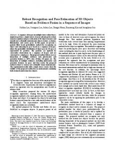
Fig. 1. (a) The image-template with the selected landmark points annotated around them, (b) and (c) the triangulation of the landmark points of both template landmark points and the current landmark point in the image. (d) The visualization of the weighted values of the template (See Section III-B).

(i) First a set of landmark points is marked around the image-template T as shown in Fig. 1. The locations of these landmark points can be represented by a shape vector: s = [u 1 v2 . . . um vm ], where (ui vi ) are the coordinates of the ith landmark point. Usually, the selection of these landmark points is manually specified in the learning phase. (ii) Then AAM employs a shape deformation function s(p) : RK → R2m that is a mapping from the K-dimensional parameter space to the 2m-dimensional space of landmark point locations. Intuitively, this function is used to project the template landmark points onto the current image I and to govern the movement (i.e. deformation) of these image landmark points by varying the parameter p. In other words, by specifying a fixed p  , this function provides an instance of landmark point positions  T ] in the image. s (p ) = [u1 v1 . . . um vm In AAM, this shape deformation function is derived from a set of training samples which consists of training images with human-marked landmark points. That is, from the landmark

points extracted from training images – given by the set of shape vectors ts 1 , ts2 , ts3 , . . . – a PCA-based procedure is applied to obtain the mean shape s 0 and the shape eigenvectors s1 s2 . . . sk . Then the shape deforming function can be modeled in terms of the shape parameters p = [p1 p2 . . . pk ] as: s (p) = s0 +

K


pj sj

(2)

j=1

(iii) Finally, the warping function that relates the template pixel location to the image pixel location can be parametrized in terms of the shape parameters p by using a piecewise affine warping [14] consisting of the following steps. First the landmark points in both the template and the current image are triangulated using, for example, Delaunay triangulation, as shown in Fig. 1(b) and 1(c). Usually, the information of these triangles is pre-computed, for obvious reasons, in the learning stage and used in subsequent images during the tracking stage. Next, an affine warping is applied to each pair

232

P. Mittrapiyanuruk and G.N. DeSouza / Tracking 3D pose of rigid objects using Inverse Compositional Active Appearance Models

Fig. 2. The affine warping between the pixels of a pair of triangles.

of corresponding triangles. That is, if we consider the ith pair of triangles shown in Fig. 2, which assumes that the vertices on the temT T T plate are [u1 v1 ] , [u2 v2 ] and [u3 v3 ] and the vertices on the current image are respecT T T tively [u1 v1 ] , [u2 v2 ] and [u3 v3 ] , then the warping function that relates a template pixel T location x = [u v] , lying inside this triangle to a corresponding image location W(x) can be expressed as in Eq. (3)   a u + a2 v + a3 W (x; a) = 1 (3) a4 u + a5 v + a6 T

where a = [a1 a2 . . . a6 ] is a set of affine warping parameters which can be computed from the coordiT T nates [u1 v1 ]T , [u2 v2 ]T , [u3 v3 ]T , [u1 v1 ] , [u2 v2 ] T and [u3 v3 ] (see [14] for more detail). Since the coT T T ordinates [u1 v1 ] , [u2 v2 ] and [u3 v3 ] are parametrically generated from the shape deforming function s(p) (see Eq. (2)), then the affine warping parameters of the ith pair of triangles can be expressed as the coefficients of the parameters p. i.e. a (i) (p) =  T (i) (i) (i) a1 (p) a2 (p) . . . a6 (p) . Note that each pair of triangles has its own affine warping parameters a (i) , but the parameters of all triangular pairs are functions of the global shape parameters p. The second key idea of AAM is that AAM models the variation of the object appearance (the variation of the template intensity) which can occur due to the illumination change, the deformation of the object, change in the object pose, etc. In AAM, this variation is handled by using the intensity-adjustable template. That is, instead of representing the object with a fixed image template T, AAM resorts to a parametrized template T(λ) which can adjust its intensity by varying the parameters λ. In AAM, this parametrized template

is computed in the way similar to the shape deforming function derivation. That is, from a set of imagetemplates warped into a reference frame and extracted from the training images obtained for various illuminations and object poses, a PCA based procedure is applied to obtain the mean template (T 0 ) and the eigenvectors (T1 , T2 , . . . Tl ) of the template intensity vectors. Then, the template can be parametrized in terms of the illumination parameters (λ) as in T (λ) = T0 +

l


λj Tj

(4)

j=1

Finally, with the implementation of a piecewise affine warping and the modeling of the appearance variation Eq. (4), the object localization problem in AAM can be recast as the image alignment problem (see Eq. (1)) for estimating the shape and the template intensity parameters through the minimization:

 p, λ = argmin T (x, λ) − i x∈Xi (5) 2   I W x; a(i) (p) where Xi is the set of template pixel locations lying T  (i) (i) (i) inside the ith triangle and a (i) = a1 a2 . . . a6 is the affine warping parameters of the i th triangle. The optimal parameters obtained from solving the above minimization will provide the identity, i.e. the 2D location of the landmark points of the object in the image I.

3. Method for tracking 3D pose of Rigid Objects using inverse compositional AAM In this section, first in Subsection 3.1, it is explained the idea of how to extend AAM for estimating the 3D

P. Mittrapiyanuruk and G.N. DeSouza / Tracking 3D pose of rigid objects using Inverse Compositional Active Appearance Models

pose of a rigid object. This idea is similar to the one in our previous work presented in [15]. Then, it is presented two major improvements over this previous works. The first improvement, presented in Subsection 3.2, is to incorporate the edge information of each template pixel in term of a weighted sum that represents the contribution of each pixel in the estimation. The second improvement, and the most important one, is presented in Subsection 3.3 and it consists of applying the inverse compositional algorithm to efficiently perform the minimization as in Eq. (5), where the formalization is now extended to the 3D case. 3.1. Extending AAM for estimating the 3D pose of rigid objects Since the focus in this work is on the 3D pose estimation of the object under rigid motion (3D translation and rotation), it is assumed that all possible movements of the object landmark points in an image can be generated from the perspective projection of the 3D coordinates of those landmark points under various 3D poses. Based on this assumption, it is more accurate to define the shape deformation function s(p) as in Eq. (2) with a function that involves the perspective projection of 3D model points. That is, if we define the 3D shape of the object by the 3D coordinates (w.r.t. an object coordinated frame) of the landmark points as ⎡ ⎤ X 1 . . . Xm ˆ = ⎣ Y1 . . . Ym ⎦ S (6) Z1 . . . Zm then, instead of using Eq. (2), the shape deformation function s(p) for the case of 3D pose estimation can also be expressed in terms of the 3D pose parameters p3d = [tx ty tz αx αy αz ] as:   u1 . . . un ˆ (7) s (p3d ) = = K ∗ H (p3d ) ∗ S v1 . . . vn Here, K is the camera’s constant intrinsic parameters, which are obtained from a camera calibration process, and H(p3d ) is a homogeneous transformation matrix representing the 3D pose parameters (p 3d ) of the object i.e.   R t (8) H (p3d ) = 000 1 where R = Rx (αx )Ry (αy )Rz (αz ), and Rx (αx ), Ry (αy ) and, Rz (αz ) are the rotation matrices representing the rotation about the x, y, z axes with the an-

233

gles αx , αy , αz respectively and t = [t x ty tz ]T is the translation along those same axes. By using the modified shape deformation function in Eq. (7), which is now a function of the 3D pose parameters (p3d ), we can apply the same derivation presented in Section 2. Then, we can obtain the same AAM image alignment minimization as in Eq. (5), but now with respect to the illumination parameters (λ) and the 3D pose parameters p 3d – i.e. the variable p in Eq. (5) is changed to p 3d . In summary, the 3D pose estimation problem has been recast as the problem of aligning the image-template T and the image I by adjusting the 3D pose parameters. In terms of other 3D approaches – i.e. [15,16] – the proposed method relies on a very sparse set of landmark points: roughly 30–100 landmark points. This number of landmarks is a few orders of magnitude smaller than the dense set of points used in [16] – more than 70,000 points in that case. Also, this set of 3D landmark points is obtained by applying a simple stereo vision technique. That is, we employ a pair of calibrated stereo-camera to acquire the images of the target object and use a simple tool that was developed in [15] to gather the landmark points. This software tool displays two stereo images of the object and guides the human in selecting landmark points in the left image and the corresponding point in the right image. After a few clicks of the mouse, and using simple 3D reconstruction, the 3D model of the object is created. Since this model is built carefully, practically by hand, it can be greatly more accurate than the one obtained using structure-from-motion, as in [18]. 3.2. Assigning the weight of each pixel in the image alignment The formulation in Eq. (5) assumes that every pixel provide an equal contribution to the image alignment minimization. However, if the texture (intensity pattern) of the template is too flat (i.e. there is not much information on the template pattern), an adverse effect can be induced on the minimization algorithm. Once again, this minimization algorithm is the one that searches for the warping parameters that minimize the intensity difference between template and current images. That is, while the algorithm performs the image alignment, the sum of the squares of the intensity difference of the flatted texture area, which covers the majority of the template, may predominate in the evaluation of the total error. This effect can reduce the ability by the algorithm of distinguishing any improve-

234

P. Mittrapiyanuruk and G.N. DeSouza / Tracking 3D pose of rigid objects using Inverse Compositional Active Appearance Models

ments in the error in each search direction and it can lead to an inaccurate image alignment or even to non convergence due to local minima. In order to alleviate this problem, we employ a weighted L2 formulation of the image alignment [2]. That is, instead of equally trusting every pixel in the image alignment, large weighted values are assigned to the pixels in the template area that have high gradient (i.e. edge structure). Similarly, small weights are assigned to the pixels in the texture-flat area (low gradient). Based on this idea, the problem can be further formulated as the following minimization:

q (x) . (p3D , λ) = argmin i x∈Xi (9)    2 (i) T (x; λ) − I W x; a (p3D ) where q(x) is the weight of the template pixel x and it can be computed from Eq. (10) as: |g(x)| q (x) = |g(x)| + |g0 |

minimization. Besides, the results show that if the template is represented with the edge structure above, then the gradient of this edge-template can never be so noisy as to degrade the accuracy of the method. That was exactly the reason not to approach this 3D pose problem as in Cootes’ work ([8]) – that is, directly align the edge template to the edge image. 3.3. Applying the inverse compositional algorithm As explained earlier, in order to perform the minimization step in Eq. (9) for object tracking, we propose the inverse compositional algorithm with a strategy of updating the pose parameters similar to [7]. That is, at each iteration, we assume that the current estimate of λ and p3d is known,1 then we solve for (∆p 3d , ∆λ) by minimizing   

 q (x) .T0 W x; a(i) (∆p3d ) + i

(10)

where |g(x)| is the magnitude of the gradient at the template pixel x, and |g 0 | is the mean of the magnitude of the gradient over all template pixels. The weights computed from the above equation for the template in Fig. 1 can be visualized as in Fig. 1(d) where the white area represents the pixels that have the weight closest to one. As pointed out in [17], Eq. (10) has the effect of limiting very large weights, and can keep the pixels from predominating in the image alignment process. Also the weights computed from this equation have the property that the pixels whose |g(x)| are less than |g0 | (noisy, approximately flat region) tend to get the smaller weight (closest to zero) and the pixels whose |g(x)| is above |g0 | (edge region) tend to get the larger weight (closest to one). In fact, the formula in 10 was originally proposed by Cootes et al. [8] for computing the edge structure from the raw intensity of the template. In that case, instead of representing the template with the pixel intensity, this edge structure was directly used for representing the template in the image alignment – i.e. the edge-template. However, unlike in their work, here we use a similar formulation to calculate the weight that controls the contribution of each pixel in the image alignment. As we will mention in the next section, the proposed inverse compositional algorithm requires the evaluation of the spatial gradient of the template i.e. ∇T, while it efficiently performs the image alignment

l


x∈Xi

(11)    (λk + ∆λk ) Ti (x) − I W x; a(i) (p3d )

k=1

and updating the parameters as in λ ← λ + ∆λ

(12) −1

H (p3d ) ← [H (∆p3d )]

∗ H (p3d )

(13)

These two steps – parameter calculation Eq. (11) and parameter updating Eqs (12) and (13)) – are iteratively executed until convergence of the algorithm. After applying Taylor expansion to Eq. (11), it becomes   

∂W ∂a q (x) . T0 (x) + ∇T0 ∆p3d ∂a ∂p3d i x∈Xi

+

l


(λk + ∆λk ) Tk (x)

(14)

k=1

2   −I W x; a(i) (p3d ) ∂a where the term ∇T0 ∂∂W a ∂ p3d is evaluated at each x with p3d = 0.

1 In this work, we assume that the initial 3D pose parameters for the first frame in the image sequence are known. Then the initial pose parameters for the subsequent frames are obtained from the tracking result of the previous frame. That is, we leave the problem of the first frame initialization as future work.

P. Mittrapiyanuruk and G.N. DeSouza / Tracking 3D pose of rigid objects using Inverse Compositional Active Appearance Models

For the affine warping, ∂∂W a can be calculated for each triangle using   ∂W u v 1 0 0 0 = (15) 0 0 0 u v 1 ∂a where (u,v) is the coordinate of the template pixel x Also, for each triangle, ∂∂pa3d is the 6 × 6 Jaco-

(i) bian matrix of  the warping parameters a (p3d ) = (i) (i) a1 . . . a6 with respect to the 3D pose parameT

ters p3d = [tx ty tz αx αy αz ] and evaluated at p 3d =

T 000000 . The solution (∆p3d , ∆λ) for Eq. (14) can be obtained by linear least square ([2]). That is:   −1 T  ∆p3d J Qr (16) = JT QJ ∆λ where J = [M T1 . . . Tl ]is a N × (6 + l) matrix (N is number of the template pixels). M is a N × 6 matrix consisting of the terms ∂a ∇T0 ∂∂W a ∂ p3d for each pixel x. Ti are the eigenvectors of the intensity template i = 1, . . ., l in Eq. (4) Q is a N × N diagonal matrix whose diagonal elements correspond to the weights q(x) of the pixels x. r is a N × 1 vector of the error associated to each pixel x and r (x) = T0 (x) + 

l
k=1

λk Tk (x)

  −I W x; a(i) (p3d )

(17)

Since, for any specific template T(λ), the matrices J and Q are constant for all iterations, these matrices and their products in Eq. (16) can be pre-computed as part of the learning phase. The pre-computations of J and Q are key to the proposed method and is the reason for the method to be more efficient than any other previously proposed approach. However, to solve the linear system in Eq. (16), it is often the case that the matrices be ill-conditioned, leading to an unstable solution, which can cause the whole tracking algorithm to fail. In order to solve this problem, we apply the LevenbergMarquardt method to solve the above least square system. That is, we propose a Levenberg-Marquardt version of the Inverse Compositional algorithm in which, at each iteration step, instead of solving Eq. (16), the parameters are updated by solving



235



−1 T  ∆p3d J Qr = JT QJ + δΣ ∆λ

(18)

where Σ is a (6 + l) × (6 + l) diagonal matrix where each element (i, i) is computed from the sum of the square of the elements in the ith column of J, and δ is a damping factor which is dynamically adjusted depending on whether the error is decreasing or increasing during iterations. In summary, our algorithm can be described as follows: Pre-computing stage: 1. Compute the spatial gradient of the mean template (∇T0 ) 2. Compute ∂∂pa3d at p3d = 0 for each triangular meshes ∂a 3. Compute the Jacobian ∇T 0 ∂∂W a ∂ p3d at every template pixel by using the values ∂∂pa3d of the corresponding triangle. 4. Compute JT Q,JT QJ, and Σ Pre-Iteration stage: 1. Initialize δ = 0.001 2. Compute the affine warping parameters a (i) (p3d ) of each triangle from the current pose parameters p3d . 3. Compute the error image r as in Eq. (17) and the summation of error e = r 2 Iteration stage:

 −1 T 1. Compute JT QJ + δΣ , [J Q]r 2. Compute the update of pose and illumination parameters (∆p3d , ∆λ) by solving Eq. (18) 3. Update the pose and illumination parameters by Eqs (12) and (13) 4. Compute the affine warping parameters a(i) (p3d ) of each triangle from the current pose parameters p 3d . 5. Compute the error image r as in Eq. (17) and the summation of error e ∗ = r2 6. If e∗ < e then δ ← δ/10; e = e∗ else δ ← δ ∗ 10; undo step 3–5 untilp3d  < ε

Basically, the iteration steps of the proposed method (step 1–6 of “Iteration stage”) are in some sense similar to the ones in our previous work [15]. However, since the minimization method in the previous work was based on the Gauss-Newton method, it turns out that the resulting matrix was dependent on the pose parameters p3d . As mentioned earlier, this is the ma-

236

P. Mittrapiyanuruk and G.N. DeSouza / Tracking 3D pose of rigid objects using Inverse Compositional Active Appearance Models

Fig. 3. Qualitative results of the tracking.

trix required to be re-evaluated at each iteration, which made the algorithm quite inefficient. In general, the method using the weighted L2 norm formulation gives an accurate result if the initial aligned position is closed to the actual aligned position. If this initialization is poor, the largely weighted template pixels at the beginning of the minimization become very distant from their corresponding image pixels, and applying the method using the weighted formulation can easily lead to problems with local minima. In practice, to alleviate this problem, we apply the above algorithm using two consecutive phases. In the first phase, we apply the algorithm with equal weights for all template pixels – i.e. q(x) = 1 for all x. Then, after obtaining an approximate result from this first phase – i.e. an approximate 3D pose and illumination parameters – we apply the algorithm with the weighed formulation as explained in Section 3.2 to obtain a more accurate tracking result – more correctly aligned in the edge structure area.

3.4. Results and discussion In order to evaluate our method, we collected experimental data using a pair of stereo cameras mounted onto the end-effector of an industrial robot. The end-effector moved on several arbitrary paths around the target object, which remained stationary. While the robot is moving, a sequence of images (640 × 480 pixels) of the target object was acquired. At the same time, the position of the end-effector (from the direct kinematics of robot) was recorded for each image taken. In this way, the exact relative pose of the object can be determined – the same pose that will be used as the ground truth, as explained in more details shortly. For this experiment, we used an engine cover, shown in Fig. 1 as the target object. Also, two different sequences were stored: each one with a different background. For testing with the first sequence, we constructed the appearance model from the training images selected from the second sequence and vice-versa. For

P. Mittrapiyanuruk and G.N. DeSouza / Tracking 3D pose of rigid objects using Inverse Compositional Active Appearance Models

237

Table 1 Error in pose estimation for two test sequences. Here, we compare the proposed method, our previous method [15], and the geometric-based method in [19] Statistics of the Error in Pose Estimation SEQ #1 Proposed Method Avg Std Max Previous Method [15] Avg Std Max Geometric Method [19] Avg Std Max SEQ #2 Proposed Method Avg Std Max Previous Method Avg Std Max Geometric Method Avg Std Max

x-trans (mm) 6.3 5.5 26.5 6.9 5.6 25.2 11.2 9.1 48.8 6.2 5.5 25.5 5.5 5.9 23.6 14.9 11.1 52.1

y-trans (mm) 5.2 5.7 23.1 5.4 5.8 23.1 8.1 7.1 37.2 5.5 5.6 21.0 5.5 5.9 22.1 7.9 6.4 29.2

the training images in both tests, we selected 16 images from different viewpoints, and each training image was annotated with 76 landmark points, as shown in Fig. 1. To construct the 3D model of the target object, we select a second image from a stereo pair acquired from the frontal view position. The qualitative results for the proposed method using both sequences can be observed in Fig. 3. As this figure shows, the estimated pose – represented by the yellow-dotted line superimposed onto the image – always matches the actual border of the area defined by the exterior landmark points as well as the interior landmark points. The tracking results were good for all poses of the objects, independently of the backgrounds. In order to extract quantitative results,we determined the accuracy of our method by comparing the estimated pose of the end-effector with the same pose obtained using the robot kinematics (ground truth). This relative pose, or motion, of the end-effector is expressed in homogeneous transformation by ei He0 and it represents the end-effector’s position e i at the time we acquired the ith image with respect to an arbitrary reference position e0 of the end-effector. Since the object is stationary with respect to the base of the robot, this relative motion of the end-effector can be perceived instead as the relative motion of the object with respect to the end-effector (or the camera mounted on it). As mentioned earlier, we recorded the end-effector position, which basically is the transformation ei Hb with respect to the robot base, at each time we acquired an image. From these data, the ground truth at each frame can be easily obtained by:

z-trans (mm) 2.9 3.1 13.4 2.9 3.1 13.5 3.4 3.7 31.8 3.5 3.5 17.2 3.6 3.4 16.5 4.2 4.5 23.0

x-rot (deg) 0.33 0.31 1.27 0.34 0.31 1.17 0.51 0.43 2.26 0.34 0.32 1.41 0.34 0.32 1.27 0.48 0.39 1.64

y-rot (deg) 0.37 0.43 1.71 0.40 0.43 1.66 0.76 0.55 3.06 0.47 0.38 1.88 0.45 0.39 1.74 0.96 0.80 3.77

z-rot (deg) 0.14 0.12 0.49 0.14 0.13 0.51 0.27 0.22 1.04 0.12 0.13 0.57 0.14 0.13 0.52 0.23 0.18 1.00

(ei He0 )groundtruth =ei Hb ∗ (e0 Hb )−1

(19)

Meanwhile, using the estimated pose from our method, we calculated the same transformation by (ei He0 )estimate =e Hc ∗ci Ho ∗ [e Hc ∗c0 Ho ]−1 (20) where e Hc is a constant hand-to-eye transformation matrix obtained during the camera calibration process [12], ci Ho is the estimated object pose with respect to the camera (mounted onto the end-effector) at the time of frame i – which was obtained from our method – and c0 Ho is the object pose with respect to the camera at the reference (initial) position of the end-effector – which was also obtained by applying the method to the image at time of frame 0. Next, we compared the accuracy of our new method with the accuracy of our previous method [15] and with the accuracy of a previously developed algorithm using geometric features [19]. The algorithm using geometric features was already very accurate in terms of its application in industrial automation, which makes it a good reference for comparison with this new method. In Fig. 4, we depict the accuracy measurements by plotting (ei He0 ) in terms of their translational and rotational components. The same figure shows the 3D poses obtained using: the ground truth; the proposed method; our previous method; and a geometric-based method. Also, the statistics of the error between the estimated and the actual pose for each of the 6 degree of freedom over the whole test sequence are summarized in Table 1. As it can be inferred from Table 1 and the curves in Fig. 4, the accuracy of both of our methods – the

238

P. Mittrapiyanuruk and G.N. DeSouza / Tracking 3D pose of rigid objects using Inverse Compositional Active Appearance Models

Fig. 4. Plotting of translational and rotational coefficients of eiHe 0 using: the ground truth; our new method; our previous approach [15]; and the geometric approach in [19].

newly proposed one and the previous one – are somehow equivalent. This observation validates the modifications implemented in this new method as a form of speedup that does not compromise the accuracy. Also, in the same table, we observe an average error for all translational components always smaller than 0.65 cm. with a very small standard deviation: usually less than 0.6 cm. In terms of rotational error, the error is in average only 0.45 degree, with also very small standard deviations: less than 0.4 degree. Also, our new method has proved to be superior to the method using geometric features, especially if we consider the large peaks present in the latter method. Furthermore, the stability of the estimation of this new method is also better than the geometric-based approach. This fact can be observed in the graphs of Fig. 4 by the high frequency noise on top of the curve

for the geometric-based method. This noisy estimation can be more harmful in the context of a visual servoing system because it may cause the end-effector to move jerkily. In terms of the processing time, the speed of the new method for object tracking is dependent on many factors, as for example, the number of template pixels, the initial pose, the object model, etc. Currently, we implemented the proposed method using MATLAB and the average speed of the algorithm running on a Pentium IV 3.9 GHz is about 5.1 seconds per frame, where the size of the template is about 72,000 pixels and the initial pose of each frame is randomly perturbed around the actual pose. In comparison to our previous method, which was implemented using Visual C++ on the same computer, the average speed was about 12 seconds per frame. That represents an enormous im-

P. Mittrapiyanuruk and G.N. DeSouza / Tracking 3D pose of rigid objects using Inverse Compositional Active Appearance Models

provement, since the new method is already faster even running using MATLAB. Usually, a C implementation of any algorithm is at least 10 times faster than its MATLAB implementation. But we believe that this speed can be increased even further by using a multi-resolution (coarse-to-fine) technique, which would also prove to be beneficial in term of the robustness of the algorithm.

[2] [3]

[4]

[5]

[6]

4. Conclusion and future work We presented an efficient and accurate method to track rigid objects using a modified version of Active Appearance Model (AAM) and the inverse compositional image alignment algorithm. We demonstrated the accuracy of our method against the ground truth, as well as a early developed method using geometric features [19]. Finally, we also compared our method to a not-so-efficient, but very accurate method derived from our previous work [15]. The result showed that our new method worked as accurately as our previous works – only a few millimeters of error. The results also showed that the new method outperformed the geometric-based method. The proposed method presents one drawback: it requires the initialization of the parameters regarding the object pose at the beginning of the iteration for a successful tracking of future image frames. Currently we have to manually provide a rough initial estimate of such pose parameters for the very first frame. Since our goal in the future is to apply this method for automation using visual servoing, we must substitute this initialization with some automatic estimate of the first pose.

[7]

[8] [9]

[10]

[11]

[12]

[13]

[14]

[15]

Acknowledgment

[16]

The authors would like to thank Dr. Dana Cobzas for many insightful discussions of her algorithm.

[17]

References

[18]

[1]

J. Ahlberg, Using the active appearance algorithm for face and facial feature tracking, In IEEE ICCV Workshop on Recognition, Analysis, and Tracking of Faces and Gestures in RealTime Systems, 2001, pp. 68–72.

[19]

239

S. Baker, R. Gross, I. Matthews and T. Ishikawa, Lucas-kanade 20 years on: A unifying framework: Part 2. Technical report. S. Baker and I. Matthews, Lucas-kanade 20 years on: A unifying framework, International Journal of Computer Vision 56 (2004), 221–255. V. Blanz and T. Vetter, Face recognition based on fitting a 3d morphable model, IEEE Trans PAMI 25 (Sep 2003), 1063– 1074. J.M. Buenaposada and L. Baumela, Real-time tracking and estimation of plane pose. In Proceedings of the IEEE ICPR, (vol. 2), Aug 2002, pp. 697–700. M.L. Cascia, S. Sclaroff and V. Athitsos, Fast, reliable head tracking under varying illumination: An approach based on registration of texture-mapped 3d models, In IEEE Transactions on Pattern Analysis and Machine Intelligence 22 (2000), 322–336. D. Cobzas and M. Jagersand, 3d ssd tracking from uncalibrated video. In Workshop in Spatial Coherency for Motion, ECCV, 2004. T.F. Cootes and C.J. Taylor, On representing edge structure for model matching. In Proceedings of CVPR. T.F. Cootes, G.J. Edwards and C.J. Taylor, Active appearance models. In 5th European Conference on Computer Vision, (vol. 2), 1998, pp. 484–498. F. Dellaert, C. Thorpe and S. Thrun, Super-resolved texture tracking of planar surface patches. In Proceedings of the IEEE/RSJ IROS, (vol. 1), 1998, pp. 197–203. D. Gennery, Visual tracking of known three-dimensional objects, International Journal Computer Vision 7 (1992), 243– 270. R. Hirsh, G.N. DeSouza and A.C. Kak, An iterative approach to the hand-eye and base-world calibration problem. In Proceedings of 2001 IEEE International Conference on Robotics and Automation, (vol. 1), Seoul, Korea, May 2001, pp. 2171– 2176. B. Lucas and T. Kanade, An iterative image registration technique with an application to stereo vision. in Proceedings of International Joint Conference on Artificial Intelligence, 1981, pp. 674–679. I. Matthews and S. Baker, Active appearance models revisited, International Journal of Computer Vision 60(2) (2004), 135– 164. P. Mittrapiyanuruk, G.N. DeSouza and A.C. Kak, Calculating the 3d-pose of rigid objects using active appearance models. In Proceedings of 2004 IEEE International Conference on Robotics and Automation, New Orleans, USA, April 2004, pp. 5147–5152. S. Romdhani and T. Vetter, Efficient, robust and accurate fitting of a 3d morphable model. In Proceedings of the 9th IEEEICCV, 2003, pp. 59–66. I.M. Scott, T.F. Cootes and C.J. Taylor, Improving appearance model matching using local image structure. In Proceedings of Information Processing in Medical Imaging, 2003, pp. 258– 269. J. Xiao, S. Baker, I. Matthews and T. Kanade, Real-time combined 2d+3d active appearance models, In Proceedings of the IEEE Conf. on CVPR, June 2004. Y. Yoon, G.N. DeSouza and A.C. Kak, Real-time tracking and pose estimation for industrial objects using geometric features. In Proceedings of 2003 IEEE International Conference on Robotics and Automation, Taiwan, May 2003, pp. 3473–3478.