Tracking of the expected time to reinforcement in temporal ...

Learning & Behavior 2003, 31 (1), 3-21

Tracking of the expected time to reinforcement in temporal conditioning procedures KIMBERLY KIRKPATRICK University of York, York, England and RUSSELL M. CHURCH Brown University, Providence, Rhode Island In one experiment, the rate and pattern of responding (head entry into the food cup) under different distributions of intervals between food deliveries were examined. Separate groups of rats received fixed-time (45, 90, 180, or 360 sec), random-time (45, 90, 180, or 360 sec), or tandem fixed-time (45 or 90 sec) random-time (45 or 90 sec) schedules of reinforcement. Schedule type affected the pattern of responding as a function of time, whereas mean interval duration affected the mean rate of responding. Responses occurred in bouts with characteristics that were invariant across conditions. Packet theory, which assumes that the momentary probability of bout occurrence is negatively related to the conditional expected time remaining until the next reinforcer, accurately predicted global and local measures of responding. The success of the model advances the prediction of multiple measures of responding across different types of time-based schedules.

The focus of empirical and theoretical developments in the f ield of animal timing has been on the analysis of fixed-interval performance. If a rat is presented with a light for 30 sec, after which pressing a lever will result in food delivery, the rat will demonstrate an increasing rate of leverpressing as a function of time since light onset. This response pattern indicates that the rat has learned the duration of the light. Timing theories, such as scalar timing theory (Gibbon & Church, 1984; Gibbon, Church, & Meck, 1984), multiple oscillator model (Church & Broadbent, 1990), behavioral theory of timing (Killeen & Fetterman, 1988), and the learning to time model (Machado, 1997), accurately predict fixed-interval timing. In the natural environment, events rarely occur at precise periodic intervals. The focus on fixed intervals may fail to disclose important features of the timing system, because it has evolved under conditions of temporal uncertainty. In a few studies, variable-interval performance has been examined, and these studies have indicated that exponential random intervals result in a relatively constant rate of responding as a function of time (Catania & Reynolds,

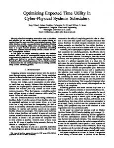
1968; Church & Lacourse, 2001; Kirkpatrick & Church, 2000b; LaBarbera & Church, 1974; Libby & Church, 1975; Lund, 1976), in contrast to the increasing response rate observed with fixed intervals. Various proposals have been made in an attempt to explain the pattern of responding under fixed and random intervals. The goal is to account for the pattern of responses as a function of the pattern of delivery of reinforcers. The top row of functions in Figure 1 are the density functions for three reinforcement schedules: fixed time (FT) 90, in which food is delivered every 90 sec; random-time (RT) 90, in which food is delivered at exponentially distributed intervals with a mean of 90 sec; and FT75–RT15, in which food is delivered after 75 sec plus an exponentially distributed interval with a mean of 15 sec. Alternative representations of these three density functions include the survival function, the hazard function, and the conditional expected time function (shown in rows 2–4 of Figure 1). Appendix A provides the definitions of these functions. Scalar timing theory (Gibbon & Church, 1984; Gibbon et al., 1984) assumes that responding in a fixed-interval schedule is based on a random sample of the remembered times of reinforcement but that responding in a variableinterval schedule is initiated by a random sample of the shortest remembered times of reinforcement and is terminated by a random sample of the longest remembered times of reinforcement (Brunner, Fairhurst, Stolovitzky, & Gibbon, 1997; Brunner, Kacelnik, & Gibbon, 1996). An alternative approach is to assume that responding under fixed intervals is based on the density function with added sources of variance but that responding under random intervals is controlled by the hazard function, which reflects the conditional probability of receiving food,

National Institute of Mental Health Grant MH44234 to Brown University supported this research. National Research Service Award MH11691 from the National Institute of Mental Health supported K. K. Special thanks are extended to An Le for his assistance in formulating the explicit solution of the conditional expected time function. The raw data (time of occurrence of each response and reinforcer on each session for each rat) are available at http://www.Brown.edu/Research/Timelab. Correspondence concerning this article should be addressed to K. Kirkpatrick, Department of Psychology, University of York, York YO10 5DD, England (e-mail: [email protected]). —Accepted by previous editorial team of Ralph R. Miller.

3

Copyright 2003 Psychonomic Society, Inc.

4

KIRKPATRICK AND CHURCH

Figure 1. The density, survival, hazard, and conditional expected time functions for a fixed-time (FT) 90-sec, a random-time (RT) 90-sec, or a tandem FT75–RT15-sec interval. The horizontal axis of each panel of the figure is the time since an event, such as stimulus onset or food delivery.

given that food, has not yet occurred (Catania & Reynolds, 1968). (See Anger, 1956, for the application of the hazard function to interresponse time [IRT] distributions in DRL schedules.) As is shown in Figure 1, the hazard function for a random interval is constant over time and, therefore, could explain the relatively constant rate of responding that is observed. However, a different distribution form is required for fixed-interval performance, because the hazard function does not map onto response rate. One could use the hazard function with added variability to explain both fixed- and random-interval performance, but this would lead to a departure from constancy in the random-interval case and, therefore, would not accurately fit the data.

A third proposal has been to assume that temporal control over behavior decreases as variability increases, so that fixed intervals exhibit strong control but (exponential) random intervals exhibit no control over behavior (Lund, 1976). All three approaches propose different processes in random and fixed intervals. This leads to the unparsimonious conclusion that there may be multiple timing systems, each tuned to a different distribution form. A simpler alternative would be to assume that temporal performance is controlled by some common aspect of different distribution forms. In addition to an examination of the effects of variability on responding, the present experiment provided an as-

EXPECTED TIME TO REINFORCEMENT sessment of the role of mean interval duration. Interval duration usually is negatively related to measures of response rate or strength (Bitterman, 1964; Black, 1963; de Villiers & Herrnstein, 1976; Gibbon, Baldock, Locurto, Gold, & Terrace, 1977; Herrnstein, 1970; Salafia, Terry, & Daston, 1975; Schneiderman & Gormezano, 1964). This relationship is often reported to be nonlinear in form (e.g., Herrnstein, 1970). Predictions of the rate of responding have traditionally required a separate explanation from predictions of the pattern of responding in interval-based procedures. For example, Herrnstein’s hyperbolic rule (de Villiers & Herrnstein, 1976; Herrnstein, 1970) predicts that the absolute rate of responding is a nonlinear function of the rate of reinforcement (the reciprocal of interval duration). Herrnstein’s rule provides a good quantitative fit to mean response rate data obtained under both fixed- and random-interval schedules of reinforcement (Davison & McCarthy, 1988), but it does not make any predictions about the timing of responding during the interval. The main goal of the present paper is to integrate the effects of interval distribution form and mean interval duration with a theoretical framework that also predicts fixed-interval performance. It has been proposed that the conditional expected time function could predict responding under both fixed- and random-interval distributions (Kirkpatrick & Church, 2000b). Rats were trained with FT 90-sec, RT 90-sec, or tandem FT75–RT15-sec schedules of food delivery. (In this tandem schedule, food was delivered after 75 sec plus a random time with a mean of 15 sec.) The form of the response rate function was negatively related to the form of the conditional expected time function (bottom of Figure 1): linearly increasing rates of responding for FT, relatively constant response rates for RT, and increasing response rates during the FT portion and relatively constant response rates during the RT portion of the tandem schedule. The conditional expected time function, shown in the bottom row of Figure 1, is the mean expected time until the next food delivery at t sec after an event. The conditional expected time function is given in Equation 1, where f(x) is the density function of the variate x (Figure 1, top row) and S t is the survival function at time t (Figure 1, second row). The density function, f (x), is the probability density of food delivery at x sec after an event. The survival function, St, is the probability that food will not have occurred by time t in the interval: Et =

¥

é x f (x) dx - t . ê S t x=t ë

ò

(1)

For simple density functions, such as the ones used in the present experiment, the conditional expected time function can be calculated explicitly (see Appendix A), and for any empirical probability density function, the conditional expected time function can be obtained by numerical integration with the duration of the units (dx) set at some short interval. The expected time functions may also predict the effect of interval duration on the mean rate of responding. The

5

mean interval duration is equal to the expected time at interval onset. In Figure 1, the expected time to food immediately after an event (such as food or stimulus onset) is 90 sec for the FT90, RT90, and FT75–RT15 intervals. Thus, the mean rate of responding on all three of these distribution types should be the same, even though the pattern of responding should be different. The present experiment attempted to expand on the findings of Kirkpatrick and Church (2000b) by delivering four interval durations from each of three distribution forms: fixed, random, and tandem. The experiment assessed the generality of the expected time function in predicting response rate and form across a range of interval durations and distribution forms. If successful, a singleprocess account could serve to unify a large set of empirical phenomena in both classical and operant conditioning. METHOD Subjects Sixty male Sprague Dawley rats (Taconic Laboratories, Germantown, NY) were housed individually in a colony room on a 12:12-h light:dark cycle (lights off at 8:45 a.m.). Dim red lights provided illumination in the colony room and the testing room during the dark phase. The rats were fed a daily ration that consisted of 45-mg Noyes pellets (Improved Formula A) that were delivered during the experimental session and an additional 15 g of FormuLab 5008 food given in the home cage shortly after the daily sessions. Water was available ad lib in both the home cages and the experimental chambers. The rats arrived in the colony at 49 days of age and began training when they were 67 days old. Apparatus Each of the 12 chambers (25 3 30 3 30 cm) was located inside of a ventilated, noise-attenuating box (74 3 38 3 60 cm). A chamber was equipped with a food cup and a water bottle. A magazine pellet dispenser (Model ENV-203) delivered 45-mg Noyes (Improved Formula A) pellets into the food cup. Each head entry into the food cup was transduced by an LED photocell. The water bottle was mounted outside the chamber; water was available through a tube that protruded through a hole in the back wall of the chamber. Two Gateway 486 DX2/66 computers running the Med-PC Medstate Notation Version 2.0 (Tatham & Zurn, 1989), controlled experimental events and recorded the time at which events occurred with 10-msec resolution. Procedure The rats received single food pellets on FT, RT, or tandem FT–RT schedules. The pellets were delivered regardless of any behavior of the rats. There were four FT schedules of FT45, FT90, FT180, and FT360 sec, four RT schedules of RT45, RT90, RT180, and RT360 sec, and four tandem schedules of FT45–RT45, FT45–RT90, FT90–RT45, and FT90–RT90 sec. For the FT groups, food was delivered at regular intervals. For the RT groups, the food–food interval was an exponential distribution with an appropriate mean, which is a standard and eff icient way of generating random variables 1 (Evans, Hastings, & Peacock, 1993). For the FT–RT groups, food was delivered after a fixed duration plus an exponential random duration. For example, in the FT45–RT45 condition, once food was delivered, the next food could not occur for at least 45 sec and would occur, on average, after 90 sec. There were no external cues to signal the fixed or random portions of the food–food interval. These intervals are expressed as an FT followed by a random waiting time, because psychologically, the fixed minimum delay would seem to occur first. However, the schedule could be expressed as a random

6

KIRKPATRICK AND CHURCH iazakis (1999). First, a distribution of log IRTs was obtained (Figure 2). If responses occur in bouts, this distribution should be bimodal. Second, the bimodal IRT distribution was fit with a double-Gaussian (Equation 2), where p is the probability that an interresponse time falls in the first distribution, m1 is the mean of the first distribution, s1 is the standard deviation of the first distribution, m2 is the mean of the second distribution, and s2 is the standard deviation of the second distribution. The parameter settings that yielded the best fit with an v2 of .98 were p 5 .78, m1 5 0.17, s1 5 0.71, m2 5 1.66, and s2 5 0.38. The means in seconds were m1 5 1.50 sec and m2 5 45.86 sec. The two underlying single distributions were determined from the parameter settings. The cross point of the two distributions is the optimal criterion that minimizes the probability of misclassifying IRTs.2 For the data in Figure 2, the optimal criterion was 17.8 sec, and the probability of misclassification was .07. Some misclassification is unavoidable because the distributions overlap. yt = p

Figure 2. Bimodal distribution of interresponse times in equal 0.05-sec log10 time intervals. The heavy line is the best-fitting doubleGaussian function. The dashed lines are the underlying singleGaussian functions. The point where the two single-Gaussian functions cross (17.8 sec) is the optimal interresponse time criterion for determining the boundaries between bouts.

duration followed by a fixed duration, because the sum of two variables is the same regardless of order. The rats were randomly assigned to the fixed, random, and tandem conditions. There were a total of 6 rats per group in the fixed and random conditions and 3 rats per group in the tandem conditions. Each session lasted for 2 h, and each group was trained until approximately 320 reinforcements had been received. This required 2, 4, 6, 8, and 16 sessions for groups that received mean interval durations of 45, 90, 135, 180, and 360 sec, respectively. Data Analysis The time of occurrence of each head entry into the food cup (each time the photobeam was interrupted) and the time of each food delivery were recorded with 10-msec accuracy. Several measures of performance were calculated over the last half of training. Local response rate. Local response rates were determined over the food–food interval by calculating the number of responses (N t ) and the number of seconds of opportunity to response (Ot ) in each 5-sec bin following food delivery. When the intervals were fixed, the number of seconds of opportunity to respond in each 5-sec interval was equal to the total number of food–food intervals included in the analysis; when the intervals contained a random component, the number of seconds of opportunity to respond differed from bin to bin. Local rate, expressed as responses per minute, was then defined in each bin as 60*Nt /Ot . Bout analyses. A bout should include responses that are sufficiently close to constitute a run of responding, but should not include longer pauses that indicate a break in responding. Figure 2 contains the distribution of IRTs across all the rats, plotted in logarithmically spaced bins. The distribution of IRTs was bimodal, with one mode of about 1 sec, a trough of about 10–20 sec, and a second mode of about 50 sec. The mode of short IRTs primarily contains pauses in responding during a bout, and the mode of long IRTs contains pauses between bouts. The optimal criterion for defining bouts would lie between the two modes, because it would include the short IRTs within the bout but would exclude longer pauses between bouts. The optimal criterion was determined using a method proposed by Tolkamp and Kyr-

æ - (t - m1 ) 2 ö 1 exp ç ÷ è 2s 12 ø s 1 2p

æ - (t - m 2 )2 ö (2) exp ç ÷. è s 2 2p 2s 22 ø Within each food–food interval, the start of a bout was identified when the IRT between two consecutive responses was less than or equal to 17.8 sec; the first response in the pair was tagged as the start of a bout. The end of a bout was identified as the last response before a pause in responding of 17.8 sec or longer. Any number of bouts could be identified in a food–food interval, but a bout could not continue beyond the time that food was delivered. Responses rarely occurred outside of bouts. Across all of the groups, the response rate between bouts was 0.3 responses/ min. Several summary measures of the bouts were calculated: (1) the number of responses in a bout, (2) bout duration, (3) the response rate in a bout in responses per minute, and (4) the IRT in a bout. In addition, analyses were conducted on the pauses between bouts, defined as the time from the end of one bout until the start of the next bout in a food–food interval; this analysis required at least two bouts in an interval. Probability of being in a bout. Using the start and end times for each bout, a calculation was made of the probability of being in a bout during each second of the food–food interval. Each 5-sec bin during which the rat produced a bout was filled with a 1. If a bout started at 34.8 sec and ended at 41.2 sec, the 5-sec bins starting with 30 sec and ending with 45 sec would be filled. The probability of being in a bout was then the total number of 1s in each bin, divided by the total number of food–food intervals. + (1 - p )

1

RESULTS Local Response Rates The local rate of responding was examined for each group to determine the effect of interval duration and distribution form on the rate and pattern of responding in time. Figure 3 displays the response rate functions for the groups that received fixed (top panel), random (middle panel), or tandem (bottom panel) durations between successive food deliveries. All of the groups produced an initial high rate of responding, probably owing to consumption of the previous food pellet. Following that, there were noticeable differences in the response rate functions. The groups that received fixed intervals produced increasing response rate functions, the groups that received random intervals produced relatively constant response rate func-

EXPECTED TIME TO REINFORCEMENT

7

in Figure 4, plotted on double-log coordinates, with different distribution forms marked by different symbols. A mean response rate was calculated for each rat, beginning at 21 sec after food delivery and continuing until the next food delivery; the first 20 sec were removed because the consumption of the food resulted in a temporary increase in responding that was unrelated to the anticipatory response. The points in Figure 4 are the means for the rats in each group. The mean rates fell along a single straightline fit, with a slope of 20.98 and an intercept of 2.66; all of the data points fell within the 95% confidence interval band (dashed lines). A regression analysis was conducted on the log response rates, with the factors of log interval duration and distribution form, with factors entered simultaneously. The overall regression model was significant [F(2,9) 5 12.9, p , .01]. Log interval duration was a predictor of log response rate [t(4) 5 25.1, p , .01], but distribution form was not [t(2) 5 20.5]. Response Bouts The local response rate curves in Figure 3 were composed of many individual bouts. Figure 5 displays distributions of four measures of the response bouts: the number of responses per bout (top left panel), bout duration (bottom left panel), the IRTs in a bout3 (top right panel), and the response rate in a bout (bottom right panel). Each panel of the figure contains separate curves for the groups that received fixed, random, or tandem schedules. The curves are averaged across interval duration, which had no effect on the shape of the curves. The means of each measure are presented in Table 1 for individual groups. One striking feature of Figure 5 (and Table 1) is that interval

Figure 3. Effects of interval distribution form and mean interval duration on the response rate in responses/minute as a function of time since food for the fixed, random, and tandem conditions.

tions, and the groups that received tandem intervals produced response rate functions that contained an increasing portion followed by a relatively constant portion. Overall Response Rates Shorter intervals resulted in higher response rates than did longer intervals. This effect is displayed more clearly

Figure 4. Mean response rate is negatively related to mean interval duration: The mean response rate in log 10 responses/minute as a function of mean interval duration in log 10 seconds. Each data point is the mean of all the rats that received a particular condition of training. The solid line through the data points is the best-fitting straight-line regression, and the dashed lines show the 95% confidence intervals.

8


Figure 5. Invariance in the bout characteristics. The curves for the fixed, random, and tandem conditions are the means across all the rats that received a particular interval distribution form. Top left panel: the probability distribution of the number of responses per bout. Top right panel: the probability distribution of interresponse times during a bout in successive 0.1-sec intervals. Bottom left panel: the probability distribution of bout durations in successive 1-sec intervals. Bottom right panel: the probability distribution of response rates in responses/minute during a bout.

distribution form and interval duration had no effect on the characteristics of the response bouts. This was confirmed by an analysis of variance (ANOVA) conducted on the mean number of responses, bout duration, response rate, and IRTs (see Table 1), which revealed no effect of interval duration [all Fs(4,49) , 1] or distribution form [all Fs(2,49) , 1] and no interaction [all Fs(4,49) , 1]. The probability decreased geometrically as a function of the number of responses in a bout, with a minimum of 2 responses (see the Data Analysis section) and a mean of 5.7 responses (see Table 1). The probability decreased exponentially as a function of bout duration, with a mean of 12.7 sec. The probability decreased exponentially as a function of IRT, with a mean of 3.0 sec. The probability increased as a function of the response rate (in responses/ minute) up to approximately 15 responses/min and then decreased exponentially; the median response rate was 40.8 responses/min. A median was used instead of a mean because there were occasionally very large outliers at the tail of the distribution of response rates. This was typically

caused by bouts that contained two responses very close together in time. Although the overall distribution of IRTs was approximately exponentially distributed, it is possible that successive IRTs were not randomly distributed. For example, there may have been a tendency to engage in short–long oscillations in the time between responses, or the IRT may have decreased or increased over the course of the bout. For each response bout containing at least four responses, an autocorrelation was calculated on the IRTs. A second autocorrelation was calculated on a random ordering of the IRTs in each bout.4 If a pattern was present in the IRTs, the autocorrelation of the actual ordering of the IRTs would be different from the autocorrelation of the random ordering. For each rat, the mean autocorrelation across packets containing at least four responses was determined; these means were entered into an ANOVA. There was no difference in the autocorrelation between original (r 5 2.22) and random (r 5 2.22) ordering of the IRTs [F(1,49) , 1].

EXPECTED TIME TO REINFORCEMENT DISCUSSIO N

Table 1 Bout Characteristics for Each of the Fixed, Random, and Tandem Interval Groups Group FT45 FT90 FT180 FT360 RT45 RT90 RT180 RT360 FT45–RT45 FT45–RT90 FT90–RT45 FT90–RT90 Mean

Mean No. of Mean Bout Response Rate Mean Responses Duration (sec) (responses/min) IRT 6.4 5.5 5.4 4.8 6.4 8.0 5.3 5.0 9.4 4.5 3.7 4.1 5.7

14.0 11.9 14.9 10.4 16.1 14.4 11.3 11.9 19.3 12.1 6.6 9.6 12.7

34.8 41.3 37.8 40.0 35.3 43.3 40.6 32.9 40.1 37.7 66.2 39.0 40.8

9

2.8 2.7 3.6 2.6 3.0 2.5 3.0 3.0 2.3 3.7 2.9 3.3 3.0

The Temporal Structure of Bouts The present experiment identified two forms of temporal structure in the behavior of rats on temporal conditioning procedures. First, the response rate functions were composed of bouts that were unaffected by interval duration or distribution form (Figure 5 and Table 1). The bout characteristics were consistent with a random generating process, containing approximately six responses emitted

Note—The distributions of number of responses, bout duration, and interresponse time (IRT) were approximately exponential. In an exponential distribution, about two thirds of the samples will fall below the mean (Evans, Hastings, & Peacock, 1993).

There was also no effect of interval duration [F(4,49) 5 1.3] or distribution form [F(2,49) , 1] and no interaction [F(4,49) 5 1.3] on the original autocorrelations. Time Between Bouts Although the response bouts were unaffected by interval duration or distribution form, both variables affected the form and rate of responding. Therefore, the different conditions of training must have differentially affected the momentary rate of bout production. Figure 6 contains the probability distribution of pauses between bouts for the different conditions. The distribution of pauses fell more gradually as interval duration was increased. The probability of observing long pauses increased with interval duration, and the probability of observing short pauses decreased. The mean duration between bouts increased as a function of interval duration from around 22 sec in the 45sec conditions to around 110 sec in the 360 sec conditions. One-way ANOVAs conducted on the mean time between bouts revealed a significant effect of interval duration [F(4,49) 5 140.0, p , .001], but no effect of distribution form [F(2,49) 5 1.8] and no interval duration 3 distribution form interaction [F(4,49) , 1]. Probability of Being in a Bout A second measure that would reflect differences in the momentary probability of bout occurrence is the probability of being in a bout as a function of time in the interval (see the Data Analysis section). This is shown in Figure 7 for the fixed, random, and tandem groups of rats. The shape of these functions is essentially the same as the shape of the response rate functions. Following the initial reaction to food delivery, the fixed groups produced linearly increasing functions, the random groups produced constant functions, and the tandem groups produced linearly increasing functions followed by constant functions. Moreover, shorter interval durations resulted in a higher probability of being in a bout.

Figure 6. Probability distribution of pauses between bouts for fixed (top panel), random (middle panel), and tandem (bottom panel) intervals of different mean durations.

10


with an average IRT of about 3 sec. The distributions of the number of responses in a bout, bout duration, and IRT in a bout were approximately exponential in form, and there were no sequential dependencies between the IRTs of successive response pairs. This suggests that the structure of the bouts is unpredictable. The observation of bouts of behavior was made by Skinner (1938), who found that bursting of responses was independent of schedule type and attributed it to some characteristic inherent in the organisms themselves (p. 125). Subsequently, the bout-like nature of many operant and respondent behaviors, such as leverpresses, keypecks, orienting responses, magazine behavior, and drinking, has come to be well accepted (e.g., Blough, 1963; Corbit & Luschei, 1969; Fagen & Young, 1978; Gilbert, 1958; Mellgren & Elsmore, 1991; Nevin & Baum, 1980; Pear & Rector, 1979; Robinson, Blumberg, Lane, & Kreber, 2000; Schneider, 1969; Shull, Gaynor, & Grimes, 2001; Skinner, 1938; Slater & Lester, 1982). Because bouts of behavior are composed of short IRTs, prior findings that short IRTs are relatively insensitive to experimental manipulations, as compared with longer IRTs (Blough, 1963; Schaub, 1967; Shull & Brownstein, 1970), are consistent with the present findings regarding the invariance of bouts. The present analysis expands on earlier observations by demonstrating that many characteristics of bouts are invariant across a range of interval durations and distribution forms. Organization of Bouts When rats were trained with fixed, random, and tandem intervals of different durations between successive food deliveries, the local response rate as a function of time since food was affected by the distribution of intervals. On fixed intervals, response rates increased linearly; on random intervals, response rates were relatively constant; on tandem intervals, response rates increased linearly during the FT portion and then were constant during the RT portion (Figure 3). The forms of the response rate functions under the fixed and the random durations are consistent with previous reports in the literature (Catania & Reynolds, 1968; Kirpatrick & Church, 2000a, 2000b; LaBarbera & Church, 1974; Libby & Church, 1975; Lund, 1976). The pattern of responding under tandem schedules extends the earlier f inding of Kirkpatrick and Church (2000b) by demonstrating that the shape of responding is the same across different FT and RT combinations. The response rate gradients for the tandem groups indicate that the rats discerned that there was a minimum delay until the next food, after which food occurred at random times. Additional analyses indicated that the response rate functions were related to the conditional expected time to food. The mean response rate over the food–food interval was negatively related to the mean interval duration (Figure 4), which is encoded as the conditional expected time to food at interval onset. The effect of interval duration on mean response rate appeared to be due to a higher rate of bout production (Figure 7), which was also seen in the shorter pause times between bouts with shorter interval

durations (Figure 6). Thus, it appears that when the conditional expected time was shorter, bouts of behavior occurred with higher probability and with shorter interbout

Figure 7. The effects of interval distribution form and mean interval duration on the probability of being in a bout as a function of time since the previous food delivery for the fixed, random, and tandem conditions.

EXPECTED TIME TO REINFORCEMENT pauses and that this resulted in an increase in overall response rate. In other words, the mean food–food interval controlled the momentary rate of bout production, not the momentary rate of responding or the rate of responding in a bout. Theoretical Significance The invariance in the bout characteristics implies that the response bout may be a basic unit of behavior. The most important feature of the bout analysis is that the external characteristics of bouts (e.g., pause times between bouts, rate of bout occurrence, or time of occurrence of bouts) of different behaviors may be similar, even though the internal characteristics of the bouts (e.g., number of responses, IRTs, duration, and response rates) may be different for different behaviors. One problem with conventional accounts of responding under different interval distribution forms has been that different explanations have been used to account for different dependent variables, such as the overall response rate and the form of the response gradient. Given that these two dependent variables are extracted from the same response stream, it would be desirable to use a single process with a single set of assumptions to predict these dependent measures. Another problem with conventional accounts has been that different explanations have been used to account for the different forms of responding under fixed- and random-interval schedules of reinforcement. It would be desirable to use a single process with a single set of assumptions to predict the effects of different distribution forms. The conditional expected time function provides a basis for predicting both response rate and form under different interval distributions with a single mechanism. The pattern of responding in the three different distribution forms was inversely related to the conditional expected time function, which reflects the momentary expected time remaining until food as a function of time since the last food (Figure 1). The conditional expected time function for a fixed interval starts at the duration of the fixed interval and decreases linearly until the time of food delivery; the conditional expected time function for a random interval is constant at the mean of the random-interval distribution; and the conditional expected time function for a tandem interval starts at the duration of the sum of the fixed interval and the mean of the random interval, decreases linearly during the fixed portion, and then remains constant at the mean of the random interval. The expected time function was the only characterization of the interval distributions in Figure 1 that consistently mapped onto the response forms under all three distributions. By using the conditional expected time function, one can invoke the same process for generating responding under fixed, random, tandem, and all other interval distributions. In other words, all intervals are timed regardless of distribution form, but the distribution form determines the pattern of responding in time. In both the timing and the conditioning literatures, responding that is generated

11

under fixed and random conditions is typically assumed to occur via separate processes. For example, when food is delivered at fixed intervals, it is normally assumed that the increasing rate of responding over the course of the US– US interval is due to temporal conditioning (Pavlov, 1927), or timing of the US–US interval. On the other hand, when food is delivered at random intervals, it is normally assumed that responding is due to conditioning to the experimental context through an associative mechanism (Balsam & Tomie, 1985). The application of different mechanisms to explain responding under conditions in which food is delivered at fixed versus variable intervals has also been used with scalar timing theory (Brunner et al., 1997; Brunner et al., 1996). The different treatment of responding under fixed and random intervals is perhaps best exemplified by Gallistel and Gibbon’s (2000) time-based model of conditioning that involves multiple decision processes. One of the processes in this model “decides whether there is one or more (relatively) fixed latencies of reinforcement, as opposed to a random distribution of reinforcement latencies. This fourth process mediates the acquisition of a timed response” (Gallistel & Gibbon, 2000, p. 307). Packet Theory The conditional expected time function was implemented in order to predict the effects of interval duration and distribution form on responding. The implementation, packet theory, used a single mechanism with the same assumptions and same parameter settings for all of the conditions. The two forms of temporal structure that were observed in the data form the fundamental architecture of the model (see also Kirkpatrick, 2002). The basic principles of packet theory are that: (1) responses occur in packets containing a random number of responses that occur at random interresponse intervals and the mean number of responses in a packet and the mean interresponse interval are invariant across conditions of training and (2) the momentary probability of producing a packet of responding is determined by the conditional expected time function. Note the change in terminology from bout to packet. Hereafter, packets will refer to bursts of responses issued by the model, and bouts will refer to the observed bursts produced by the model and the rats. This distinction is necessary because two or more packets may occur in close enough succession to produce responses that would be classified as a single long bout. Packet theory contains four modules—perception, memory, decision, and packet generation—which are diagrammed in Figure 8 for fixed, random, and tandem intervals. Specific details about the implementation of the model are presented in Appendix B. Perception. The perceptual process generates an expectation for each interval, et , at the time of food delivery, shown in the left portion of Figure 8. Each box displays an expectation for an individual interval. The individual expectations encode the amount of time that has passed

12


since a predictor event. In the present study, the predictor event would be the prior food delivery, but it could be any stimulus event. The formation of the individual expectation is triggered by the delivery of a to-be-predicted event, such as food. Thus, the expectations are not updated in real time but are generated when an event such as food occurs (see Appendix B). The individual expectations decrease linearly as a function of time since the predictor event; for each second

since the event, the expectation decreases by 1 sec. A fixed interval of 90 sec would yield individual expectations that always decreased linearly from a value of 90 to 0 sec, but the expectations for a random or tandem interval would vary (see Figure 8). For example, on one occasion, the random interval might be 4 sec, which would result in an expectation that decreased from 4 to 0 sec. On another occasion, the random interval might be 52 sec, which would result in an expectation that decreased from 52 to 0 sec.

Figure 8. Packet theory for determining the momentary probability of producing a packet of responding for a 90-sec fixed-time (FT), a 90-sec random-time (RT), and a tandem schedule with a mean of 90 sec. At the time of food delivery, the expectation for the previous interval (et ) is recorded as a function that decreases linearly over the duration of the interval. The most recent interval is added to memory with a linear weighting rule, producing the expected time function (Et ), which is the mean expected time to food as a function of time since an event (e.g., food). To determine the probability of producing a packet (pt ), the expected time function is transformed using the rule Et* =

[ max(E ) - Et ]

é ê å max( E ) - Et ët =0 and is multiplied by n, the expected number of packets per interval (see Appendix B for details). D

{

}

EXPECTED TIME TO REINFORCEMENT Packet theory assumes that subjective time is linearly related to objective time. For the present implementation, there were no sources of bias or error in subjective time, but error could be introduced by assuming that the current interval duration (d ) is perceived with some variance. For simplicity of exposition, sources of error were omitted from the present implementation because they were not needed to predict the present results. Memory. Once a new expectation is generated, it is added to the memory structure, Et , which contains the weighted sum of all intervals experienced in the past. The weight given to new expectations can be between 0 (no effect) and 1 (maximum effect). A large weight generates an asymptote rapidly, but with considerable variability; a small weight generates this asymptote more slowly, but with low variability. With small to intermediate weights, the asymptotic conditional expected time function in memory closely approximates the functions in the bottom panels of Figure 1. Thus, fixed intervals decrease linearly, random intervals are constant at the level of the mean, and tandem intervals decrease during the fixed portion and then remain constant at the level of the mean of the random portion. Decision. The conditional expected time in memory predicts the time of the upcoming food delivery. The decision module produces packets on a probabilistic basis, using a transformed version of the conditional expected time function. The probability of packet generation ( pt ) is inversely related to the expected time in memory. The probability function is calculated by reversing the direction of the conditional expected time function and then by converting the times into probabilities by dividing by the sum of all values in the function (see Appendix B). The resulting probability is multiplied by n, the expected number of packets per interval. The sum of all values in the probability function is equal to n. The expected number of packets is a responsiveness parameter that is presumably affected by the time and effort for making a response and the quality or quantity of reinforcement. Packets of food cup behavior were generated in two ways: (1) food delivery, which immediately elicited a response packet with some probability, and (2) the anticipation of an upcoming food delivery, which stochastically elicited response packets. The response rate functions produced by the model will closely mirror the shape of the probability functions and will be the inverse of the shape of the conditional expected time in memory (Figure 8). In addition, the effect of interval duration on mean response rate falls directly out of the decision module. If n were set to 4.0, then on a 45-sec interval there would be 0.088 packets per second (4 packets/ 45 sec), and on 90-, 180-, and 360-sec intervals there would be 0.044, 0.022, and 0.011 packets per second, respectively. The mean response rate is a direct function of the number of packets per second in the interval, which is inversely related to mean interval duration. Packet generation. The characteristics of the response packets in the model were determined by the data from the rats (see Figure 5 and Table 1). The top portion of each of

13

the decision panels in Figure 8 contains sample response packets. The longer vertical lines are responses that started and ended packets, and the shorter lines are responses in the middle of packets. The packets contained a random number of responses and lasted for a random duration. Because the response packets were the same for all the conditions, there were only two parameters that affected the production of anticipatory response packets in the present version of packet theory: (1) a, which controlled the relative weight given to new intervals stored in memory, and (2) n, the expected number of response packets in an interval. Because all of the analyses from the rats and the model were conducted at asymptote, the parameter a would have little or no effect on the outcome. A third parameter was r, the probability of producing a reactive packet following food delivery (see the description below). Model Simulations Simulations of packet theory were conducted in MatLab (The Mathworks, Natick, MA), using the implementation procedures described in Appendix B. The model received training on each of the procedures, for a total of 1,920 intervals. The number of intervals received by the model was equal to the sum of the intervals received by each of the fixed and random groups of rats (320 intervals per rat 3 6 rats 5 1,920 intervals). The same parameter settings for generating anticipatory packets were used for the simulation of all 12 interval conditions that were delivered to the rats, with a 5 .05 and n 5 1.9. The time of each food delivery passed to the model, and each response made by the model was recorded with a time stamp, with 10-msec resolution. Anticipatory packets of responding were initiated by the model if the probability of packet production, pt , exceeded a random number X that was uniformly distributed between 0 and 1. Reactive packets were produced following food delivery; these were initiated with some probability, r, with a mean of .77 (range, .55–1.0 for different model simulations on different conditions). The rats, on average, produced reactive packets 75% of the time, indicating that the food pellet was sometimes consumed during a packet that would be considered anticipatory of the upcoming food delivery. Although the probability of a reactive packet was added as a parameter to the model, it was only required for an accurate description of head entry responding in the first few seconds following food delivery. Each packet contained a random number of responses that were approximately exponentially distributed and lasted for a random duration. If the model called for a new packet before a previous packet was finished, the new packet began while the previous packet continued. This rule resulted in summation of the new packet with a portion of the old packet. Thus, two theoretical packets called for by the model may produce a single observed bout that would be detected using the data analysis routines (see the FT90 condition in Figure 8 for an example of two packets

14


Figure 9. Bout characteristics produced by simulations of packet theory. Top left: the probability distribution of the number of responses per bout. Top right: the probability distribution of interresponse times during a bout in successive 0.1-sec intervals. Bottom left: the probability distribution of bout durations in successive 1-sec intervals. Bottom right: the probability distribution of response rates in responses/minute during a bout.

running together). Responses were not generated outside of packets. The model’s observed bout characteristics are shown in Figure 9 for the fixed, random, and tandem intervals. All four distributions were similar to those for the rats (Figure 5). The model produced bouts that contained 5.6 responses, emitted over a mean duration of 11.9 sec, with a median response rate of 37.8 responses/min in a bout and a mean IRT of 2.6 sec in a bout. The bout characteristics were highly similar to those for the rats (mean v 2 5 .90). The fact that bouts closely approximating those of rats can be obtained with a random generating process indicates that the bout characteristics probably emerge from a simple process. Figure 10 contains the response rate functions produced by the model for each of the training conditions as a function of time since food. The fixed, random, and tandem schedules are displayed in separate panels of the figure. There are a number of similarities between the data from the rats (Figure 3) and the data from the model: (1) The response rate functions were initially high and then decreased for 5–10 sec following the receipt of food, but thereafter the response rate functions differed between

conditions of training; (2) response rates increased linearly for FT schedules, were relatively constant for RT schedules, and increased linearly and then were relatively constant for the tandem schedules; (3) shorter mean interval durations resulted in higher rates of responding than did longer interval durations; and (4) the overall response rates produced by the model were similar to the response rates produced by the rats (note that the same response rate scale was used for Figures 3 and 10). The v2 was calculated for each of the model fits to the group curves in Figure 3. The mean v 2 for the fixed groups was .92, for the random groups it was .87, and for the tandem groups it was .86. The effect of mean interval duration on the mean response rate produced by the packet model is shown in Figure 11, which is plotted on a log–log scale, as were the rat data in Figure 4. The mean response rate by the model was calculated from 21 sec after food until the mean interval duration, as with the rats. The solid line through the data points is the straight-line regression on the function relating log mean response rate to log interval duration, which had a slope of –1.0 and an intercept of 2.77 (r 2 5 .99, p , .001). The regression parameters for the model were sim-

EXPECTED TIME TO REINFORCEMENT

15

tion in the rats (Figure 3), given that the rate of reinforcement was doubled in the RT45-sec condition. Doubling of the reinforcement rate would normally produce a noticeable increase in response rate (e.g., de Villiers & Herrnstein, 1976). Theory Evaluation and Extensions There are at least four features that a good theory should possess. It should be simple, inflexible, accurate, and general. A simple theory should have a small number of free parameters. Packet theory contains three parameters for generating packets: a, n, and r. There were two additional parameters for generating responses within packets, but these would be allowed to vary only across response types and, therefore, would not be classified as free parameters. The responsiveness parameter n was the primary parameter that was adjusted in the present simulations; the memory updating parameter a is relatively unimportant for predicting asymptotic behavior, and the reactive packet parameter r would be used only in situations in which modeling the unconditioned (reactive) response is desired. An inflexible theory should have a limited number of possible outcomes for a given procedure (Cutting, 2000). Packet theory is inflexible in that it predicts only a particular response form for a given distribution and a particular response rate for a given mean interval. The overall responsiveness can be manipulated by changing n, but in the present implementation, it was required that n be the same for all the conditions. If n were allowed to vary between conditions, the goodness of fit would increase, but the model would become undesirably more flexible. An accurate theory should fit data closely. Packet theory accounted for a high percentage of the variance in the data,

Figure 10. Results of the simulations of packet theory for the fixed, random, and tandem intervals received by the rats, with the parameters of a 5 .05 and n 5 1.9. Each curve is the response rate produced by the model in responses/minute as a function of time since food.

ilar to the regression parameters from the rat data, which had a slope of –0.98 and an intercept of 2.66. However, the model predicted much less variability in responding to different interval distributions with the same mean interval duration. The v 2 for the model fits to the mean response rates in Figure 4 was .74. The poor fit of the model to the data was due to the model’s overpredicting response rates in the RT45-sec and tandem FT45–RT45-sec groups. It is not clear why the RT45 sec condition failed to produce a higher response rate than did the RT90-sec condi-

Figure 11. Results of the simulations of packet theory. Each point in the curve is the log10 of the mean response rate produced by the model as a function of the log10 of the mean interval duration.

16


accurately predicting the mean rate as a function of mean interval duration, the form of the response rate gradients under different conditions, and the bout characteristics. These data comprised more than 2,000 points, many of which were independent. A general theory should fit many measures of responding obtained under many different procedures. Packet theory fit four dependent measures of responding obtained from 12 procedures. However, for the theory to be considered truly general, it will have to be applied to a much wider range of procedures, a task that is outside the scope of the present article. A major strength of packet theory is that it provides a parsimonious single-process account of a variety of empirical phenomena that have traditionally involved separate explanations. The most important contribution is the prediction of the rate and pattern of responding under any interval distribution, using a single mechanism. An important difference between packet theory and conventional approaches is the supposition that timing occurs under any interval distribution, including random intervals, and that the form and rate of responding in time is determined by the intervals that have been received in training. A second contribution of the present approach is that the scalar property emerges automatically from the expected time functions, which are determined by the interval distribution form. Response rate functions superpose if they are plotted on a relative time (and relative rate) scale. This empirical observation has been referred to as the scalar property (Gibbon, 1977). Packet theory produces the scalar property because a fixed 90-sec interval will have an expected time function that is three times as long in duration, as compared with a fixed 30-sec interval. Therefore, the increasing portion of the response rate function will be three times as wide for a 90-sec interval as for a 30-sec interval, which is the scalar property of time perception (see the Scalar Property in FT and FI Schedules section in Appendix B for a more complete explanation). In contrast, scalar timing theory (Gibbon & Church, 1984; Gibbon et al., 1984), which was developed to explain the scalar property, produces scalar variation by the addition of sources of variance in the perception, memory, and/or decision processes of the model, which requires the parameters of mean and standard deviation for each source of variance. The present data present considerable problems for theories of conditioning and timing. Associative theories of conditioning (e.g., Mackintosh, 1975; Pearce & Hall, 1980; Rescorla & Wagner, 1972) can produce responding on temporal conditioning procedures, if it is assumed that conditioning occurs to the background, but these models do not produce temporal gradients of responding (Figure 3). Real-time models of conditioning (e.g., Sutton & Barto, 1981, 1990) can produce temporal gradients, as well as effects of the food–food interval on mean response rate. However, these models have difficulty in producing the scalar property, and they do not produce the appropriate response form on random and tandem intervals. Rate expectancy theory (Gallistel & Gibbon, 2000) does not

predict any conditioning on temporal conditioning procedures, because the critical factor is a comparison of rates of reinforcement in the stimulus versus the background. Given that the temporal conditioning procedure does not contain a stimulus, there is no basis for comparison and, therefore, no basis for acquisition of responding. Finally, timing theories (Church & Broadbent, 1990; Gibbon & Church, 1984; Gibbon et al., 1984; Machado, 1997) accurately predict the pattern of responding on fixed intervals, but they do not inherently predict interval duration effects on the mean response rate. In many timing models, response rates are adjusted after the simulations are conducted. Temporal conditioning (also known as context conditioning and magazine training) involves a single event and a single distribution of interevent intervals and, in many respects, is the simplest of conditioning procedures. The failure of such a broad range of different theories to predict a small set of dependent variables in such a simple procedure motivates the search for new alternatives. Although packet theory provides a better account of the present data set than do alternative theories of conditioning and timing, it should be applied to a broader range of phenomena to demonstrate generality. Several extensions are needed to expand the range of procedures that can be modeled by packet theory. First, the most natural and important extension of packet theory would be to implement the model to deal with two or more intervals between events. This extension is necessary to deal with a multitude of experimental procedures in both operant and classical conditioning. For example, a delay conditioning procedure is defined by two intervals: food to food and stimulus onset to food. The extension of packet theory to the two-interval case requires two additional assumptions, but no additional parameters. First is the assumption that separate events, such as food and stimulus onset, establish separate expectations, and second is the assumption that an expectation is activated at the onset of its associated event and continues until food delivery. In delay conditioning, the food-initiated expectation would produce packets during the intertrial interval. Following stimulus onset, both food-initiated and stimulus-initiated expectations would be concurrently active and able to produce packets. If a stimulus expectation initiated a packet before a food-initiated packet was finished, temporal summation of packets would result in a longer observed bout. One prediction of the model is that if there are two sources of packet production, response rate will be higher and observed bout durations will be longer than they would be if there were only one source of packet production (see Desmond & Moore, 1991, and Kirkpatrick & Church, 2000a, for evidence of summation of response strength during simultaneous timing of two intervals). A limitation of the present version is that packet theory cannot predict the ogival mean response rate functions that are often observed under fixed intervals with more extensive training. This is a serious concern that may be addressed by assuming that there is an ogival transforma-

EXPECTED TIME TO REINFORCEMENT tion of the probability function by the decision module of the model. An ogival transformation, with the parameters of mean and slope, can result in response forms including relatively constant, linearly increasing, ogival, and step functions. The ogival transformation may prove particularly important in modeling dynamic changes in the form of the response rate function during acquisition (Machado & Cevik, 1998), as well as in dealing with individual differences in the form of the response rate function. Further work will be needed to determine the effectiveness and validity of adding two parameters to the model in order to produce some flexibility in the response form from a single expected time function. Another limitation is that, currently, there is no means of ceasing responding after the expected time of reinforcement is surpassed, as in the peak procedure (Roberts, 1981). One possibility would be to assume that packets continue to be initiated after the expected time of food has passed, but only until the expected number of packets, n, is reached. Because packets are produced probabilistically, the expected number of packets may not be exhausted prior to the expected time of food. These packets could then be produced probabilistically after the expected time of food, which would lead to a decreasing response rate on the right side of the peak. Further work will be needed to determine whether this implementation would be sufficient to produce peak functions of the appropriate form. Finally, the present version produces packets of head entry behavior, but it is possible that packet theory may be extended to other response systems. The present analysis may be particularly applicable to discrete behaviors that occur in anticipation of upcoming food delivery, such as keypecks, leverpresses, and orienting responses. The model could be implemented for different responses by changing the characteristics of the packets (number of responses and IRT). The model may also be able to deal with single-response paradigms. For example, a packet of eyeblink responding would typically contain a single response that would change in magnitude over time. The temporal characteristics of the eyeblink could be encoded in the packet module. Continuous responses, such as conditioned freezing or maze running, may be modeled as a bout of engagement, with the relative time spent freezing or running determined by the conditional expected time to food. For example, overall running speed in an alley is determined by the relative time spent engaged in running; there is little change in running speed during a period of engagement (Cotton, 1953; Drew, 1939). It is likely that the mechanics of the response affect the characteristics of the packet, so these would need specifying for other response paradigms. It is additionally possible that experimental variables, such as the size of the chambers, sensitivity of the equipment (e.g., the amount of force required to close the switch when a lever is pressed), and the presence of a response contingency, may affect the characteristics of the packets (Shull et al., 2001).

17

Summary and Conclusions There are a number of important empirical observations in the present data set that will need accounting for by current and future theories of timing and conditioning. First is the effect of the form of the distribution of food–food intervals on the form of the response rate gradient. Second is the effect of interval duration on mean response rate. Third is the observation that responding occurs in bouts, with characteristics that are invariant across conditions. Fourth is the observation that the bout characteristics of number of responses, IRT, and bout duration appear to arise from a random generating process. The present article also provides some movement forward in the modeling of multiple dependent measures, one of which is usually considered a measure of conditioning (mean response rate) and one of which is traditionally considered a measure of timing (response rate as a function of time) within a single theoretical framework. Although packet theory may require some extension to fit a wide range of response forms under a wide range of procedures, the present implementation is a parsimonious, single-process account of the rate and pattern of responding on time-based schedules of reinforcement where a single interval is delivered with some mean and distribution form. This approach challenges conventional accounts, which have required separate processes to explain the dependent measures of response rate and response form, as well as requiring separate assumptions to explain different response forms obtained under different interval distributions. A single process with a limited set of parameters may be sufficient to predict the results from a wide range of procedures in both operant and classical conditioning. REFERENCES Anger, D. (1956). The dependence of interresponse times upon the relative reinforcement of different interresponse times. Journal of Experimental Psychology, 52, 145-161. Balsam, P. D., & Tomie, A. (1985). Context and learning. Hillsdale, NJ: Erlbaum. Bitterman, M. E. (1964). Classical conditioning in the goldfish as a function of the CS–UCS interval. Journal of Comparative & Physiological Psychology, 58, 359-366. Black, A. H. (1963). The effects of CS–US interval on avoidance conditioning in the rat. Canadian Journal of Psychology, 17, 174-182. Blough, D. S. (1963). Interresponse time as a function of continuous variables: A new method and some data. Journal of the Experimental Analysis of Behavior, 6, 237-246. Brunner, D., Fairhurst, S., Stolovitzky, G., & Gibbon, J. (1997). Mnemonics for variability: Remembering food delay. Journal of Experimental Psychology: Animal Behavior Processes, 23, 68-83. Brunner, D., Kacelnik, A., & Gibbon, J. (1996). Memory for interreinforcement interval variability and patch departure decisions in the starling, Sturnus vulgaris. Animal Behaviour, 51, 1025-1045. Catania, C. A., & Reynolds, G. S. (1968). A quantitative analysis of the responding maintained by interval schedules of reinforcement. Journal of the Experimental Analysis of Behavior, 11, 327-383. Church, R. M., & Broadbent, H. A. (1990). Alternative representation of time, number, and rate. Cognition, 37, 55-81. Church, R. M., & Lacourse, D. M. (2001). Temporal memory of interfood interval distributions with the same mean and variance. Learning & Motivation, 32, 2-21.

18


Corbit, J. D., & Luschei, E. S. (1969). Invariance of the rat’s rate of drinking. Journal of Comparative & Physiological Psychology, 69, 119125. Cotton, J. W. (1953). Running time as a function of amount of food deprivation. Journal of Experimental Psychology, 46, 188-198. Cutting, J. E. (2000). Accuracy, scope, and flexibility of models. Journal of Mathematical Psychology, 44, 3-19. Davis, J. D. (1996). Deterministic and probabilistic control of the behavior of rats ingesting liquid diets. American Journal of Psychology, 270, R793-R800. Davison, M., & McCarthy, D. (1988). The matching law: A research review. Hillsdale, NJ: Erlbaum. Desmond, J. E., & Moore, J. W. (1991). Altering the synchrony of stimulus trace processes: Tests of a neural-network model. Biological Cybernetics, 65, 161-169. de Villiers, P. A., & Herrnstein, R. J. (1976). Toward a law of response strength. Psychological Bulletin, 83, 1131-1153. Drew, G. C. (1939). The speed of locomotion gradient and its relation to the goal gradient. Journal of Comparative Psychology, 27, 333-372. Evans, M., Hastings, N., & Peacock, B. (1993). Statistical distributions. New York: Wiley. Fagen, R. M., & Young, D. Y. (1978). Temporal patterns of behaviors: Durations, intervals, latencies and sequences. In P. W. Colgan (Ed.), Quantitative ethology (pp. 79-114). New York: Wiley. Gallistel, R., & Gibbon, J. (2000). Time, rate and conditioning. Psychological Review, 84, 289-344. Gibbon, J. (1977). Scalar expectancy and Weber’s law in animal timing. Psychological Review, 84, 279-325. Gibbon, J., Baldock, M. D., Locurto, C. M., Gold, L., & Terrace, H. S. (1977). Trial and intertrial durations in autoshaping. Journal of Experimental Psychology: Animal Behavior Processes, 3, 264-284. Gibbon, J., & Church, R. M. (1984). Sources of variance in an information processing theory of timing. In H. L. Roitblat, T. G. Bever, & H. S. Terrace (Eds.), Animal cognition (pp. 465-488). Hillsdale, NJ: Erlbaum. Gibbon, J., Church, R. M., & Meck, W. H. (1984). Scalar timing in memory. In J. Gibbon & L. Allan (Eds.), Timing and time perception (Annals of the New York Academy of Sciences, Vol. 423, pp. 52-77). New York: New York Academy of Sciences. Gilbert, T. F. (1958). Fundamental dimensional properties of the operant. Psychological Review, 65, 371-380. Herrnstein, R. J. (1970). On the law of effect. Journal of the Experimental Analysis of Behavior, 13, 243-266. Killeen, P. R., & Fetterman, J. G. (1988). A behavioral theory of timing. Psychological Review, 95, 274-285. Kirkpatrick, K. (2002). Packet theory of conditioning and timing. Behavioural Processes, 57, 89-106. Kirkpatrick, K., & Church, R. M. (2000a). Independent effects of stimulus and cycle duration in conditioning: The role of timing processes. Animal Learning & Behavior, 28, 373-388. Kirkpatrick, K., & Church, R. M. (2000b). Stimulus and temporal cues in classical conditioning. Journal of Experimental Psychology: Animal Behavior Processes, 26, 206-219. LaBarbera, J. D., & Church, R. M. (1974). Magnitude of fear as a function of expected time to an aversive event. Animal Learning & Behavior, 2, 199-202. Libby, M. E., & Church, R. M. (1975). Fear gradients as a function of the temporal interval between signal and aversive event in the rat. Journal of Comparative & Physiological Psychology, 88, 911916. Lund, C. A. (1976). Effects of variations in the temporal distribution of reinforcements on interval schedule performance. Journal of the Experimental Analysis of Behavior, 26, 155-164. Machado, A. (1997). Learning the temporal dynamics of behavior. Psychological Review, 104, 241-265. Machado, A., & Cevik, M. (1998). Acquisition and extinction under periodic reinforcement. Behavioural Processes, 44, 237-262. Mackintosh, N. J. (1975). A theory of attention: Variations in the associability of stimuli with reinforcement. Psychological Review, 82, 276-298.

Mellgren, R. L., & Elsmore, T. F. (1991). Extinction of operant behavior: An analysis based on foraging considerations. Animal Learning & Behavior, 19, 317-325. Nevin, J. A., & Baum, W. M. (1980). Feedback functions for variableinterval reinforcement. Journal of the Experimental Analysis of Behavior, 34, 207-217. Pavlov, I. P. (1927). Conditioned reflexes (G. V. Anrep, Trans.). New York: Oxford University Press. Pear, J. J., & Rector, B. L. (1979). Constituents of response rate. Journal of the Experimental Analysis of Behavior, 32, 341-362. Pearce, J. M., & Hall, G. (1980). A model for Pavlovian learning: Variations in the effectiveness of conditioned but not unconditioned stimuli. Psychological Review, 87, 532-552. Rescorla, R. A., & Wagner, A. R. (1972). A theory of Pavlovian conditioning: Variations in the effectiveness of reinforcement. In A. H. Black & W. F. Prokasy (Eds.), Classical conditioning II: Current research and theory (pp. 64-99). New York: Appleton-Century-Crofts. Roberts, S. (1981). Isolation of an internal clock. Journal of Experimental Psychology: Animal Behavior Processes, 7, 242-268. Robinson, S. R., Blumberg, M. S., Lane, M. S., & Kreber, L. A. (2000). Spontaneous motor activity in fetal and infant rats is organized into discrete multilimb bouts. Behavioral Neuroscience, 114, 328336. Salafia, W. R., Terry, W. S., & Daston, A. P. (1975). Conditioning of the rabbit (Oryctolagus cuniculus) nictitating membrane response as a function of trials per session, ISI, and ITI. Bulletin of the Psychonomic Society, 6, 505-508. Schaub, R. E. (1967). Analysis of interresponse times with small class intervals. Psychological Record, 17, 81-89. Schneider, B. A. (1969). A two-state analysis of fixed-interval responding in the pigeon. Journal of the Experimental Analysis of Behavior, 12, 677-687. Schneiderman, N., & Gormezano, I. (1964). Conditioning of the nictitating membrane of the rabbit as a function of the CS–US interval. Journal of Comparative and Physiological Psychology, 57, 188195. Shull, R. L., & Brownstein, A. J. (1970). Interresponse time duration in fixed-interval schedules of reinforcement: Control by ordinal position and time since reinforcement. Journal of the Experimental Analysis of Behavior, 14, 49-53. Shull, R. L., Gaynor, S. T., & Grimes, J. A. (2001). Response rate viewed as engagement bouts: Effects of relative reinforcement and schedule type. Journal of the Experimental Analysis of Behavior, 75, 247-274. Skinner, B. F. (1938). The behavior of organisms. New York: AppletonCentury-Crofts. Slater, P. J. B., & Lester, N. P. (1982). Minimizing errors in splitting behaviour into bouts. Behaviour, 79, 153-161. Sutton, R. S., & Barto, A. G. (1981). Toward a modern theory of adaptive networks: Expectation and prediction. Psychological Review, 88, 135-170. Sutton, R. S., & Barto, A. G. (1990). Time derivative models of Pavlovian reinforcement. In M. R. Gabriel & J. W. Moore (Eds.), Learning and computational neuroscience: Foundations of adaptive networks (pp. 497-537). Cambridge, MA: MIT Press. Tatham, T. A., & Zurn, K. R. (1989). The Med-PC experimental apparatus programming system. Behavioral Research Methods, Instruments, & Computers, 21, 294-302. Tolkamp, B. J., & Kyriazakis, I. (1999). To split behaviour into bouts, log-transform the intervals. Animal Behaviour, 57, 807-817. NOTES 1. Random intervals were sampled from an exponential distribution, using the equation R 5 2b ln X, where R is the random interval in seconds with a resolution of 10 msec, b is the mean of the exponential distribution, ln is the natural logarithm, and X is a random number selected from a uniform distribution ranging from 0 to 1. The exponential distribution has only a single parameter of the mean, and the standard deviation is equal to the mean.

EXPECTED TIME TO REINFORCEMENT 2. The IRT distributions for the different groups of rats were highly similar until around 30 sec. Thereafter, mean interval duration determined the width of the second peak. A number of analyses were conducted to explore the effect of IRT criterion on features of the bouts. It was discovered that longer criteria resulted in larger and longer duration bouts. However, the invariance in bout characteristics across experimental conditions was unaffected by the choice of criterion, provided that the criterion was less than 30 sec (the point at which the IRT distributions diverged).

3. The IRTs are displayed in 0.1-sec linearly spaced bins. These IRTs are equivalent to the first mode of the double-peaked IRT distribution in Figure 2. The IRTs are displayed here in linearly spaced bins, to demonstrate that the distribution is closely approximated by an exponential. 4. The autocorrelation is a correlation coefficient between x and y calculated with x equal to IRTs 1 to n21 and y equal to IRTs 2 to n. Because the distribution of IRTs contains many short times and fewer long times, long IRTs will rarely be followed by a long IRT. Thus, the expected autocorrelation of a random sample of IRTs would not be zero.

APPENDIX A Definitions Note: c is duration of fixed interval, and l is duration of random interval in seconds. Density Functions

b

ò

f ( x )dx = Pr( a < x £ b )

a

Fixed Random Tandem Survival Functions

f (x) 5 1 f (x) 5 0 f (x) 5 le2lx f (x) 5 0 f (x) 5 le2l(x2c)

x5c xÞc 0# x , ¥ 0# x , c c# x , ¥

x

S( x ) = 1 -

ò

f ( t ) dt

t=0

S(x) 5 1 S(x) 5 0 S(x) 5 e2lx Random S(x) 5 1 Tandem S(x) 5 e2l(x-c) Hazard Functions h(x) 5 f (x)/ S(x) h(x) 5 1 Fixed h(x) 5 0 h(x) 5 l Random h(x) 5 0 Tandem h(x) 5 l

x,c x$c 0# ¥ 0#x,c c# x , ¥

Fixed

Conditional Expected Time Functions Fixed Random Tandem

Et 5 c 2 x Et 5 l Et 5 c 2 x Et 5 l

x5c xÞc 0# x , ¥ 0#x,c c# x , ¥ Et =

19

¥

ò

x=t

[ xf ( x) / St ] dx - t

0#x,c 0# x , ¥ 0#x,c c# x , ¥

APPENDIX B Packet Theory Implementation Perception Each interval in training produced an expectation, implemented according to Equation B1. A perceived expectation was determined by subtracting a series of 1-sec time steps in the interval ranging from time 0 (prior food delivery) to time d (next food delivery) from the total interval duration d. This resulted in a linearly decreasing function from d to 0 over the interval duration. For example, a 45-sec interval would result in a perceived expectation that decreased from 45 to 0 in 1-sec increments: et = d 2 t, 0 # t # d, et = 0 otherwise. (B1) Memory The memory module in packet theory consisted of a weighted sum of the perceived expectations, updated according to Equation B2, where et is the expectation from the current interval at time t, Et is the expectation in memory at time t for all intervals prior to the current interval, and a is a weighting parameter. The function in memory is a close approximation to the conditional expected

20

KIRKPATRICK AND CHURCH APPENDIX B (Continued) time function (Equation 1). After the first interval, the conditional expected time in memory was set to the first perceived expectation. Thereafter, new intervals were added with weight a. A new perceived interval was added to memory over time steps from 0 to d, where d is the most recent interval duration. Thus, a new expectation from a 45-sec interval would be added to memory over time steps from 0 to 45. The conditional expected time function for time steps greater than 45 sec would remain unchanged on that update:

D Et = a (et 2 Et ) 0 # t # d. (B2) Decision The decision rule for producing anticipatory response packets is determined by a probability function, pt, which is given in Equation B3a, where n is the expected number of anticipatory response packets in an interval and E *t is a transformed expectation. The probability function, pt, was calcu-lated up to time step D and, thereafter, remained at the value that was reached at D; for times greater than D (the mean interval duration), pt remained at the value that was achieved when the time step was equal to D (Equation B3b). This is because the transformed expectation is defined only over time steps 0 to D: pt = nE *t

0#t#D

(B3a)

pt = pt5D t . D. (B3b) The transformed expectation, E *t , is calculated by subtracting the expectation at time t from the maximum of the expected time function (usually the value at time 0, which is equal to the mean of the interval duration), to get a transposed expectation (E¢t ), as in Equation B4a. This results in a reversal in the direction of the expected time function, which is intuitively plausible because, whenever the conditional expected time to food is short (i.e., as the upcoming food delivery becomes increasingly imminent), the probability of responding should be high. For a fixed 90-sec interval, the maximum conditional expected time to food would be 90 sec, which occurs at interval onset. The subtraction would result in the expected time at time 0 being 0 (90 – 90 5 0), the expected time at time 1 being 1 (90 – 89 5 1), and so forth: Et¢ = max(Et ) 2 Et Et* =

Et¢ D

å Et¢

.

0#t#D

(B4a) (B4b)

t =0

The difference of the conditional expected time at each time step from the maximum is then divided by the sum of the differences, which normalizes the function to create a probability, which is denoted as the transformed expectation, E *t in Equation B4b. The sum of the transformed expectation from times 0 to D is equal to 1.0. The transformed expectation is only calculated over time steps 0 to D, where D is the mean interval duration. This was necessary because, on a randomtime schedule, intervals longer than D are relatively rare, so that transformed expectation becomes unstable at intervals much greater than D. This solution also works for a fixed interval, where the expectation is undefined beyond the time when food is expected to occur (time D). The probability function, pt, is then determined by multiplying the responsiveness parameter n with the transformed expectation function E *t . The sum of the probability function is equal to the value of n so that n becomes the expected number of packets per interval. Packet Generation A packet is generated from two functions: the number of responses in the packet, h, and the IRT in a packet, d. The number of responses in a packet is obtained from Equation B5, where ln is the natural logarithm and X is a uniformly distributed random number between 0 and 1. All values of h are rounded up to the nearest integer. The distribution of the number of responses per packet produced by the model is a geometrically decreasing function with a minimum of 2 and a mean of 4.2. The mean of the geometric was 1.5 responses smaller than the mean of the distribution of response numbers produced by the rats. This was because the geometric distribution has fewer large numbers of responses, as compared with the distribution of the rats; that is, the geometric approaches zero more quickly. Interestingly, with the packet summation rule, the model simulations yielded bouts that contained a mean of 5.6 responses. It is possible that the longer response bouts produced by the rats also emerged from two smaller bouts’ running together. A geometric distribution, the discrete equivalent of the exponential distribution, was used because the distribution of the number of responses is approximately exponential in shape but is composed only of integer numbers of responses. The geometric is the discrete equivalent of the exponential distribution. The mean of the geometric distribution was determined by fitting a geometric function to the distribution of number of responses in a bout that was produced by the rats (the mean of the curves

EXPECTED TIME TO REINFORCEMENT APPENDIX B (Continued) in the upper left panel of Figure 5). The geometric distribution has a single parameter ( p) that determines the mean of the distribution. The parameter p of the best-fitting function to the rat data was used to determine the number of responses in a packet in the model ( p 5 1/3.2 5 0.31): é ln( X ) h=ê - 1 + 2. (B5) ë ln(1 - p ) The IRTs were determined by Equation B6, where X is a uniformly distributed random number between 0 and 1 and b is the mean. The IRT distribution was determined by fitting a double exponential function (the mean of two exponential density functions) to the mean IRT distributions across all of the rats. The double exponential was necessary because there were more long IRTs than would be predicted by a single exponential. Double exponential functions have been used previously to fit IRT functions (Davis, 1996). The double exponential was the weighted sum of two exponentials of different means, with the relative weighting parameter p. The resulting parameters were p 5 .5, b1 5 0.8, and b2 5 5.2. The value of b for each exponential was substituted into Equation B6 for generating random samples from the exponential distribution (b 5 0.8 or b 5 5.2). A random value was independently selected from one of the exponential distributions with a probability of .5. In other words, half the time, the IRT was selected from the exponential with a mean of 0.8, and half of the time the IRT was selected from an exponential with a mean of 5.2:

d 5 2bln(X ).

(B6)

The Scalar Property in FT and FI Schedules The prediction of the scalar property emerges from Equations B4a and B4b. For a FT (or fixedinterval) schedule, the conditional expected time Et is equal to D – t, where D is the fixed interval duration and t is the time in the interval (see Equations B1 and B2); at time 0, the conditional expected time is equal to the duration of the fixed interval, D. The transposed expectation E¢ (Equation B4a) therefore becomes D – (D – t), or t. In other words, the transposed expectation will increase linearly from 0 to D as t increases from 0 to D. The transformed expectation, E* (Equation B4b), now becomes t Et* = . D

åt

t =0

The sum of all t values between 0 and D is D( D + 1 )

,

2

so that the transformed expectation is 2 t . D( D + 1 ) Thus, the transformed expectation function and resulting probability function ( pt ) are proportional to t/D2. The scalar property is observed when the response rate functions are normalized by dividing the response rate at each time by the maximum response rate. In other words, the probability of response ( pt ) is divided by the maximum probability of response. The maximum probability of response occurs at time t 5 D, so that the relative probability of response as a function of time in an interval is determined by pt /max( pt ), which is proportional to (t/D2)/D, or t/D. Thus, the relative probability of responding is proportional to the relative time in an interval t/D, which is the scalar property.

Et = *

(Manuscript received January 12, 2001; revision accepted for publication September 13, 2002.)

21

Tracking of the expected time to reinforcement in temporal ... - CiteSeerX

Tracking of the expected time to reinforcement in temporal ... - CiteSeerX

Suggest Documents

Expected Performance of Tracking in CMS at the HL-LHC

Tracking Color Objects in Real Time - CiteSeerX

Tracking Color Objects in Real Time - CiteSeerX

Tracking Musical Beats in Real Time - CiteSeerX

scheduling access to temporal data in real-time databases - CiteSeerX

Improving Multiple People Tracking Using Temporal ... - CiteSeerX

Temporal Surface Tracking using Mesh Evolution - CiteSeerX

Spatio-temporal Shadow Segmentation and Tracking - CiteSeerX

Temporal Surface Tracking using Mesh Evolution - CiteSeerX

Stochastic Modeling of the Expected Time to ... - Semantic Scholar

Minimizing Expected Energy in Real-Time Embedded ... - CiteSeerX

Optimizing Expected Time Utility in Cyber-Physical ... - CiteSeerX

Implementing the Expected Transmission Time Metric for ... - CiteSeerX

Temporal Verification of Real-Time Multitasking ... - CiteSeerX

Minimum Expected *-cast Time in DTNs

Expected Improvements in the Quantitative Remote ... - CiteSeerX

Time Is Of The Essence: An Evaluation Of Temporal ... - CiteSeerX

Time Is Of The Essence: An Evaluation Of Temporal ... - CiteSeerX

REINFORCEMENT - CiteSeerX

Shape Analysis and Spatio-Temporal Tracking of ... - CiteSeerX

From Language to Time: A Temporal Expression Anchorer - CiteSeerX

Temporal Fusion in Multi-Sensor Target Tracking

Real-time reinforcement learning in continuous domains