Probability Hypothesis Density Filters. Markus Froehle, Paul Meissner and Klaus Witrisal. Graz University of Technology, Graz, Austria. Email: {froehle ...
Tracking of UWB Multipath Components Using Probability Hypothesis Density Filters Markus Froehle, Paul Meissner and Klaus Witrisal Graz University of Technology, Graz, Austria. Email: {froehle, paul.meissner, witrisal}@tugraz.at
Abstract—In multipath assisted indoor navigation and tracking (MINT), individual multipath components (MPCs) of the ultra wideband (UWB) channel needs to be extracted. A sequential Monte-Carlo based implementation of the multi-source multitarget probability hypothesis density (PHD) filter is used in order to jointly estimate the number of multipath components present as well as their individual parameters. The PHD-Filter is able to model the changing visibility of individual multipath components along a measurement trajectory. As the PHD-Filter does not maintain target track continuity, a path-labelling method is used. The performance is evaluated with UWB measurements obtained in an indoor scenario. Despite the high amount of diffuse multipath present in the measurements, the PHD-Filter is able to detect most of the MPCs compared to the groundtruth. Track continuity is maintained for several succeeding positions of the mobile along the measurement trajectory. Keywords—Multi-target tracking, particle filters, probability hypothesis density, random sets, sequential Monte-Carlo, ultra wideband.
I. I NTRODUCTION Indoor localization is still an active research area, where ultra wideband (UWB) signals are often the method of choice due to their fine delay resolution [1]. This makes the individual multipath components (MPCs) recognizable and resolvable in measurements [2], [3]. In an indoor scenario, multipath propagation of the UWB signal is prevalent. Localization methods based on multilateration of range estimates with multiple reference nodes need to distinguish between lineof-sight (LOS) and non-LOS (NLOS) conditions. A different approach is to explicitly make use of the multipath propagation for localization. This allows one to reduce the number of reference nodes to one [4]. However, in the method proposed in [4], the individual propagation paths need to be extracted beforehand from the measurements. A method for individually tracking different propagation paths of the radio signal in an indoor scenario with particle filters (PFs) was presented in [5]. One PF is needed per propagation path, which makes it not applicable in an indoor scenario with an unknown and varying number of paths. The use of multi-target filters allows to simultaneously estimate and track MPCs from the measurements, e.g. the UWB impulse response. Several multi-target tracking filters have been proposed: The multi-hypothesis tracking (MHT) filter maintains multiple hypotheses of the association between a target state and the measurement [6]. The MHT-Filter suffers from an exponentially growing number of hypothesis. A joint probabilistic data association (JPDA) filter approximates the
posterior target distribution using separate Gaussian distributions [7]. The Rao-Blackwellized Monte Carlo data association algorithm for multi-target tracking, partitions the multi-target tracking problem into the estimation of the posterior distribution of the data associations and the estimation of the single target tracking sub-problems, which are solved by Kalman filtering [7]. Special assumptions on the target dynamic are needed. The probability hypothesis density (PHD) is a firstorder-moment approximation of the multi-target posterior [8], which is defined using finite-set statistics (FISST). The PHDFilter is a method to propagate this moment forward in time. It is the multi-target counterpart of the constant-gain Kalman filter [8]. This filter is able to model target appearance, disappearance and can incorporate clutter naturally. However, the PHD-Filter avoids in making any data associations. Extra methods for target track association and tracking are needed. Several implementations of the PHD-Filter based on a sequential Monte-Carlo approach exist [9], [10]. Here, we use the PHD-Filter to jointly estimate and track the number of MPCs present together with their individual states in a real world indoor measurement scenario. The remainder of this paper is structured as follows: Section II describes the UWB indoor measurements and the channel model used, Section III focuses on multi-target filtering in the context of the PHD-Filter, Section IV presents the performance evaluation.
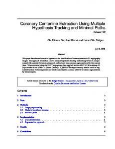
II. I NDOOR M EASUREMENTS AND C HANNEL M ODEL A. Measurement Scenario Channel measurements have been performed in an indoor scenario, a hallway at our department at Graz University of Technology [11], [12]. The transmitter mobile station (MS) was moving along a trajectory, whereas the receiver base station (BS) was fixed. The floorplan, together with the MS trajectory is illustrated in Fig. 1. The complex channel transfer function between all 381 MS positions along the trajectory and the BS has been measured with a vector network analyzer. The channel impulse responses (CIRs) for each position pk = [px,k , py,k ]T of the MS are shown in Fig. 2. Table I contains the measurement parameters. Additional information about the measurements can be found in [12].
hk(τ) / dB 6
350 −70
BS
4
300 MS
2
−80
−2
RP
time−step k
y/m
250 0 RP
−4 −6
−90 200 −100
150 100
−110
50
−120
VA
−8 −20
−15
−10
−5
0
5
10
15
x/m
0
Fig. 1. Indoor measurement scenario of the receiver base station (BS) and the trajectory of the transmitter mobile station (MS) positions (starting at p1 = [10.42, 1.45]T ). The room walls are made of concrete and plotted in black. Glass fronts are plotted in blue and metal pillars in gray. A concrete pillar is located behind the BS. The relationship between a virtual anchor (VA) and reflection point (RP) is illustrated. TABLE I M EASUREMENT S ETUP Parameter Scenario No. of MS positions Frequency range Frequency spacing Network Analyzer Antennas Antenna height
The UWB-CIR at time-step k is described by the channel model Lk X
αk,l δ(τ − τk,l ) + νk (τ ) + nk (τ ).
20
40
60
80
100 τ / ns
120
140
160
180
200
−130
Fig. 2. Measured channel impulse responses (CIRs) along the trajectory of mobile station (MS) positions. Beside the strong LOS path, many deterministic paths of strong amplitudes are visible. They originate from reflections of the transmitted signal in the environment, e.g. walls.
state-space model [13]
Value Indoor multi-storey hallway with concrete walls, large glass fronts and metal pillars 381, spacing 10 cm 6 − 8 GHz 1 MHz Rhode & Schwarz ZVA-24 Skycross SMT-3TO10M plus custom made 5-cent coin antenna 1.5 m
B. Channel and Geometric Model
hk (τ ) =
0
(1)
l=1
It is composed of a sum of Lk resolvable deterministic specular reflections with amplitudes αk,l and delays τk,l , diffuse scatters νk (τ ), as well as measurement noise nk (τ ). In (1), δ(·) is the Dirac-delta impulse. Deterministic specular reflections follow multipath geometry [2]. Floorplan information allows association of reflections to virtual sources. These so-called virtual anchors (VAs) are mirror images of the fixed anchor (here the BS). By mirroring VAs w.r.t. another reflecting surface, higher-order reflections can be taken into account naturally. Tracking the time-varying number of MPCs Lk together with their individual parameters is a challenging task as geometric visibility changes rapidly. In the following, a multi-source multi-target filter is discussed and evaluated to this problem statement.
xk = fk (xk−1 , vk ),
(2)
zk = hk (xk , nk ).
(3)
Here, zk is the observation vector, fk (·) and hk (·) are possibly non-linear functions, vk and nk are the process and observation noise. Optimal Bayesian filtering involves the propagation of the posterior probability density function (pdf) p(xk |z1:k ) forward in time. In the multi-target case, an unknown number of targets is present. Targets can appear and disappear randomly in the state-space. If a target is present, the state-space model equals the single target case described above. Multi-target filtering involves the estimation of an unknown and varying number of targets together with their states based on observations superimposed by clutter [10]. The targets present and the observations made at time k can be collected in finite-sets [6] Xk = {xk,1 , . . . , xk,Mk } ⊂ ES , (4) Zk = {zk,1 , . . . , zk,Nk } ⊂ EO .
(5)
Here, ES and EO is the state-space and observation space respectively, where the individual targets and measurements are defined. Mk is the number of targets present at time-step k and Nk is the number of observations. To model uncertainty about the number of targets and observations in each time-step k the two sets Xk and Zk are described by random finite sets. FISST allows to formulate the multi-target filtering problem within the Bayesian framework [8]. Then, optimal multi-target filtering involves the propagation of the multi-target posterior density p(Xk |Z1:k ) forward in time. A. The Probability Hypothesis Density Filter
III. M ULTI -TARGET F ILTERING A state-space description of the individual target MPCs allows to accurately model their dynamics over time. In the single-target case, the system state xk can be described by the
The PHD-Filter propagates the first-order-moment of the multi-target posterior density forward in time. This is computationally less intensive than propagating the full posterior. The number of targets present, together with their states
can be estimated from the PHD [6]. The PHD-Filter used herein, is adapted from [10] and restated here for the sake of completeness. The prediction and update equations are Dk|k−1 (xk |Z1:k−1 ) = γk (xk ) + Z φk|k−1 (xk , xk−1 )Dk−1|k−1 (xk−1 |Z1:k−1 )dxk−1 (6) and Dk|k (xk |Z1:k ) = # X ψk,z (xk ) Dk|k−1 (xk |Z1:k−1 ). ν(xk ) + κk (z) + hDk|k−1 , ψk,z i
"
z∈Zk
(7) Where, φk|k−1 (xk , xk−1 ) ν(xk ) ψk,z (xk ) κk (z)
PS (xk−1 )fk|k−1 (xk |xk−1 ) + bk|k−1 (xk |xk−1 ), = 1 − PD (xk ), = PD (xk )g(z|xk ), = λk uk (z). =
The prediction equation (6) is composed of: the PHD for spontaneous birth of a target γk (·), the probability PS (·) that a target survives from the previous time-step k −1 to the current time-step k, the single-target motion distribution fk|k−1 (·|·) described by the state-space model given in (2) and the PHD of a spawned target bk|k−1 (·|·). Note, a spawned target is a new target which appears in the state-space close to an existing target. In the update equation (7), PD (·) denotes the probability of detection, g(·|·) is the single target measurement likelihood function, λk is the Poisson parameter specifying the expected number of clutter measurements, uk (·) is the probability density over the state-space of clutter points and h·, ·i marks the inner product. Unless no special assumptions on the target dynamics are made, propagating the PHD is still computationally intractable [8]. To reduce this complexity burden, the PHD is approximated with a sequential Monte-Carlo approach. Here, the posterior pdf is represented by a set of randomly drawn samples with associated weights [13]. These particles are then propagated forward in time. B. Target State Estimation and Track Association The PHD-Filter avoids to make any data association of the individual targets. If they are of interest, then they need to be estimated from the PHD. In the case of the particle PHD-Filter, the number of targets present can be estimated by the summation of the particles weight. The individual target states are then the cluster centers obtained by clustering the particles into that number of clusters. As suggested by [10], clustering of the particles can be done by using, e.g. the kmeans algorithm. Note, an incorrectly estimated cardinality can lead to erroneous target states. To conserve target track identity along multiple time-steps, a method for target track
association of the individual targets is needed. A single target follows the single-target state-space model given in (2) and (3). This model can be used to propagate a target to the next time-step. The likelihood between the propagated target and all estimated targets within that time-step is evaluated using a likelihood function, e.g. a Gaussian normal distribution. The estimated target and the propagated target from the previous time-step are marked with the same label if the likelihood between them exceeds a given threshold. We adapted the method for target track labelling from [10]. IV. P ERFORMANCE E VALUATION A. Pre-Processing of the Measurement Data We are interested in tracking the delay of the MPCs along the MS trajectory. For that purpose, the exact time delay values τk,l of the Nk highest amplitude peaks are extracted in a search-and-subtract manner from all measured UWBCIRs using the method described in [11]. Due to the dense indoor scattering scenario, we assume Nk ≥ Lk and expect the PHD-Filter to suppress measurements caused by diffuse scatterers and measurement noise. Furthermore, we drop the time dependency of Nk = N and set it to N = 20. The set of observations Zk given in (5) for each time-step k is plotted in Fig. 3. B. Single Target State-Space Model In order to locate the VAs relative to the current MS position in the 2D-domain, we incorporate knowledge of the movement of the MS itself. In particular, the velocity vector of the MS is used. In a real application scenario this information can be obtained with, e.g. an inertial measurement unit at the MS. The position of a VA w.r.t. the MS position at time instance k is described by the system state vector xk = [rk , ϕk ]T . It is composed of the distance rk and the angle ϕk . Note, these elements are relative to the current MS position which itself is a-priori unknown. Then, the state-space model given in (2) is # " q p˜2x,k + p˜2y,k + vk , (8) fk (xk−1 , vk ) = arg (˜ px,k + j p˜y,k ) where p˜x,k = rk−1 · cos(ϕk−1 ) − ∆t · vx,k ,
(9)
p˜y,k = rk−1 · sin(ϕk−1 ) − ∆t · vy,k .
(10)
Here, we assume the process noise to follow a Gaussian normal distribution vk ∼ N (0, Σv ) with zero mean and covariance matrix Σv . The velocity of the MS in x− and y−direction is used as input into (8) denoted by vx,k and vy,k . The time-interval is denoted by ∆t. The observation equation given in (3) is then 1 rk . (11) c Here, rk is contained in the system state vector xk and c is the propagation velocity. hk (xk , nk ) =
180
300
160
250
140 time−step k
time−step k
350
200 150
120 100 Estimated Target
100 80
Estimated Target 50
Geometric Groundtruth 60
Direction Change of MS 0
Measurement
Measurement
0
20
40
60
80
100 τ / ns
120
140
160
180
Fig. 3. Time delay τ of the amplitude peaks extracted from the measurements (red dots). The delay τ of the amplitude peaks are extracted in a search-andsubtract manner from the UWB-CIRs and are used as input to the PHD-Filter. The output of the PHD-Filter the estimated targets are plotted in blue.
Direction Change of MS 5
200
10
15
20
25
30
35
40
45
50
τ / ns
Fig. 4.
Close-up view of Fig. 3 including the geometric groundtruth.
14
Geometric Groundtruth Estimated
12
Direction Change of MS 10
In order to evaluate how well the PHD-Filter performs in our measurement scenario, a groundtruth is needed. With the help of floorplan information, a geometric groundtruth of the MPCs was computed for all MS positions. This method is described in [11]. This groundtruth considers specular reflections up to the second order in the horizontal plane. Therefore, the PHDFilter may estimate more targets than actually contained in the geometric groundtruth. Part of the groundtruth is plotted in Fig. 4, its cardinality is plotted in Fig. 5. D. PHD-Filter Parameters In the PHD-Filter, the probability of survival was set to PS = 0.9. The probability of detection PD = 1, i.e. we assumed to measure all delays of the MPCs present. The clutter distribution was assumed to be uniform over the statespace with a clutter rate of λk = 17 . The single-target measurement likelihood function follows a Gaussian distribution g(·|·) ∼ N (0; 0.15 · 10−9 ). 500 particles are used to represent a target. Additionally, 100 particles are introduced into the system to model newborn targets. The newborn particles follow a uniform distribution with radius r ∼ U[0; 60] and angle ϕ ∼ U[−π; π]. The process noise of the single-target state-space model is Gaussian� with zero-mean and covariance π matrix Σv = diag 0.05, 180 . E. Estimated States and Cardinality The time delay τ of the extracted amplitude peaks from the UWB-CIRs are plotted in Fig. 3. They act as input to the PHDFilter. Additionally, the plot contains the output of the PHDFilter, which is the estimated targets. Fig. 4 provides a close-up view of Fig. 3 together with the geometric groundtruth. One can see that the estimated targets fit the geometric groundtruth very well. However, not all of the groundtruth has been estimated as target states. This can have several reasons: (i) there is no measurement in the measurement set Zk associated with same groundtruth value; (ii) the measurements fluctuate too much in τ −domain for succeeding time-steps. As a result,
Cardinality
C. Geometric Groundtruth
8 6 4 2 0
0
50
100
150
200 time−step k
250
300
350
400
Fig. 5. Cardinality estimated by the PHD-Filter compared with the cardinality of the geometric groundtruth.
the target-measurement likelihood g(·|·) is too low and no target state is estimated; (iii) there are too few measurements in succeeding time-steps to produce a valid target estimate. Estimated targets having no associated groundtruth can be seen in Fig. 4. Targets which are not part of the geometric groundtruth are e.g. third-order reflections or reflections from the floor and ceiling. An extension of the used groundtruth to higher-order reflections should validate this. Most of the targets belonging to an MPC have been estimated and most of the measurements that originated from diffuse scattering components or measurement noise are suppressed by the PHDFilter. The used state-space model is able to handle the target dynamic present in our measurement scenario. In the NLOS case between MS position k = 280 and k = 320, the PHD-Filter is also able to estimate MPCs. There are some remaining targets which only occur for one or only a few timesteps. These targets can be explained from diffuse scattering components which are not filtered out by the PHD-Filter. The number of estimated targets is plot in Fig. 5. In most cases, this number is higher than the groundtruth. A reason for this is the clutter parameter λk , which models the number of average clutter returns in the measurement set Zk . This value has been set to be constant over all MS positions, which is highly unlikely and depends strongly on the environment. Since we do not know this number in advance, it has to be set to a proper
maintained the target track for 5.8m along the MS trajectory. Another target track lives for 2.8m from MS position k = 79 until k = 107. This target track can be associated to a firstor second-order reflection.
180 160
time−step k
140
V. C ONCLUSION
120 100 Estimated Target 80
Target Track Geometric Groundtruth
60
Direction Change of MS 5
10
15
20
25
30
35
40
45
50
τ / ns
Fig. 6. Close-up view of the labelled estimated targets. The targets estimated by the PHD-Filter are associated to target tracks. Targets belonging to the same track are connected by a solid line.
value to meet the design requirements. On the one hand, a high λk enables to suppress targets with a short life-time, but might also filter out valid targets at time-steps where many VAs are present. On the other hand, if λk is set too low there might be too many targets estimated. The PHD-Filter jointly estimates the number of targets present and their individual states, but the states itself still need to be extracted from the PHD. The used k-means clustering is a simple, but not optimal approach. In the PHD-Filter, the estimated number of targets is modeled by a Poisson distribution. Therefore, the estimated number of targets from the PHD-Filter varies from one time-step to the other. For a larger number of targets present its variance is also higher. The variation in cardinality for succeeding time-steps can be well observed in Fig. 5. The target extraction step of the PHD-Filter uses the estimated cardinality to set the number of cluster centers for the k-means cluster algorithm. An erroneous number can lead to erroneous target estimates. Moreover, the k-means algorithm produces only local optima and strongly depends on the initial cluster centers. F. Traget Track Association and Labelling We are interested in identifying MPCs in the CIRs measured along the MS trajectory, which can then be associated to single VAs. For that purpose, the estimated targets are assigned to the same target track if the likelihood between them is high enough (see Sec. III-B). The used method only propagates single targets to the next time-step and computes the likelihood between the propagated and the estimated targets in that timestep. Therefore, it cannot maintain the target track if there is a single target missing along the MS trajectory. As a result, a new label will be assigned to the new target track after a missed target. Fig. 6 provides a close-up view of the labelled targets. Single targets which originated from diffuse scatterers are not assigned with a target label. Therefore, this method can be seen as an additional filtering step in estimating the MPCs along the MS trajectory. A single target track is associated between time-step k = 69 to k = 127. This corresponds to the LOS component (compare with Fig. 2). The PHD-Filter has
A method to extract and track several MPCs simultaneously along a measurement trajectory has been presented. We have shown the applicability of a multi-source multi-target filter, the so called PHD-Filter, for jointly estimating the number of MPCs together with their delays in a challenging dense indoor scattering scenario. This method is capable of keeping track of a varying number of MPCs, which is hard to achieve with perMPC tracking schemes. Most of the diffuse scattering components and measurement noise have been filtered by the PHDFilter, while most of the estimated MPCs can be matched with a geometrically obtained groundtruth considering only single and double specular reflections. Further work needs to focus on quantitative performance measures. For this purpose, higherorder reflections need to be incorporated into the groundtruth. Focus will also be put on model refinements, techniques for MPC extraction from the PHD-Filter as well as target track continuity. R EFERENCES [1] A. Molisch, Wireless Communications. John Wiley & Sons, 2005. [2] Y. Shen and M. Win, “On the Use of Multipath Geometry for Wideband Cooperative Localization,” in Global Telecommunications Conference. GLOBECOM 2009. IEEE, 2009, pp. 1–6. [3] K. Witrisal and P. Meissner, “Performance Bounds for Multipath-aided Indoor Navigation and Tracking (MINT),” in Communications, 2012. ICC ’12. IEEE International Conference on, Ottawa, Canada, 2012, accepted. [4] P. Meissner and K. Witrisal, “Multipath-assisted single-anchor indoor localization in an office environment,” in Systems, Signals and Image Processing (IWSSIP), 2012 19th International Conference on, april 2012, pp. 22–25. [5] X. Yin, G. Steinbock, G. Kirkelund, T. Pedersen, P. Blattnig, A. Jaquier, and B. Fleury, “Tracking of Time-Variant Radio Propagation Paths Using Particle Filtering,” in Communications, 2008. ICC ’08. IEEE International Conference on, may 2008, pp. 920–924. [6] K. Panta, B.-N. Vo, S. Singh, and A. Doucet, “Probability hypothesis density filter versus multiple hypothesis tracking,” Signal Processing, Sensor Fusion, and Target Recognition XIII,, vol. 5429, no. 1, pp. 284– 295, 2004. [7] S. S¨arkk¨a, A. Vehtari, and J. Lampinen, “Rao-blackwellized particle filter for multiple target tracking,” Information Fusion, vol. 8, no. 1, pp. 2–15, 2007, 7th International Conference on Information Fusion. [8] R. Mahler, Statistical multisource-multitarget information fusion. Artech House, 2007. [9] H. Sidenbladh, “Multi-target particle filtering for the probability hypothesis density,” in Information Fusion, 2003. Proceedings of the Sixth International Conference of, vol. 2, 2003, pp. 800–806. [10] D. Clark and J. Bell, “Multi-target state estimation and track continuity for the particle PHD filter,” Aerospace and Electronic Systems, IEEE Transactions on, vol. 43, no. 4, pp. 1441–1453, 2007. [11] P. Meissner, D. Arnitz, T. Gigl, and K. Witrisal, “Analysis of an indoor UWB channel for multipath-aided localization,” in Ultra-Wideband (ICUWB), 2011 IEEE International Conference on, 2011, pp. 565–569. [12] M. Froehle, P. Meissner, T. Gigl, and K. Witrisal, “Scatterer and virtual source detection for indoor UWB channels,” in Ultra-Wideband (ICUWB), 2011 IEEE International Conference on, 2011, pp. 16–20. [13] M. Arulampalam, S. Maskell, N. Gordon, and T. Clapp, “A tutorial on particle filters for online nonlinear/non-Gaussian Bayesian tracking,” Signal Processing, IEEE Transactions on, vol. 50, no. 2, pp. 174–188, 2002.