Alison L. Marsden â, Meng Wang â , J. E. Dennis, Jr. â¡ and Parviz Moin § ... on a modification of the surrogate management framework (Booker et al., 1999).
Trailing-edge noise reduction using derivative-free optimization and large-eddy simulation Alison L. Marsden ∗, Meng Wang †, J. E. Dennis, Jr. ‡ and Parviz Moin
§
revised July 10, 2006
Abstract Derivative-free optimization techniques are applied in conjunction with large-eddy simulation (LES) to reduce noise generated by turbulent flow over a hydrofoil trailingedge. A cost function proportional to the radiated acoustic power is derived based the Ffowcs Williams and Hall solution to Lighthill’s equation. Optimization is performed using the surrogate management framework with filter-based constraints for lift and drag. To make the optimization more efficient, a novel method has been developed to incorporate Reynolds-averaged Navier-Stokes (RANS) calculations for constraint evaluation. Separation of constraint and cost function computations using this method results in fewer expensive LES computations. This work demonstrates the ability to fully couple optimization to large-eddy simulation for time-accurate turbulent flow. Results demonstrate an 89% reduction in noise power, which comes about primarily by eliminating low frequency vortex shedding. The higher frequency broadband noise is reduced as well due to a subtle change of the lower surface near the trailing edge.
1
Introduction
Minimization of noise generated by the turbulent flow over a lifting surface requires advanced simulation techniques, such as large-eddy simulation, together with non-traditional optimization methods. In this work, we develop a framework for optimizing the trailing-edge of an airfoil based on a modification of the surrogate management framework (Booker et al., 1999). The present work is an extension of previous work of Marsden et al. (2004a,b), in which shape optimization was applied to minimize vortex-shedding noise from an airfoil in laminar flow. In order to meet the challenges of the turbulent flow problem, several issues are addressed. These include the derivation of an appropriate cost function for trailing-edge noise in turbulent flow, and the development of an optimization procedure that separates constraint and cost function evaluations to reduce the computation cost of the optimization. In general, when turbulent boundary layer eddies are convected past the trailing edge of a large (relative to acoustic wavelength) body, their aeroacoustic source characteristics are modified by the edge, resulting in a more efficient source type (Ffowcs Williams & Hall, 1970; Crighton & Leppington, 1971). This scattering mechanism produces strong, broadband radiation to the far-field, as discussed by Howe (1978) and Ffowcs Williams & Hall (1970). ∗
Mechanical Engineering Department, Stanford University Department of Aerospace and Mechanical Engineering, University of Notre Dame ‡ Department of Computational and Applied Mathematics, Rice University § Mechanical Engineering Department, Stanford University †
1
If there is coherent vortex shedding, typically associated with blunt trailing edges and/or high angles of attack, tonal or narrowband noise is also present (Brooks & Hodgson, 1981; Blake & Gershfeld, 1988). Additionally, it is well known that the fluctuating surface pressure may result in excitation of structural vibrations, fatigue, and low frequency noise radiation (Blake, 1986) in a phenomenon known as singing. Trailing-edge noise is a challenge in many aeronautical and naval applications, including hydrofoils, rotor blades, and airframe noise. In naval applications, hydrofoils that generate lift are used both for propulsion and as control surfaces. It has been shown by Blake (1986) that relatively small changes in the geometry of a hydrofoil trailing-edge can lead to substantial changes in the aeroacoustic performance. For example, the addition of a chamfer or knuckle to the trailing-edge can significantly modify the large scale vortex shedding in the wake, thus affecting the magnitude and spectrum of the acoustic energy generated near the trailing-edge.
1.1
Acoustic computations using large-eddy simulation
For aeroacoustics, time accurate computations such as large-eddy simulation (LES) are required to resolve the range of spatial and temporal flow scales relevant to noise generation. Several groups have performed trailing-edge computations which support the use of LES for accurate prediction of trailing-edge flow and noise. Wang & Moin (2000) have developed numerical prediction capabilities for trailing-edge noise based on LES and the Lighthill acoustic analogy, using the sharp (25◦ ) trailing edge experiment of Blake (1975) as a test case to validate the computational methods. In this approach, the acoustic field is decoupled from its hydrodynamic source field which is computed using incompressible flow equations based on the low Mach number approximation. Their simulation results have established the feasibility of the LES approach for predicting the basic statistics and structure of the velocity and surface-pressure fields in the presence of unsteady separation near the trailing-edge. The acoustic far-field was computed using Lighthill’s theory with an approximate hard-wall Green’s function following the integral formulation of Ffowcs Williams & Hall (1970). The acoustic evaluation is performed in the Fourier frequency domain. Further validation of this approach was provided by Wang (2005) who simulated a recent experiment at the University of Notre Dame (Olson & Mueller, 2004) involving a more blunt (45◦ ) trailing edge (see Figure 1). Computations have been carried out to determine the source-term characteristics and the far-field noise spectra. The variational form of the Lighthill equation has been used to compute trailing-edge noise by Oberai et al. (2002). In this work, the effect of a finite airfoil chord was studied, and the details of trailing-edge geometry could be included in the computation of far field noise.
1.2
Derivative-free optimization using surrogates
Using the computational methods of Wang & Moin (2000) and Wang (2005) as a basis, we now extend this work from noise prediction to minimization. In choosing an appropriate optimization method for the trailing-edge problem, several challenges arise. Optimization of unsteady flow problems, such as the trailing-edge noise problem, are difficult using standard gradient-based methods. Although adjoint solvers provide an efficient method of computing gradients for problems with many design variables (Jameson et al., 1998), they present data storage issues for unsteady flows and their implementation is flow-solver dependent. Additional difficulties arise with adjoint methods for constrained optimization because each constraint requires an additional adjoint equation and its solution. Derivative-free optimiza-
2
tion methods offer a viable alternative, but are often dismissed because of computational expense. In this work, we use a tailored and extended version of the surrogate management framework (SMF) developed by Booker et al. (1999) to optimize the trailing-edge shape. The SMF method is a derivative-free method which is made highly efficient by the incorporation of surrogates. Convergence of the extended SMF method comes from mesh adaptive direct search (Audet & Dennis, 2004a), and incorporates surrogate functions for increased efficiency. Several recent extensions to this method have made it more suitable for the trailing-edge problem, particularly for constrained optimization. Optimization using related methods has been performed in previous work to suppress the laminar vortex-shedding noise from an acoustically compact airfoil. A novel adaptation of the SMF method with constraints has been validated for optimal aeroacoustic shape design with constraints on lift and drag by Marsden et al. (2004a,b). These laminar flow cases validate the optimization technique for an unsteady fluid mechanics problem and demonstrate its robustness and computational efficiency.
1.3
Problem formulation and outline
We aim to minimize the broadband noise from turbulent flow over the airfoil shown in Figure 1 at a chord Reynolds number of Re = 1.9×10⁶ and a Mach number of M = 0.09. This airfoil has a beveled 45◦ trailing edge with the same geometry as on of the Blake (1975) trailing edges used previously by Marsden et al. (2004a,b) in the laminar flow cases. The leading edge is more aerodynamic, and the longer straight section allows for full development of the turbulent boundary layers. The airfoil has a chord to thickness ratio of 18, or c = 18 and h = 1 in dimensionless units (normalized by thickness). The geometry was also used in the recent Notre Dame experiments of Olson & Mueller (2004) and the companion large-eddy simulation by Wang (2005). The cost function for an acoustically non-compact airfoil is derived in Section 2. It is based on Lighthill’s theory and is proportional to the total radiated acoustic power. LES is used for source field computations. To address the high computational cost of turbulent calculations, we introduce a method to incorporate both Reynolds averaged Navier-Stokes (RANS) and LES into the optimization procedure in Section 4.1. This allows for determination of the constraint violation in advance using RANS, avoiding unnecessary costly LES evaluations when lift and drag constraints are violated. The paper is structured as follows. In Section 2 we outline the procedure used for acoustic computations, and we derive a cost function to measure the far-field noise. A general overview of the surrogate management framework for constrained optimization is presented in Section 3. The method is then extended for use in this problem in Section 4. Application of a new polling method, developed by Audet & Dennis (2004a), is presented in Section 5. Finally, results from optimization of the trailing-edge are presented and analyzed in Section 6, showing as much as 89% reduction in far-field noise. The paper concludes with discussion in Section 7.
3
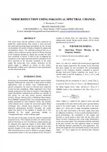
Figure 1: Airfoil shape with five trailing-edge control points used for deformation of upper and lower airfoil surface.
2 2.1
Acoustic cost function Cost function formulation
The methodology for the acoustic computations is based on the Lighthill analogy. It is desirable to use a cost function with a simple analytical form to reduce the complexity of the optimization problem. We have chosen to base the cost function on the integral solution to the Lighthill equation derived by Ffowcs Williams & Hall (1970). This solution relies on the use of a hard wall Green’s function for a semi-infinite half plane, on which the normal derivative vanishes. Formally, the use of this approximate Green’s function is justified when the foil is long and thin relative to the acoustic wavelength, i.e., when h∗ < λa < C ∗ (∗ denotes dimensional variable)or in dimensionless form, 2π 2π 0. An infeasible point x0 is considered filtered, or dominated, if there is an infeasible point x belonging to the filter for which H(x) ≤ H(x0 ) and J(x) ≤ J(x0 ). A filter, F, is defined here to be the finite set of non-dominated infeasible points plus the best feasible point found so far. Use of a filter for constrained optimization allows for identification of a set of solutions which make up the set of best points found during the optimization, rather than a single optimal shape. The filter can be viewed as sort of Pareto front showing the trade-off between obtaining a low cost function value (J axis), and satisfying constraints (H axis). The filter divides the space of J vs. H into two areas, called the unfiltered and filtered regions. Further details on the use of filters may be found in Marsden et al. (2004a). The filter is used together with the SMF method for optimization. The SMF method is a mesh based pattern search algorithm, so that all points evaluated are restricted to lie on a mesh in the parameter space. The first step is to evaluate a set of initial data for construction of the surrogates, which are Kriging functions in the present work. Initial data is chosen using Latin hypercube sampling McKay et al. (1979). Following evaluation of the initial data, the SMF algorithm consists of two steps, SEARCH and POLL. The SEARCH step provides means for local and global exploration of the parameter space, but is not strictly required for convergence. In the SEARCH step, optimization is performed on the surrogate in order to predict the location of one or more minimizing points, and the function is evaluated at these points. If a new non-dominated point is found (i.e. the filter is improved), the search is considered successful, the surrogate is updated, and another search step is performed. 8
If the SEARCH fails to find an improved point, then it is considered unsuccessful and a POLL step is performed. Convergence of the SMF algorithm is guaranteed by the POLL step, in which points neighboring the current best point on the mesh are evaluated in a positive spanning set of directions to check whether the current best point is a mesh local optimizer. If the POLL produces an improvement in either the best feasible or least infeasible point, then the next SEARCH step is performed on the current mesh. Otherwise, the current best point is a local minimizer of the function on the mesh. For greater accuracy, the mesh may be refined, at which point the algorithm continues with a SEARCH. Convergence is reached when a local minimum on the mesh is found, and the mesh has been refined to the desired accuracy. Each time new data points are found in a SEARCH or POLL step, the data is added to the surrogate and it is updated.
4 4.1
Optimization procedure Incorporation of RANS and LES in optimization
In extending the trailing-edge optimization from laminar to turbulent flow, the main challenge is one of increased computational cost. The cost of the LES is such that it is not practically feasible to simulate the entire airfoil, and instead computations are performed in a truncated domain that includes only the trailing-edge portion of the airfoil. This makes it impossible to integrate lift and drag values over the entire airfoil surface in the LES computation. LES is used to compute the cost function by integrating the acoustic source in the trailing-edge region. The large computational cost of doing optimization using LES-based function evaluations can be mitigated by incorporating RANS into the optimization procedure. While it is not possible to obtain accurate acoustic predictions from RANS, reasonably accurate aerodynamic data, including mean lift and drag values, can be readily obtained. A steady RANS simulation of the entire airfoil requires only 5 single processor SGI O3K CPU hours using the commercial package Fluent. Incompressible RANS computations are performed on a C-type mesh using the Spalart-Almaras turbulence model. Because of the orders of magnitude disparity in simulation time between RANS and LES, it is advantageous to use RANS calculations whenever possible and to reduce the number and size of full LES simulations. In addition to computing lift and drag, the RANS method is used to provide boundary conditions for the LES simulation. The domains for the RANS and LES simulations are shown in Figure 3. The larger domain, including the full airfoil, is used for the steady RANS simulations. Mean velocity boundary conditions are then interpolated from the RANS results onto the smaller rectangular LES domain. LES is performed in a separate computation using the boundary conditions provided by the RANS. The smaller LES domain includes only the trailing-edge portion of the airfoil. In addition, the LES code is equipped with a turbulent inflow generation capability employing the “rescale and recycle” technique of Lund et al. (1998). With this method the inflow turbulent boundary data are generated on the fly as the simulation proceeds (see Wang (2005)). Using the RANS simulation to compute lift and drag, it is possible to check the constraint violation function value H before starting a full LES simulation of a given airfoil shape, and to avoid doing the LES if the violation is too large. Decoupling the constraint computation from the cost function computation offers a large savings in computational cost because unneeded expensive LES simulations can be avoided. In LES, a hybrid finite-difference/spectral code described in Wang & Moin (2000) is used 9
Figure 3: Domains used for RANS computations (thick line) and LES computations (thin line).
10
to solve the spatially filtered, time-dependent, incompressible Navier-Stokes equations in generalized curvilinear coordinates. The subgrid-scale (SGS) stress tensor is modeled by the dynamic Smagorinsky model (Germano et al., 1991; Lilly, 1992). The mesh size used in the LES computation is 1540×96×48, for a total of about 7 million mesh points. Each evaluation of the cost function using LES takes approximately 2000 single-processor hours on an IBM SP4. This allows for the removal of initial transients and sufficiently long sampling period for statistical convergence of the acoustic spectrum and the cost function value. Convergence of the cost function is discussed in Section 6.1. The procedure that has been implemented to incorporate LES and RANS into the optimization algorithm is outlined below. In practice, the optimization routine outputs a set of parameter values representing a unique airfoil shape. These parameter values are taken as inputs in a series of automated scripts which then generate the airfoil geometry, computational mesh, and run the RANS and LES calculations. The steps that are outlined below constitute one function evaluation in the optimization algorithm. A RANS simulation is required to evaluate the constraint violation as part of every function evaluation. Depending on the constraint violation function value, an LES computation may or may not be performed to determine the cost function value for a given airfoil shape. The steps in computing the cost function and constraint violation function are summarized as follows: 1. The shape parameters are used to define the airfoil geometry and corresponding trailingedge surface mesh. A C-mesh is generated for the RANS computation (using every other trailing-edge surface point), and a truncated domain mesh is generated for the LES computation. 2. A steady RANS computation is performed using the Spalart-Allmaras turbulence model to obtain coefficients of lift and drag. 3. The constraint violation function H (Eq. (13)) is computed using RANS lift and drag data to determine if H ≤ Hmax , the maximum allowable value. 4. If H ≤ Hmax , the constraint violation is within the acceptable limit, and the point may be included in the filter. Proceed to steps 5, 6, and 7. Else, if H > Hmax , LES is not performed. The point is rejected and the value of J for this shape is set to infinity. 5. Mean velocity boundary conditions are interpolated from RANS solution onto the boundary of the LES domain (Figure 3). 6. LES is performed using interpolated boundary conditions from RANS plus turbulent boundary layer generation as input. The volume integral of Equation (5) is evaluated to obtain the acoustic source. 7. The intergral of the acoustic spectrum, equal to the cost function value J, is computed in a post processing step following the procedure in Section 2. Since the cost function and the constraint violation function are computed separately, it is possible to use a filter with a very small value of Hmax , and avoid doing an expensive LES simulation if H falls outside the region included in the filter. In the laminar trailing-edge problem, the filter proved to be extremely valuable in identifying a range of possible solutions, and it was shown that a large reduction in cost function could be achieved with only a small 11
constraint violation. Based on results of the laminar case, we choose a value of Hmax that is small enough to exclude large constraint violations, but large enough to identify shapes that may offer significant further cost function reduction. Using the above method, there are many fewer points where the cost function value J is known (from LES) than points where H is known (from RANS). We therefore construct one surrogate to approximate J, and another to approximate H. In this way, the surrogate for the constraint function values (H) can incorporate all solutions found by the RANS, even if H > Hmax and no corresponding J value was computed for that point. To search the parameter space, the surrogates can be summed with a penalty as follows Jˆ = J + αH,
(14)
where α is a parameter that is systematically updated using the filter at each iteration. This is a slight change from the laminar case presented in Marsden et al. (2004a), in which a single ˆ surrogate was constructed to approximate J. The large cost of turbulent flow simulations makes parallelization of the optimization even more crucial than in the laminar flow case. During any SEARCH or POLL step, several points are evaluated in parallel using RANS and LES. Given the large cost of a single LES solution, if it was not possible to simultaneously evaluate several trailing-edge shapes, this problem would quickly become intractable. In the above formulation, we allow for the rejection of points that do not satisfy the constraint violation requirement. Formally, rejection of infeasible points is allowed within the convergence theory because of a new polling method which has been implemented for the turbulent case. Mesh adaptive direct search (MADS) was developed by Audet & Dennis (2004a), and it offers several advantages over the pattern search polling that was used in the laminar case. This new polling method is discussed in the following section.
5
Mesh adaptive direct search
Mesh adaptive direct search (Audet & Dennis, 2004a) is a new method for choosing poll directions that offers greater flexibility than generalized pattern search (GPS) polling, and is capable of generating a dense set of directions. To have a dense set of polling directions means that as the mesh becomes infinitely fine, the number of possible poll directions approaches infinity. The possibility of generating a dense set of poll directions makes for a much stronger convergence theory, especially with regard to nonlinear constraints. We refer the reader to Audet & Dennis (2004a) for more details and proof of convergence. The main idea behind MADS is the introduction of a frame size parameter that evolves separately from the mesh size. In addition to the mesh size parameter ∆m k , the poll size parameter ∆pk is introduced. The poll size parameter is used to define a frame around the poll center which contains all points which may be used to define a poll direction. Figures 4 and 5 illustrate the difference between GPS and MADS polling. Figure 4 shows a sequence of successively finer meshes, and corresponding GPS poll sets in two dimensions. In the case of GPS polling, the number of points contained in the frame (bold line outlined box) remains constant (9 in this example) as the mesh is refined. In contrast, Figure 5 shows a sequence of three successively finer meshes used for MADS polling. As the mesh is refined, each time by 1/4, the frame size shrinks more slowly, so that with each refinement the frame contains more points which can be used to define a poll direction. With this illustration, we see that the number of possible poll directions increases as the mesh is refined. 12
p ∆m k = ∆k = 1 p1
p ∆m k = ∆k =
1 2
p ∆m k = ∆k =
1 4
s sp2 p1 s
s p2
sx
k
sp3
s @
p2 s
xk
@ @ @sp1
xk
s @ @3 s p
s p3
1 2 3 Figure 4: Example of GPS frames Pk = {xk + ∆m k d : d ∈ Dk } = {p , p , p } for different p m values of ∆k = ∆k . In all three figures, the mesh Mk is the intersection of all lines.
Even without refining the mesh, MADS offers an advantage over GPS when ∆m k < 1 by allowing for a larger number of directions to be represented. By performing a series of POLL steps, a more complete local search of the parameter space around the poll center results. Additionally, the fact that MADS can generate a dense set of poll directions means that it that it will automatically conform to the boundary of the parameter space when polling on or near the boundary. Polling near the boundary of the domain therefore requires only n + 1 poll points. The MADS method also offers advantages in convergence for constrained optimization. In a non-linearly constrained optimization problem, the boundary shape of the feasible region is unknown. Because GPS polling is limited to a finite set of directions, it is not guaranteed that the polling directions will conform to boundary, and may miss the descent direction unless conforming directions are added. In contrast, MADS polling guarantees that a poll point will eventually land in the descent direction because the poll directions will fill the space as the number of mesh refinements approaches infinity. This difference makes it possible to use the barrier approach to constraints together with MADS polling, in which the cost function value is simply set to infinity if constraints are violated. There is a trade-off between using a filter and barrier approach for constraints in the trailing-edge problem. On the one hand, using a barrier approach would result in fewer expensive LES simulations because LES would never be performed when lift and drag constraints were violated. On the other hand, a filter allows for identification of solutions with a very small constraint violation which may result in large cost function reductions. An attractive middle ground is to use a filter with a small value of Hmax , as done in the present work.
6
Results
In this section we present results for turbulent flow shape optimization using the methods described in the preceding sections. We begin by discussing convergence of the cost function in turbulent flow. We then evaluate two optimal shapes found in the laminar flow case
13
p ∆m k = 1, ∆k = 1 p3
s p1
sx
p 1 ∆m k = 4 , ∆k = 1
∆m k =
p 1 16 , ∆k
=
1 2
s s3
p
sx �
k � � s�1
k
p
sp2
ps1
S Ss s2 � xk p s� 3 p
s p2
Figure 5: Examples of MADS polling. (in Marsden et al. (2004b)) to determine if they also reduce noise in turbulent flow. It is determined that only one of the two shapes results in noise reduction in turbulent flow. These shapes are used as a starting point for the turbulent flow optimization. Finally, results using the extended SMF method in fully turbulent flow are shown to result in significant noise reduction. In the turbulent flow case, we optimize both sides of the trailing-edge using five shape parameters. The geometry and control points for optimization are shown in Figure 1.
6.1
Cost function convergence
Since the cost function value is used as the baseline of comparison for the optimization, we study the convergence and sensitivity of the cost function value for the original shape before proceeding with the optimization. The spectrum j(ω) for the original airfoil was calculated using three different values of sampling window size, n = 256, 512, 1024. The cost function J, as defined in Section 2, is the integral of j(ω). It was found that a sample size of n = 256 was not sufficient to capture the peak shedding frequency which is captured by the two larger sample sizes. However, the cost function values using these three window sizes differed from each other by no more than 5%. The larger window size of n = 1024 did the best job of capturing the peak shedding frequency, but requires significantly more samples to converge the low frequency range of the spectrum. A window size of 512 was chosen since it is sufficient to capture all frequencies of interest, and the low frequency range converges with a reasonable number of samples. Using this window size, the peak shedding frequency is approximately ω = 2.2. Figure 6 shows the time history of the three terms in the acoustic source, Srr (upper), Sθθ (middle) and Srθ (lower), from (5), starting the simulation from t = 0. We see an initial period of transience, before the flow reaches statistically steady state at around t = 50. Starting at this point, samples are collected for the cost function computation until the cost function value converges after two to three flow through times. One flow-through time across the computational domain consists of approximately 20 non-dimensional time units.
14
0.75 0.5 0.25 0
S(t)
-0.25 -0.5 -0.75 -1 25
50
75
100
t
Figure 6: Time history of three components of acoustic source Srr (upper), Sθθ (middle) and Srθ (lower), with computation starting from time t = 0. Collection of samples for cost function computation starts at t ≈ 50 after the initial transients have been washed out. One flow through time is approximately 20 non-dimensional time units.
15
Best feasible point Least infeasible point
laminar turbulent laminar turbulent
flow flow flow flow
noise -48% -39% -70% +18%
lift +229% +25% +262% +78%
drag -4% -16% +1.5% +6.6%
Table 1: Comparison of cost function, lift and drag results for two shapes in laminar and turbulent flow. Shapes were previously found to be optimal for laminar flow noise reduction with lift and drag constraints.
6.2
Comparison of laminar and turbulent solutions
In previous work of Marsden et al. (2004b), optimal shapes were identified for suppression of vortex shedding noise in laminar flow. In particular, two optimal shapes, the best feasible and least infeasible, were identified when deforming both sides of the trailing edge with constraints. In this section, we study the noise generated by these two shapes in turbulent flow to determine what, if any, correlation is found between shapes that reduce noise in laminar and turbulent flows. These results also serve as a starting point for optimization in turbulent flow. A comparison of relative changes in noise, lift and drag for the best feasible and least infeasible shapes for the laminar and turbulent flows is presented in Table 1. The values given in the table are relative to the original shape, and they show that changes in lift and drag have the same sign (although different magnitudes) for both shapes under consideration. Noise levels have decreased in both laminar and turbulent flow for the best feasible shape, and constraints are satisfied in both cases. As shown in the table, the best feasible shape resulted in a cost function decrease of 48% in laminar flow, and a decrease of 39% in turbulent flow. In contrast, the least infeasible shape from the laminar flow case caused an 18% increase of noise level in turbulent flow, where the same shape had resulted in a 70% decrease in laminar flow. Constraints for this shape in turbulent flow are not satisfied, as drag has increase by about 7%. Streamwise velocity contours in turbulent flow for the original shape and the laminar best feasible and least infeasible shapes are shown in Figure 7. The original shape (shown at the top) produces large scale vortex shedding together with smaller scale fluctuations. We observe that the shedding has been suppressed in the middle plot, corresponding to the laminar best feasible shape. As a result, the wake is thinner. The suppression of vortex shedding is consistent with the reduction of noise. The lower plot in the figure shows velocity contours for the laminar least infeasible shape. We observe that the thickness of the wake is decreased, but there are still significant large vortical structures in the near wake region. In laminar flow, the noise suppression for this shape was due to a rearrangement of vortex shedding which causes a cancellation of unsteady forces induced by the shedding vortex pairs. In turbulent flow, this mechanism does not appear to be present and the presence of smaller scale flow structures contributes significantly to the overall noise. The corresponding acoustic power spectra j(ω) are shown in Figure 8, with the original shape shown by the solid line, the laminar best feasible shape shown by the dashed line, and the least infeasible shape shown by the dash dot line. The acoustic cost function measures the integral of the curves shown over all frequencies. Compared to the original, the area under the curve has decreased for the best feasible shape but has increased for the least infeasible 16
Figure 7: Comparison of instantaneous streamwise velocity contours for original (top), laminar best feasible (center) and least infeasible (lower) shapes in turbulent flow. The best feasible shape eliminates vortex shedding compared to the original. Maximum velocity 1.36, minimum -0.60, 15 contour levels. shape. We observe in Figure 8 a decrease in spectral level at low frequencies because of the elimination of vortex shedding for the best feasible shape. For the same case, we also observe a decrease in higher frequency noise. There is a slight increase in spectral level in the midrange of frequencies compared to the original. These results correspond to the reduction in cost function of 39% for this case. In the spectrum for the least infeasible shape, we observe a significant decrease in the vortex-shedding peak. However, we also observe an increase in spectral level in the mid range and higher frequencies. In particular there is a significantly stronger secondary peak caused by a more intense shear layer emanating from the lower surface boundary layer (see Fig. 7). The overall result is an increase in total acoustic power of 18% for this case compared to the original shape. Based on these results, we conclude that (not surprisingly) a shape which reduces noise in laminar flow will not necessarily reduce noise in turbulent flow, and may even increase it. An optimization in laminar flow cannot be used to predict noise reduction in turbulent flow. However, there does seem to be a correlation in reduction of large scale vortex shedding in laminar and turbulent flow. It seems likely that a shape which reduces large scale shedding in laminar flow will also do so in turbulent flow. These results suggest that a laminar flow optimization may be a useful starting point for turbulent flow optimization if removing the
17
10
-7
10
-8
10
-9
j(ω) 10
-10
10-11 10-12 10
-13
10
1
10
2
ω
Figure 8: Comparison of noise spectra for original (—), laminar least infeasible (-·-) and laminar best feasible (- - -) shapes in turbulent flow. The cost function (integral over all frequencies) has decreased for the best feasible case compared to the original but has increased for the least infeasible case.
18
vortex shedding noise is the main objective, especially when accounting for difference in computational cost between laminar and turbulent flow simulations.
6.3
Optimal shapes for turbulent flow
The tools described in the preceding sections are combined to optimize the trailing-edge shape in fully turbulent flow. We use the extended SMF method for optimization with MADS polling and filter-based constraints. This procedure is adapted for turbulent flow by incorporating both RANS and LES to separate constraint and cost function evaluations. Based on the results of the previous section, we include the laminar flow shapes in the initial data set as a starting point for turbulent flow optimization. The final result is an optimal shape that reduces trailing-edge noise power by 89% and satisfies lift and drag constraints. The initial data set for optimization with the SMF method consisted of the same 15 points that were used in the laminar flow cases, found with Latin hypercube sampling. In addition, the two optimal shapes (best feasible and least infeasible) from the laminar flow case were included in the initial data set, for a total of 17 initial shapes. Constraint violation values (H) were found for each shape in the initial data set using RANS. Although none of the initial 15 data points satisfied the constraint criterion of H ≤ Hmax , the points with the four lowest values of H plus the two laminar flow shapes were chosen to build an initial surrogate for the cost function. All points were included in the initial surrogate for the constraints. Initial data showed that none of the 4 initial shapes evaluated with the LES resulted in a reduced cost function. In contrast, in the laminar flow optimization, two of the same shapes produces a significant reduction in cost function. The only shape that produced a reduction in turbulent flow before the first iteration was the best feasible shape from laminar flow. The filter for the turbulent optimization problem is constructed with a maximum constraint violation value of Hmax = 0.04, where H is defined as in the laminar flow case by (13). The value of Hmax was chosen to avoid unnecessary cost function evaluations using LES, while still allowing for shapes which may have a slight constraint violation but a low cost function value. The initial filter, including all initial data, the original shape, and the two laminar flow solutions, is shown on the left side of Figure 9. The solid vertical line marks the cut-off for H ≤ Hmax . Initially, there are two feasible points shown on the H = 0 axis. The feasible point shown by the star corresponds to the original shape. There is one feasible point in the filter in addition to the original shape which is marked by the square, and this point corresponds to the best feasible shape from the laminar flow case. At the start of the optimization, the initial MADS mesh size parameter is chosen to be 14 since the computational cost prohibits us from doing more than one mesh refinement. Starting MADS using a mesh size parameter of 1 would be equivalent to GPS in the first iteration, and MADS would not offer any advantages over GPS polling until the mesh is refined. After only one SEARCH step of the extended SMF method, a shape which results in 85% noise reduction was identified by the surrogate. This shape exactly satisfies the constraints, with a lift increase of 64% and a drag decrease of 15% compared to the original. The number of RANS evaluations required was 21, including 15 initial points, the original shape, two laminar flow shapes and three SEARCH points. The corresponding number of LES evaluations was 8, since only 4 of the 15 initial points were evaluated using LES, and only one of the SEARCH points satisfied H ≤ Hmax . After three iterations, a shape resulting in an 89% reduction in noise was identified. 19
−5
3.5
−5
x 10
3.5
3
3
2.5
2.5
2
2
J
x 10
J 1.5
1.5
1
1
0.5
0.5
0
0
0.05
0.1
0.15
0.2
0
0.25
0
0.05
0.1
H
0.15
0.2
H
Figure 9: Initial filter (left) and filter after third iteration (right) for turbulent flow optimization. Cost function J vs. constraint violation function H. The solid vertical line shows the cut-off for H ≤ Hmax . noise -85% -89%
lift +64% +63%
drag -15% -16.5%
RANS evaluations 21 30
LES evaluations 8 16
iterations 1 3
Table 2: Optimization results for turbulent flow. The first row shows results after the first iteration. An 89% reduction in noise has been achieved after only three iterations (shown in the second row).
This shape is compared to the original in Figure 10. We observe that the trailing-edge has been moved downward slightly and that the trailing-edge angle has been significantly reduced. The shapes resulting from iterations 1 and 3 are qualitatively similar. However the shape corresponding to 89% noise reduction has a slightly smaller downward deflection in the trailing-edge, and is more streamlined on the lower surface compared to the shape found in iteration 1. Constraints for the 89% reduction shape are satisfied, with a lift increase of 63% and a drag decrease of 16.5%. The computational cost breakdown is shown in Table 2 along with a summary of the cost function and constraint values at iterations 1 and 3. The total number of LES evaluations has increased to 16 by iteration three. The total number of RANS evaluations after the third iteration was 30. These results suggest that if RANS had not been incorporated into the optimization procedure, the computational cost would have been much higher. Not only would the number of LES evaluations have to nearly double, but the LES domain size would have to include the entire airfoil to allow an evaluation of lift and drag. An additional SEARCH step (iteration four) produced no further cost reduction. A plot of cost function reduction vs. number of LES evaluations is shown on the right side of Figure 10. Contours of streamwise velocity are shown for the original (top) and best feasible turbulent shape (bottom) after three iterations in Figure 11. We observe that large scale vortex shedding has been suppressed and that the wake thickness is reduced significantly compared to the original. The noise spectrum corresponding to this shape is shown together with the
20
0.25
1 0.9 0.8 0.7 0.6
J
0.5 0.4 0.3 0.2 0.1 0 0
2
4
6
8
10
12
14
16
18
NLES Figure 10: Left: Original shape (thin line) and best feasible shape (thick line) for turbulent flow optimization. This shape results in 89% reduction in total acoustic power. The corresponding spectra are shown in Figure 12. Right: Normalized cost function vs. number of LES evaluations for four iterations until convergence. original in Figure 12. The spectral level for the modified shape (– · –) shows a drastic reduction at low frequencies due to the elimination of vortex shedding. The mid-range and higher frequency noise has also been reduced compared to original shape (—). The reduction in high frequency noise is caused by a slight upturn of the lower surface toward the trailing edge, which results in a small adverse pressure gradient in the boundary layer. This in turn leads to a less intense shear layer eminating from the lower surface and reduced small scale turbulence fluctuations. These observations are validated by further examination of the flow in the trailing-edge region. Contours of the Reynolds stress components normal to the trailing edge, huui, hvvi and huvi, are shown in Figure 13. A comparison of results for the original shape (top plots) and optimized shape (bottom plots) shows much reduced levels of velocity fluctuations and turbulent shear stress in both the upper and lower shear layers, largely due to the removal of vortex shedding. These three Reynolds stress components are directly related to the three source terms in the Ffowcs Williams-Hall equation (cf. (2)–(5)). The latter are instantaneous Reynolds stresses represented in a cylindrical coordinate system. Hence, the reduction in time-averaged Reynolds stresses demonstrated in Figure 13 corresponds to a reduction in the overall acoustic source magnitude. Plots of pressure and skin-friction coefficients Cp and Cf are shown on the left and right of Figure 14, respectively. This data confirms the presence of a small adverse pressure gradient region on the pressure (lower) side near the trailing edge for the optimized airfoil. This weakens the vorticity (lower Cf magnitude), thickens the boundary layer, and therefore generates less high frequency noise. The discontinuities in Cf and in the slope of the Cp curve at about x = −5 are caused by the discontinuous slope of the airfoil surface resulting from geometry parameterization. Likewise, the 4 slope discontinuities on the Cf curve are due to the discontinuous second derivatives of the splines at the control points. Pressure side boundary layer thickening near the trailing edge in the optimal case is also observed in the mean streamwise velocity profiles shown in Figure 15. The suction side profiles clearly show a separated flow for the original shape, which is also obvious in the Cf plot, and an attached flow in the optimized case. Profiles in the near wake region, on
21
Figure 11: Contours of instantaneous streamwise velocity for original shape (top) and best feasible shape after three iterations (bottom), giving 89% noise reduction. Maximum velocity 1.29, minimum -0.32, 15 contour levels.
j(ω)
10
-6
10
-7
10
-8
10-9 10
-10
10
-11
10
-12
10
-13
101
102
ω
Figure 12: Noise spectrum for the optimized shape (– · –) compared to original shape (—) in turbulent flow optimization. The cost function is the integral over all frequencies, and we confirm that the best feasible shape results in a significant reduction (89%) in noise power. The corresponding trailing-edge shapes are shown in Figure 11.
22
Figure 13: Contours of Reynolds stress components huui (left) (min = 0, max = 0.052, 15 levels), hvvi (center) (min = 0, max = 0.05, 20 levels), and huvi (right) (min = 0, max = 0.015, 20 levels). Comparison of top plots (original shape) and bottom plots (optimized shape) shows reduced velocity fluctuations and Reynolds shear stress in both the upper and lower shear layers, largely due to the removal of vortex shedding. the right side of the figure, show a narrowing of the wake in the optimal case compared to the original due to a lack of boundary-layer separation and vortex shedding. Weakening of the shear layers in the region of the trailing edge results in smaller velocity fluctuations and reduced far field noise in the optimized case (where vortex shedding has been suppressed) compared to the original (with vortex shedding). It should be pointed out that the main objective of this work is to demonstrate conceptually that, by combining LES with the derivative-free SMF technique, we can perform difficult aeroacoustic shape design with realistic constraints at fully-turbulent Reynolds numbers. An analysis of the flow field corresponding to the optimized shape confirms that the noise-generating features of the trailing-edge flow have been eliminated or weakened significantly. Given the exploratory nature of this work, the problem set-up is somewhat idealized. The Blake airfoil was originally designed to study trailing-edge noise and was not meant to be quiet. Therefore, the large amount of noise reduction achieved by optimization, mainly through suppression of vortex shedding, is not surprising. If we had started from a more streamlined airfoil shape with a sharper trailing edge, the reduction could be less drastic (this is not always true as shown by the case of the laminar least-infeasible shape in turbulent flow, shown in Figs. 7 and 8, which is more streamlined but noisier than the original). In a realistic application, optimization is generally performed on the entire airfoil instead of only the trailing-edge portion of the airfoil, and the angle of attack is often adjusted to maintain lift. Our approach is equally valid in this case, although such an optimization has not been performed due to computational expense.
7
Summary
Results of this work demonstrate the successful coupling of shape optimization to a timeaccurate turbulent flow calculation using LES. The use of novel derivative-free optimization techniques have provided a flexible optimization framework which can be applied to a wide variety of complex flow problems. Optimization has demonstrated as much as 89% reduction in trailing-edge noise power for the shape studied in this work. Optimization for trailing-edge noise reduction presented several challenges which are not present in the laminar flow case. First, a cost function needed to be defined since the airfoil 23
0.006
0.2
0.004 0 0.002
Cp
Cf
-0.2
0 -0.4 -0.002
-0.6
-0.004 -8
-6
x
-4
-2
-8
-6
x
-4
-2
Figure 14: Coefficient of pressure (Cp ) on left and coefficient of friction (Cf ) on right for original trailing edge shape (−) and optimized shape (− · −). is not acoustically compact for the broadband noise at all frequencies. The cost function, proportional to the radiated acoustic power, was derived based on a simplified form of the Ffowcs Williams & Hall (1970) solution to the Lighthill equation as described by Wang & Moin (2000). It involves Lighthill stress source terms instead of compact surface dipoles. Aside from the cost function definition, the main challenge in the turbulent flow optimization was one of increased computational cost. A novel method to incorporate both the LES and RANS simulations in the optimization was proposed and demonstrated. Using this method, computation of the lift and drag values was done using a RANS simulation of the entire airfoil, and the constraint violation was computed in advance of doing a full LES computation. This method results in a large savings in cost by avoiding unnecessary LES evaluations in cases when constraints are violated. The optimization method was also extended to incorporate a new polling method for the turbulent flow case. Mesh adaptive direct search (MADS) offers increased effectiveness and efficiency. The application of MADS to the trailing-edge problem represented its first (known to date) use in an expensive engineering application. Analysis of a set of initial shapes in turbulent flow illustrated that shapes which reduce noise in laminar flow do not necessarily reduce noise in turbulent flow. There appears to be little correlation between noise reducing shapes in laminar and turbulent flows. Additionally, there can be a trade-off in turbulent flow between reduction in high and low frequency noise. However, results do suggest that optimization in laminar flow may serve as a useful starting point for turbulent flow optimization. Inclusion of laminar flow solutions in the initial surrogate likely resulted in faster identification of a noise reducing shape in turbulent flow. In the first iteration of the extended SMF algorithm for turbulent flow, a shape that achieved an 85% noise reduction with zero constraint violation was identified. The optimal solution produced a shape which reduced trailing-edge noise by 89% in turbulent flow while maintaining lift and drag at desirable levels. These results validate the use of the current methods for constrained optimization which may be applied to other complex flow problems. The acoustic spectrum showed a large decrease in low frequency noise because large scale vortex shedding was suppressed, and the wake was significantly narrowed. The resulting
24
0.6
0.6
0.6
0.6
2
0.5
0.4
0.4
0.4
2
2
0.4
.5
0.3
1 0.2
0.2
1
1
0.2
.5
0.1
0
0.5 1
0
0
0.5
1
0
0
0 0.5 1
0
0 0.5 1
y/h
(y − ywall )/h
0.2
0
0
0
0
0
.5
-0.1
-0.2
-0.2
-0.2
-0.2
-1
-1
-1
-0.3
.5 -0.4
-0.4
-0.4
-0.4
-2 0
-0.5
0.5
1
-2 0
0.5
1
-2 0
0.5
1
U/U0 -0.6
0.5 1
-0.6
0.5
1
-0.6
0.5
1
-0.6
0.5
1
U/U0 Figure 15: Mean streamwise velocity profiles for original shape (−), with vortex shedding, and optimized shape (− · −), without vortex shedding. Velocity profiles from upper (suction) side and lower (pressure) side are shown on the top and bottom of the left side of the figure respectively at locations x/h = −1.5, −1, −0.5 and −0.25 from left to right. Wake profiles at locations x/h = 0, 0.5 and 1.0 are shown on the right side of the figure. The optimized case exhibits a narrower wake and weaker shear layers.
25
shape is more streamlined than the original, and has a smaller trailing-edge tip angle. In addition, a slight upturn of the lower surface toward the trailing edge causes a less intense shear layer and weakened higher frequency noise. Finally, it is interesting to contrast the main noise reduction mechanisms observed in the laminar flow optimization (Marsden et al., 2004a,b) and the present turbulent flow optimization. In the laminar case, the shape optimization was unable to suppress vortex shedding, and noise suppression was instead achieved through a modification of the vortex shedding process to obtain a concellation of unsteady forces induced by the vortices from the upper and lower shear layers. In the turbulent trailing-edge flow, on the other hand, noise suppression is obtained primarily by the elimination of vortex shedding.
Acknowledgments This work was supported by ONR under grant N00014-01-1-0423 with Ronald Joslin as program manager. Computer time was provided by the DoD’s HPCMP through NRL-DC and ARL/MSRC. John Dennis was supported by the AFOSR, DOE, the IMA, the NSF, and the Ordway Endowment at the University of Minnesota. The authors also wish to thank Charles Audet and Mark Abramson for their input and helpful discussions.
References Audet, C., Booker, A. J., Dennis, Jr., J. E., Frank, P. D. & Moore, D. W. 2000 A surrogate-model-based method for constrained optimization. AIAA Paper 2000– 4891, Presented at the 8th AIAA/ISSMO Symposium on Multidisciplinary Analysis and Optimization, Long Beach, California. Audet, C. & Dennis, Jr., J. E. 2004a Mesh adaptive direct search algorithms for con´ strained optimization. Tech. Rep. G–2004–04. Les Cahiers du GERAD, Ecole Polytechnique de Montr´eal, D´epartement de Math´ematiques et de G´enie Industriel, C.P. 6079, Centreville, Montr´eal (Qu´ebec), H3C 3A7 Canada. Audet, C. & Dennis, Jr., J. E. 2004b A pattern search filter method for nonlinear programming without derivatives. SIAM Journal on Optimization 14 (4), 980–1010. Blake, W. K. 1975 A statistical description of pressure and velocity fields at the trailing edge of a flat strut. DTNSRDC Report 4241. David Taylor Naval Ship R & D Center, Bethesda, Maryland. Blake, W. K. 1986 Mechanics of flow-induced sound and vibration, Vol. I and II . London: Academic Press. Blake, W. K. & Gershfeld, J. L. 1988 The aeroacoustics of trailing edges. In Frontiers in Experimental Fluid Mechanics (ed. M. Gad-el Hak), chap. 10. Springer-Verlag. Booker, A. J., Dennis, Jr., J. E., Frank, P. D., Serafini, D. B., Torczon, V. & Trosset, M. W. 1999 A rigorous framework for optimization of expensive functions by surrogates. Structural Optimization 17 (1), 1–13. Brooks, T. F. & Hodgson, T. H. 1981 Trailing edge noise prediction from measured surface pressures. J. Sound and Vib. 78, 69–117. 26
Crighton, D. G. & Leppington, F. G. 1971 On the scattering of aerodynamic noise. Journal of Fluid Mechanics 46, 557–597. Ffowcs Williams, J. E. & Hall, L. H. 1970 Aerodynamic sound generation by turbulent flow in the vicinity of a scattering half plane. Journal of Fluid Mechanics 40, 657–670. Fletcher, R. & Leyffer, S. 2002 Nonlinear programming without a penalty function. Mathematical Programming 91, 239–269. Germano, M., Piomelli, U., Moin, P. & Cabot, W. 1991 A dynamic subgrid-scale eddy-viscosity model. Physics of Fluids A 3, 1760–1765. Goldstein, M. E. 1976 Aeroacoustics. New York: McGraw-Hill. Howe, M. S. 1978 A review of the theory of trailing edge noise. J. Sound and Vib. 61 (3), 437–465. Howe, M. S. 2001 Edge-source acoustic Green’s function for an airfoil of arbitrary chord, with application to trailing edge noise. Quarterly Journal of Mechanics and Applied Mathematics 50 (1), 139–155. Jameson, A., Martinelli, L. & Pierce, N. A. 1998 Optimum aerodynamic design using the Navier-Stokes equations. Theoret. Comp. Fluid Dynamics 10, 213–237. Lilly, D. 1992 A proposed modification of the Germano subgrid-scale closure method. Physics of Fluids 4, 633–635. Lund, T. S., Wu, X. & Squires, K. 1998 Generation of turbulent inflow data for spatiallydeveloping boundary layer simulations. J. Comput. Phys. 140, 233–258. Marsden, A. L., Wang, M., Dennis, Jr., J. E. & Moin, P. 2004a Optimal aeroacoustic shape design using the surrogate management framework. Optimization and Engineering 5 (2), 235–262, special Issue: Surrogate Optimization. Marsden, A. L., Wang, M., Dennis, Jr., J. E. & Moin, P. 2004b Suppression of airfoil vortex-shedding noise via derivative-free optimization. Physics of Fluids 16 (10), L83–L86. McKay, M. D., Conover, W. J. & Beckman, R. J. 1979 A comparison of three methods for selecting values of input variables in the analysis of output from a computer code. Technometrics 21, 239–245. Oberai, A. A., Roknaldin, F. & Hughes, T. J. R. 2002 Computation of trailing-edge noise due to turbulent flow over an airfoil. AIAA J. 40 (11), 2206–2216. Olson, S. & Mueller, T. J. 2004 An experimental study of trailing edge noise. UNDAS-IR 0105. Dept. of Aerospace and Mechanical Engineering, University of Notre Dame, Notre Dame, IN. Serafini, D. B. 1998 A framework for managing models in nonlinear optimization of computationally expensive functions. PhD thesis, Rice University, Houston, TX. Wang, M. 2005 Computation of trailing-edge aeroacoustics with vortex shedding. Annual Research Briefs pp. 379–388, Center for Turbulence Research, Stanford University. Wang, M. & Moin, P. 2000 Computation of trailing-edge flow and noise using large-eddy simulation. AIAA J. 38 (12), 2201–2209. 27