Jurnal Teknologi
Full Paper
TRANSFER FUNCTION MODELS FOR STATISTICAL DOWNSCALING OF MONTHLY PRECIPITATION Sahar Hadipoura*, Sobri Haruna, Ali Arefniaa,b, Mahiuddin Alamgira aFaculty
of Civil Engineering, Universiti Teknologi Malaysia, 81310 UTM Johor Bahru, Johor, Malaysia bFaculty of Civil Engineering, Islamic Azad University of Roudehen, Iran Graphical abstract
Article history Received 24 March 2016 Received in revised form 13 May 2016 Accepted 25 May 2016
*Corresponding author
[email protected]
Abstract Three transfer function based statistical downscaling namely, linear regression model (LM), generalized linear model (GLM), generalized additive model (GAM) have been developed to assess their performance in downscaling monthly rainfall. Previous studies reported that performance of downscaling model depends on climate region and characteristics of climatic variable being downscaled. This has motivated to assess the performance of these three statistical downscaling models to identify most suitable model for downscaling monthly rainfall in the East coast of Peninsular Malaysia. Assessment of model performance using standard statistical measures revealed that LM model performs best in downscaling monthly precipitation in the study area. The Nash–Sutcliffe efficiency (NSE) for LM was found always greater than 0.9 and 0.7 with predictor set selected using stepwise multiple regression method during model calibration and validation, respectively. The finding opposes the general conception of better performance of non-linear models compared to linear models in downscaling rainfall. The near normal distribution of monthly rainfall in the tropical region has made the LM model much stronger compared to other models which assume that distribution of dependent variable is not normal. Keywords: Statistical downscaling, transfer function model, multiple linear regression, generalized linear model, generalized additive model.
Abstrak Prestasi tiga model penskalaan statistik berdasarkan model pemindahan fungsi iaitu, model regresi linear (LM), model linear teritlak (GLM), model tambahan umum (GAM) telah dibangunkan untuk menilai prestasi mereka dalam penskalaan hujan bulanan. Kajian sebelum ini melaporkan bahawa prestasi penskalaan model bergantung kepada kawasan iklim dan ciri-ciri pembolehubah iklim yang dikecilkan. Ini telah mendorong untuk menilai prestasi ketiga-tiga model penskalaan statistik untuk mengenal pasti model yang paling sesuai untuk penskalaan hujan bulanan di Pantai Timur Semenanjung Malaysia. Penilaian prestasi model menggunakan kaedah statistik standard mendedahkan bahawa model LM menunjukkan prestasi terbaik dalam penskalaan hujan bulanan di kawasan kajian. Kecekapan Nash-Sutcliffe (NSE) bagi LM didapati sentiasa lebih besar daripada 0.9 dan 0.7 dengan set peramal yang dipilih dengan kaedah regresi berganda langkah demi langkah semasa penentukuran dan pengesahan model. Dapatan tersebut menentang konsep umum prestasi yang lebih baik iaitu model tidak linear berbanding model linear dalam penskalaan hujan. Taburan hujan bulanan normal berhampiran di rantau tropika telah menjadikan model LM jauh lebih kuat berbanding dengan model-model lain yang menganggap bahawa pengagihan pembolehubah bersandar adalah tidak normal. Kata kunci: Penskalaan statistik, model pemindahan fungsi, regresi linear, model linear teritlak, model tambahan umum. © 2016 Penerbit UTM Press. All rights reserved
78: 9–4 (2016) 55–62 | www.jurnalteknologi.utm.my | eISSN 2180–3722 |
56
Sahar Hadipour et al. / Jurnal Teknologi (Sciences & Engineering) 78: 9–4 (2016) 55–62
1.0 INTRODUCTION It is evident that global warming and consequent changes in climate are inevitable in spite of enormous efforts to reduce the atmospheric concentration of greenhouse gases [1]. Increased temperature and changes in precipitation pattern are already manifested in most parts of the world [2, 3]. It is very urgent to consider climate change issues in order to adapt with the changing environment [4]. Climate change vulnerability assessments and adaptation planning require information related to future changes in climate at local or regional scales. General circulation models (GCMs) are usually used for simulation of future climate changes [5]. The resolution of GCMs is quite coarse (150–300 km) and therefore, they cannot be used for climate change impact assessment at local or regional scales [6]. Climate downscaling techniques are used solve this problem by downscaling the coarse resolution GCM scenarios to finer resolution [7]. Generally, statistical- or dynamicdownscaling methods are used for downscaling GCM simulations, among which statistical downscaling methods are more popular due to their less computational requirements and easy applicability at local scale. In statistical downscaling approach, it is assumed that large‐scale atmospheric variables have strong influence on local climate. Therefore, downscaling models are developed based on the relationship between local climate variables and large-scale atmospheric variables simulated by GCMs. Transfer function models based on regression equation relating predictors and predict and are most widely used for statistical downscaling of climate. The transfer function models are usually based on linear form of regression model known as linear model (LM). However, the relationship between predictor and predict and are often very complex in nature, and linear regression methods often cannot work very well [8, 9]. To model the complex relationship between predictor and predict and, a number of non-linear and nonparametric regression-based downscaling models have been introduced [10-13]. Two extensions of linear regression models namely, Generalised Linear Models (GLM) [14] and Generalised Additive Models (GAM) [15] have been found effective to derive relationship between non-normal response and predictor variables. The GAM and GLM have been extensively used for climate downscaling in recent years [14-23]. Salameh et al. [16] introduced GAM for climate downscaling and reported that GAM is more capable compared to linear model in downscaling climate. Tisseuil et al. [17] employed GAM along with GLM for downscaling largescale climate simulations by GCM to project future changes in local-scale river flows in South-West France and reported the efficacy of GAM and GLM models in downscaling. Hu et al. [18] used GAM in downscaling near-surface wind fields in a complex topographic region in the northeast Qinghai-Tibetan Plateau of
China and proposed that statistical downscaling approach based on GAM provides accurate, rapid and relatively transparent simulations of local-scale near-surface wind field. Applications of GLM have also been reported in number of studies in recent years. Liu and Fan [19] used GLM for downscaling daily climate in the North China Plain (NCP) and Kigobe et al. [20] in the Upper Nile. Both of them reported the effectiveness of GLMs in climate downscaling. Besides that Farajzadeh et al. [21] used GLM along with few other parametric and nonparametric methods in downscaling temperature in the mountainous region of Iran's Midwest. Hertig et al. [22] used GLM for downscaling extreme precipitation in the Mediterranean. Lu and Qin [23] used a single-site GLM for downscaling daily rainfall in Singapore. Beecham et al. [24] assessed the suitability of GLM for modelling multi-site daily rainfall in the Onkaparinga catchment in South Australia. Rashid et al. [25] used GLM for downscaling multi-site daily rainfall projections from CMIP5 GCMs for the Onkaparinga catchment in South Australia. Qian et al. [26] used GLM for downscaling temperature related extreme indices in Macao, China. They all reported the effectiveness of GLM in downscaling monthly and daily rainfall, temperature and extreme weather indices. The review presented above clearly indicates that LM, GAM and GLM models are capable to downscale rainfall effectively. However, the performance of linear and nonlinear transfer function downscaling models depends on distribution of data. Overall, LM are found to perform better when the data distribution in normal or near normal. On the other hand, GLM and GAM support non-linear fittings between response and predictor variables and improve accuracy when data distribution is highly deviated from normal. This emphasizes the need for assessment of performance of various statistical downscaling models to identify the most suitable model for downscaling climate at a particular region. The objective of present study is to assess the performance of LM, GLM and GAM models in downscaling monthly rainfall in the east coast of peninsular Malaysia. The climate of the area can be loosely divided into four seasons namely, the north-east (NE) monsoon from October to February, the south-west (SW) monsoon from April to September, and two inter-monsoonal transitional periods in March and October [27]. Heavy rainfall in the region is usually associated with the NE monsoon [28]. On the other hand, cloudless skies are observed during SW monsoon. The East coast of peninsular Malaysia is one of the most vulnerable regions of Malaysia to climate change [3]. Flood triggered by heavy rainfall events during NE monsoon is an every year phenomena in the region. It is expected that the statistical downscaling model developed in the present study can be used for reliable projections of rainfall in the study area, which in turn will help in planning rational counter measures in order to mitigate the negative impacts of climate change.
57
Sahar Hadipour et al. / Jurnal Teknologi (Sciences & Engineering) 78: 9–4 (2016) 55–62
2.0 METHODOLOGY 2.1 Data and Sources Rainfall data recorded at three stations namely, Besut, Hulu Terengganu and Kemaman in the East coast of peninsular Malaysia was used to downscale monthly rainfall. The location of rainfall stations in the map of peninsular Malaysia is shown in Figure 1. The stations were selected based on their geographic distribution over the study area from upper, middle and lower parts of region. Rainfall data for the time period 19612000 recorded at the study locations were obtained from the Department of Irrigation and Drainage (DID) Malaysia. The predictor dataset were obtained from the National Centre for Environmental Prediction (NCEP) reanalysis data set.
Twenty-six NCEP variables that are usually projected by various climate models including Hadley center climate model (HadCM) were used in the present study for the selection of predictors. All the 26 NCEP variables at forty-two NCEP grid points surrounding the study area were used to select the final set of predictors. Predictors selected by those three methods were individually used to assess the best set of predictors. 2.3 Statistical Downscaling Model The procedure used for downscaling is given in following steps. 1. MLR, CCA and PCA methods were used to select predictors from NCEP predictor data set (26 NCEP variables at forty-two grid points). 2. Statistical downscaling models using LM, GLM and GAM were developed with selected predictors. 3. Predictors were selected for each month separately to capture seasonal variability in rainfall. Therefore, total twelve models were developed for downscaling rainfall using each transfer function for each station. 4. The models were calibrated and validated with 70% and 30% of observed data, respectively. Description of LM, GLM and GAM models are given below in details. 2.3.1 Linear Regression Models LM attempts to find the linear relation between predictors and predictand. A linear least-square fit is computed for a set of predictor variables to predict a response or dependent variable, which can be stated as: Y=α+βX+ε
(1)
where, Y is the response variable or rainfall, α is the constant, X= (X1,...,Xp) is the vector of p predictor Figure 1 Location of the rain gauge stations
2.2 Predictor Selection Methods The selection of predictor variables is of primary importance for statistical downscaling as the relationship between predictor and predict and is the basis of the downscaling technique. Selection of predictors could vary from region to region and season to season depending on the characteristics of large-scale atmospheric circulation patterns and their influence on the predict and. Several studies have been conducted to explore appropriate method for selection of predictors [6, 25]. Review of the studies revealed that correlation, principal components and regression are the most popular methods for selection of predictors. In this study three statistical methods were used for the selection of predictors, namely, (1) stepwise multiple regression (MLR); (2) canonical correlation (CCA); and (3) principal component analysis (PCA).
variables (NCEP variables),β=(β1,..., βp) is the vector of regression coefficients and ε is the error term. Multiple regression models assume that 1) the errors εi must be identically and independently distributed; and 2) the errors must also follow a normal distribution. 2.3.2 Generalized Linear Models GLM is an extension of LM, where each outcome of the response variable Y (rainfall) is assumed to be generated from a particular distribution function in the exponential family that includes the normal, binomial and Poisson distributions. GLM is a parametric nonlinear approach, generally used when linear regression cannot handle the non-linearity in data. The model can be defined as: g(E(Y|X))=βX+αg(E(Y|X))=βX+α
(2)
where E(Y|X) is the expected value of Y conditionally on X; β and α corresponds to a vector of unknown parameters to be estimated and the intercept,
58
Sahar Hadipour et al. / Jurnal Teknologi (Sciences & Engineering) 78: 9–4 (2016) 55–62
respectively; g is the function relating the predictors to the flow variable. 2.3.3 Generalized Additive Models GAM is an extended version of GLM which uses additive properties for development of non-linear relationships between predictors(X) and predict and(Y). GAM fits the conditional expectation of Y for given X, as the sum of m spline functions fi of some or all of the covariates, where m is the dimension of X: 𝑔(𝐸(𝑌|𝑋)) = ∑𝑚 𝑖=1 𝑓𝑖 (𝑥𝑖 ) + 𝜃0
(3)
Like GLM, GAM specifies a distribution for the response variable. The functions fi can be parametric or non-parametric, thus providing the potential for non-linear fits to the data which GLM does not allow. In this study, the spline functions, fi, are defined as natural cubic splines, namely splines constructed of piecewise third-order polynomials with continuity conditions expressed until second derivatives; θ0 is a constant to be estimated; and g is the identity function. 2.4 Performance Evaluation of Downscaling Model The performance of downscaling model was assessed by comparing the mean and variance, of observed and downscaled rainfall during both model calibration and validation. Different statistics like root means square error (RMSE), coefficient of determination (R2), mean bias (MBE) and Nash– Sutcliffe model efficiency (NSE) were also estimated to show the efficiency of downscaling model. The equation used for calculating these parameters are given below:
1 N 2 RMSE xsim,i xobs,i N i1
1/ 2
(4)
2
𝑅2 = (
∑𝑁 ̅̅̅̅̅̅) ̅̅̅̅̅̅̅) 𝑜𝑏𝑠 (𝑥𝑠𝑖𝑚,𝑖 −𝑥 𝑠𝑖𝑚 𝑖=1(𝑥𝑜𝑏𝑠,𝑖 −𝑥 2
2
𝑁 √∑𝑁 ̅̅̅̅̅̅̅) ̅̅̅̅̅̅) 𝑠𝑖𝑚 √∑𝑖=1(𝑥𝑜𝑏𝑠,𝑖 −𝑥 𝑜𝑏𝑠 𝑖=1(𝑥𝑠𝑖𝑚,𝑖 −𝑥
1 MBE N
x N
i 1
sim,i
x NSE 1 x
xobs,i
i 1 N
sim,i
xobs,i
i 1
obs,i
xobs
N
2
)
(5)
(6)
2
(7)
where, xsim,i and xobs are the ith modeled and observed data, and N is the number of the observations.
Lower values of MBE and RMSE indicate better fit of model. The R2 and NSE values equal to 1 considered as the optimum value for the model
3.0 RESULTS AND DISCUSSION All the three downscaling models were calibrated with observed rainfall data for the period (1961-1988) and validated for the period (1989-2000). The models were calibrated and validated at all the three stations separately. Rainfall in the study area varies widely in different months of a year. During NE monsoon months, rainfall goes as high as 1000 mm in some months. On the other hand, it often found less than 20 mm during SW monsoon months. It is very difficult to model such wide variability of rainfall. Therefore, separate models were developed for downscaling rainfall for each calendar month. It means that twelve models were developed for downscaling rainfall using each model. The downscaled rainfall was later combined to produce the rainfall time series. Results obtained in downscaling rainfall at Besut are described below in details. The time series of monthly observed and downscaled rainfall by LM, GLM and GAM models at Besut station during model calibration and validation are presented in Figures 2, 3 and 4, respectively. Each figure shows four lines representing observed monthly rainfall and the rainfall downscaled by corresponding model with predictors selected by MLR, CCA and PCA methods. The figures show that downscaled rainfall values are very close to observed rainfall during model calibration. Particularly, the downscaled rainfall is found very close to observed rainfall for the predictor sets selected by MLR method. Visual inspection of observed and model outputs shows that LM is more efficient in replicating the observed rainfall during both model calibration and validation. GLM and GAM models were able to replicate the historical rainfall during model calibration; however, both were found to overestimate the rainfall with predictors selected using MLR and underestimate with predictors selected using CCA and PCA during model validation. Particularly, GLM was found to overestimate some extreme rainfall events by more than few folds more during validation of model with predictors selected with MLR.
59
Sahar Hadipour et al. / Jurnal Teknologi (Sciences & Engineering) 78: 9–4 (2016) 55–62
6000 Calibration
Validation
5000
Rainfall (mm)
Observed 4000
GLM Model- MLR GLM Model-CCA
3000
method. However, the MBE obtained with predictor set selected by MLR was also found low compared to the amount of rainfall. The RMSE was also found less with predictor set selected using SMR method. NSE and R2 also supported that MLR is the best method for selecting predictors for downscaling rainfall in the study area. NSE was found always greater than 0.8 during model calibration at all the stations. This indicates that models were well calibrated with predictor set selected using MLR method.
GLM Model-PCA 2000
3000 Observed
0
2000
Figure 2 Performance of GLM model with different predictor sets at Besut station
GAM Model- MLR GAM Model-CCA GAM Model-PCA
1500 1000
Calibration Validation
LM Model- MLR LM Model-CCA
0
Jan-61 Jan-63 Jan-65 Jan-67 Jan-69 Jan-71 Jan-73 Jan-75 Jan-77 Jan-79 Jan-81 Jan-83 Jan-85 Jan-87 Jan-89 Jan-91 Jan-93 Jan-95 Jan-97 Jan-99
Observed
Rainfall (mm)
Validation
500
2500
2000
Rainfall (mm)
2500
Jan-61 Jan-63 Jan-65 Jan-67 Jan-69 Jan-71 Jan-73 Jan-75 Jan-77 Jan-79 Jan-81 Jan-83 Jan-85 Jan-87 Jan-89 Jan-91 Jan-93 Jan-95 Jan-97 Jan-99
1000
Calibration
LM Model-PCA 1500
Figure 4 Performance of GAM predictor sets at Besut station
model
with
different
1000
500
Jan-61 Jan-63 Jan-65 Jan-67 Jan-69 Jan-71 Jan-73 Jan-75 Jan-77 Jan-79 Jan-81 Jan-83 Jan-85 Jan-87 Jan-89 Jan-91 Jan-93 Jan-95 Jan-97 Jan-99
0
Figure 3 Performance of LM model with different predictor sets at Besut station
The performances of different models with different sets of predictor were assessed using various statistical measures mentioned in method section. The estimated statistical parameters during model calibration at three stations are given in Tables 1, 2 and 3. Table 1 shows that downscaled models with predictor set obtained using MLR method produced less error compared to CCA and PCA methods at Hulu Terengganu station. Tables 2 and 3 revealed similar results at Kemaman and Besut stations. The MBE during model calibration was found very low at all the stations for all the predictor sets. During model validation, the least MBE was found to provide by CCA
The performance of different downscaling models with predictor set selected using MLR model was also assessed. Tables 1, 2 and 3 show that LM performed better compared to GLM and GAM for the study area. Both MBE and RMSE were found less for rainfall downscaled with LM model. NSE and R2 were also found high for the rainfall downscaled by LM compared to that by GLM and GAM. NSE values were found more than 0.9 during LM model calibration at all the stations. It indicates that LM model was very well calibrated. Performance of downscaling model during model validation measured by various statistical methods is also presented in Tables 1, 2 and 3, respectively. The performance of the models during validation was similar to that during model calibration. LM model with predictor set selected by MLR was found to perform better compared to other methods. The NSE, RMSE, R2 and MBE were 0.66, 117.85, 0.79 and -21.23, respectively during model validation. As the errors were within the limit of prescribed values and NSE and R2 were very high (more than 0.75), it can be remarked that LM performs better compared to GLM and GAM, and MLR is the best method for selecting predictors in the study area.
60
Sahar Hadipour et al. / Jurnal Teknologi (Sciences & Engineering) 78: 9–4 (2016) 55–62
GAM
LM
GLM
Model
Table 1 Performance of downscaling models with different predictor sets at Hulu Terengganu station Statistic
MBE RMSE NSE R2 MBE RMSE NSE R2 MBE RMSE NSE R2
Calibration MLR 0.00 98.70 0.85 0.86 -0.79 82.08 0.90 0.90 -2.03 83.86 0.89 0.89
CCA 0.00 92.21 0.87 0.87 -1.18 97.90 0.86 0.86 0.51 83.47 0.90 0.90
Validation PCA -0.29 70.82 0.92 0.92 -0.29 70.82 0.92 0.92 1.51 18.72 0.99 0.99
MLR CCA PCA -34.05 -8.48 -239.03 331.73 139.84 782.33 -1.70 0.52 -14.00 0.25 0.63 0.00 -21.23 -32.57 -239.03 117.85 173.10 782.33 0.66 0.27 -14.00 0.79 0.58 0.00 -13.56 -4.53 115.87 135.58 161.21 425.59 0.55 0.36 -3.44 0.63 0.54 0.00
Moreover, the assessment of predictor sets selected for each month revealed that few out of 26 predictors at different grid points around the study area have higher influence on rainfall in the study area. Three variables, namely, relative humidity at 850 hPa, surface airflow strength, and surface zonal velocity at northeast grid point nearest to the study area were selected for all month and for all the stations in the study. To verify the results, the time series of monthly observed rainfall and downscaled rainfall by LM model with predictors selected using MLR method were prepared. The observed and downscaled rainfall at Besut station during model calibration and validation are presented in Figure 5. The figure shows that observed and downscaling rainfall during both model calibration and validation are well matched. 2500
MBE RMSE NSE R2 MBE RMSE NSE R2 MBE RMSE NSE R2
Calibration MLR 0.00 65.62 0.86 0.87 -0.41 51.76 0.92 0.92 -1.94 55.52 0.90 0.90
CCA 0.00 75.67 0.82 0.82 -0.34 72.16 0.84 0.84 -0.33 66.84 0.86 0.86
PCA MLR CCA PCA -0.11 -53.89 36.09 8.37 27.21 549.24 232.94 387.63 0.98 -4.11 0.08 -1.54 0.98 0.10 0.27 0.07 -0.11 5.51 26.21 8.37 27.21 90.80 116.47 387.63 0.98 0.86 0.77 -1.54 0.98 0.86 0.80 0.07 1.10 -9.96 4.48 196.76 14.07 309.79 325.25 319.71 0.99 -0.62 -0.79 -0.73 0.99 0.22 0.19 0.04
GAM
LM
GLM
Model
Table 3 Performance of downscaling models with different predictor sets at Besut station Statistic
MBE RMSE NSE R2 MBE RMSE NSE R2 MBE RMSE NSE R2
Calibration MLR 0.00 73.55 0.83 0.84 -0.52 49.85 0.92 0.92 -2.69 58.11 0.89 0.89
CCA 0.00 75.66 0.82 0.82 -1.03 71.42 0.84 0.84 -0.68 63.30 0.87 0.87
2000
Validation
Validation PCA MLR CCA PCA -0.21 48.18 7.01 -33.19 28.69 183.06 198.74 373.16 0.97 0.02 -0.15 -3.05 0.97 0.13 0.75 0.00 -0.21 6.63 8.03 -33.19 28.69 77.79 117.04 373.16 0.97 0.82 0.60 -3.05 0.97 0.83 0.60 0.00 0.66 32.61 28.64 68.62 11.43 182.91 146.92 503.47 1.00 0.03 0.37 -6.38 1.00 0.11 0.40 0.00
The results clearly indicate that the LM is the most suitable model for downscaling monthly rainfall in the study area. It is also clear that LM model performs best with the predictor set selected using MLR method.
Calibration
Rainfall (mm)
Statistic
Observed rainfall LM downscaled rainfall
Validation
1500
1000
500
0
Jan-61 Jan-63 Jan-65 Jan-67 Jan-69 Jan-71 Jan-73 Jan-75 Jan-77 Jan-79 Jan-81 Jan-83 Jan-85 Jan-87 Jan-89 Jan-91 Jan-93 Jan-95 Jan-97 Jan-99
GAM
LM
GLM
Model
Table 2 Performance of downscaling models with different predictor sets at Kemaman station
Figure 5 Performance of LM model developed with predictor sets selected using MLR method at Besut station during model calibration and validation
The performance of LM model with predictor set selected using MLR is also validated using scatter plot. The scatter plots of observed and downscaled monthly rainfall at Hulu Terengganu stations during model calibration and validation are presented in Figures 6 and 7, respectively.
61
Sahar Hadipour et al. / Jurnal Teknologi (Sciences & Engineering) 78: 9–4 (2016) 55–62
LM downscaled rainfall(mm)
1800 1500 1200 900 600 300 0 0
300 600 900 1200 1500 1800 Observed Rainfall (mm)
Figure 6 Scatter plots of monthly observed and downscaled rainfall by LM model at Besut station during model calibration
LM downscaled rainfall(mm)
2400
1800
rainfall in the East coast of peninsular Malaysia. Obtained results clearly show that LM model performs better compared to GLM and GAM models in downscaling monthly rainfall in the study area. GLM and GAM assume that the distribution of the response variable can be non-normal. To simulate non-linearity of the dependent variable, GLM and GAM use a combination of predictor variables, which are linked to the response variable via a link function. Therefore, GLM and GAM models can be applied to a much wider range of data analysis problems. However, when the data distribution is normal or near normal, LM model provides the best prediction compared to any other models. Tropical region receives rainfall throughout the year and therefore, distribution of monthly rainfall in more or less normal. The near normal distribution of response variable has made the LM based downscaling model better compared to GLM and GAM models. However, it should be noted that the present conclusion is based on rainfall data at three stations located in the East coast of peninsular Malaysia. Further studies can be conducted in future to make a more concrete conclusion on the performance of downscaling models in tropical region.
1200
Acknowledgement 600
We are grateful to the Universiti Teknologi Malaysia (UTM) for supporting this research through GUP grant no. Q.J130000.2522.10H36.
0 0
600 1200 1800 Observed Rainfall (mm)
2400
References
Figure 7 Scatter plots of monthly observed and downscaled rainfall by LM model at Besut station during model validation
[1]
The plots show good match between observed and downscaled rainfall during both model calibration and validation. Even the extreme values were found to simulate by LM model efficiently during model validation. The plots again indicate that LM model with predictor set selected using MLR method is able to downscale monthly rainfall in the East coast of Peninsular Malaysia accurately.
[2] [3]
[4] [5]
4.0 CONCLUSION Downscaling rainfall in tropical region is often very challenging as the relation between local rainfall and upper atmospheric large-scale variables are often not very clear. Three statistical downscaling models using LM, GLM and GAM methods have been developed in this study. The performance of the models is assessed in downscaling monthly
[6]
[7] [8]
Wang, X. J., Zhang, J., Shahid, S., Guan, E., Wu, Y., Gao, J. and He, R. 2016. Adaptation to Climate Change Impacts on Water Demand. Mitigation and Adaptation Strategies for Global Change. 21(1): 81-99. Shahid, S., Harun, S. B. and Katimon, A. 2012. Changes in Diurnal Temperature Range in Bangladesh during the Time Period 1961–2008. Atmospheric Research. 118: 260-270. Olaniya, O. M., Pour, S. H., Shahid, S., Mohsenipour, M., Harun, S. B., Heryansyah, A. and Ismail, T. 2015. Trends in Rainfall and Rainfall-Related Extremes in the East Coast of Peninsular Malaysia. Journal of Earth System Science. 124(8): 1609-1622. Shahid, S. 2012. Vulnerability of the Power Sector of Bangladesh to Climate Change and Extreme Weather Events. Regional Environmental Change. 12(3): 595-606. Ahmed, K., Shahid, S., Haroon, S. B. and Wang, X. J. 2015. Multilayer Perceptron Neural Network for Downscaling Rainfall in Arid Region: A Case Study of Baluchistan, Pakistan. Journal of Earth System Science. 124(6): 13251341. Pour, S. H., Harun, S. B. and Shahid, S. 2014. Genetic Programming for the Downscaling of Extreme Rainfall Events on the East Coast of Peninsular Malaysia. Atmosphere. 5(4): 914-936. Solman, S. A. 2013. Regional climate modeling over South America: a review. Advances in Meteorology, 2013: 1-13. Goyal, M. K. And Ojha, C. S. P. 2012. Downscaling of Surface Temperature for Lake Catchment in an Arid Region in India Using Linear Multiple Regression and Neural
62
Sahar Hadipour et al. / Jurnal Teknologi (Sciences & Engineering) 78: 9–4 (2016) 55–62
Networks. International Journal of Climatology. 32(4): 552566. [9] Ahmadi, A., Moridi, A., Lafdani, E. K. And Kianpisheh, G. 2014. Assessment of Climate Change Impacts on Rainfall Using Large Scale Climate Variables and Downscaling Models–A Case Study. Journal of Earth System Science. 123(7): 1603-1618. [10] Haylock, M. R., Peterson, T. C., Alves, L. M., Ambrizzi, T., Anunciação, Y. M. T., Baez, J. and Vincent, L. A. 2006. Trends in Total and Extreme South American Rainfall in 19602000 and Links with Sea Surface Temperature. Journal of Climate. 19(8): 1490-1512. [11] Harpham, C. and Dawson, C. W. 2006. The Effect of Different Basis Functions on a Radial Basis Function Network for Time Series Prediction: A Comparative Study. Neurocomputing. 69(16): 2161-2170. [12] Cannon, A. J. 2008. Probabilistic Multisite Precipitation Downscaling By an Expanded Bernoulli-Gamma Density Network. Journal of Hydrometeorology. 9(6): 1284-1300. [13] Hashmi, M. Z., Shamseldin, A. Y. and Melville, B. W. 2011. Statistical Downscaling of Watershed Precipitation Using Gene Expression Programming (GEP). Environmental Modelling & Software. 26(12): 1639-1646. [14] McCullagh, P. and Nelder, J. A. 1989. Generalized Linear Models. 37 In Monograph on Statistics and Applied Probability. [15] Hastie, T. J. and Tibshirani, R. J. 1990. Generalized Additive Models. 43 In Monograph on Statistics and Applied Probability. [16] Salameh, T., Drobinski, P., Vrac, M. And Naveau, P. 2009. Statistical Downscaling of Near-Surface Wind over Complex Terrain in Southern France. Meteorology and Atmospheric Physics. 103(1-4): 253-265. [17] Tisseuil, C., Vrac, M., Lek, S. and Wade, A. J. 2010. Statistical Downscaling of River Flows. Journal of Hydrology. 385(1): 279-291. [18] Hu, Y., Maskey, S. and Uhlenbrook, S. 2013. Downscaling Daily Precipitation over the Yellow River Source Region in China: A Comparison of Three Statistical Downscaling Methods. Theoretical and Applied Climatology. 112(3-4): 447-460. [19] Liu, Y. and Fan, K. 2013. A New Statistical Downscaling Model for Autumn Precipitation in China. International Journal of Climatology. 33(6): 1321-1336.
[20]
[21]
[22]
[23] [24]
[25]
[26]
[27]
[28]
Kigobe, M., Wheater, H. and McIntyre, N. 2014. Statistical Downscaling of Precipitation in the Upper Nile: Use of Generalized Linear Models (GLMs) for the Kyoga Basin. In: Nile River Basin . Springer International Publishing. pp. 421-449. Farajzadeh, M., Oji, R., Cannon, A. J., Ghavidel, Y. and Bavani, A. M. 2014. An Evaluation of Single-Site Statistical Downscaling Techniques in terms of Indices of Climate Extremes for the Midwest of Iran. Theoretical and Applied Climatology. 120(1-2): 377-390. Hertig, E., Seubert, S., Paxian, A., Vogt, G., Paeth, H. and Jacobeit, J. 2014. Statistical Modelling of Extreme Precipitation Indices for the Mediterranean Area under Future Climate Change. International Journal of Climatology. 34(4): 1132-1156. Lu, Y. and Qin, X. S. 2014. Multisite Rainfall Downscaling and Disaggregation in A Tropical Urban Area. Journal of Hydrology. 509: 55-65. Beecham, S., Rashid, M. and Chowdhury, R. K. 2014. Statistical Downscaling of Multi‐Site Daily Rainfall in a South Australian Catchment Using a Generalized Linear Model. International Journal of Climatology. 34(14): 36543670. Rashid, M., Beecham, S. and Chowdhury, R. K. 2015. Statistical Downscaling of Rainfall: A Non-Stationary and Multi-Resolution Approach. Theoretical and Applied Climatology. 1-15. Qian, C., Zhou, W., Fong, S.K. and Leong, K.C., 2015. Two Approaches for Statistical Prediction of Non-Gaussian Climate Extremes: A Case Study of Macao Hot Extremes during 1912–2012. Journal of Climate, 28(2): 623-636. Tukimat, N. N. A., Harun, S. and Shahid, S. 2012. Comparison of Different Methods in Estimating Potential Evapotranspiration at Muda Irrigation Scheme of Malaysia. Journal of Agriculture and Rural Development in the Tropics and Subtropics (JARTS). 113(1): 77–85 Hadipour, S., Shahid, S., Harun, S. B. and Wang, X. J. 2013. Genetic Programming for Downscaling Extreme Rainfall Events. Artificial 2013 1st International Conference on Intelligence, Modelling and Simulation (AIMS). 331-334, IEEE.