Sep 28, 2015 - on domain adaptation. The main novel contribution is a method for transductive transfer learning in remote sensing on the basis of.
The International Archives of the Photogrammetry, Remote Sensing and Spatial Information Sciences, Volume XL-3/W3, 2015 ISPRS Geospatial Week 2015, 28 Sep – 03 Oct 2015, La Grande Motte, France
TRANSFER LEARNING BASED ON LOGISTIC REGRESSION A. Paul∗, F. Rottensteiner, C. Heipke Institute of Photogrammetry and GeoInformation, Leibniz Universit¨at Hannover, Germany (paul, rottensteiner, heipke)@ipi.uni-hannover.de
KEY WORDS: Transfer Learning, Domain Adaptation, Logistic Regression, Machine Learning, Knowledge Transfer, Remote Sensing
ABSTRACT: In this paper we address the problem of classification of remote sensing images in the framework of transfer learning with a focus on domain adaptation. The main novel contribution is a method for transductive transfer learning in remote sensing on the basis of logistic regression. Logistic regression is a discriminative probabilistic classifier of low computational complexity, which can deal with multiclass problems. This research area deals with methods that solve problems in which labelled training data sets are assumed to be available only for a source domain, while classification is needed in the target domain with different, yet related characteristics. Classification takes place with a model of weight coefficients for hyperplanes which separate features in the transformed feature space. In term of logistic regression, our domain adaptation method adjusts the model parameters by iterative labelling of the target test data set. These labelled data features are iteratively added to the current training set which, at the beginning, only contains source features and, simultaneously, a number of source features are deleted from the current training set. Experimental results based on a test series with synthetic and real data constitutes a first proof-of-concept of the proposed method.
1. INTRODUCTION The automated extraction of topographic objects from remotely sensed data has been an important topic of research in photogrammetry and computer vision for many years. In this context, a major focus of research is on approaches based on machine learning. Traditional machine learning techniques make general predictions about unseen data using statistical models that are trained on a previously collected training data set. The basic assumption underlying this strategy is that the training and test data sets are drawn from the same feature space and from the same distribution. The main advantage of such methods is that they are easily transferred to new data sets: the underlying classifier can be trained anew using a sufficient amount of representative training samples from the new data set, so that the statistical model of the classifier is adapted to the distribution of the features of the new data and the assumption of identical distributions of training and test data is fulfilled. However, there is also a drawback: applying this strategy requires a separate set of labelled training data for each data set to be classified, the generation of which can be tedious and costly. Therefore it is desirable to transfer classifiers to new data without any or with just a few new training samples. This problem is tackled by techniques for Transfer Learning (TL) (Thrun and Pratt, 1998, Pan and Yang, 2010). The goal of TL is to transfer a classifier which was trained on data from the so-called source domain where the features follow a certain distribution and where a specific task (source task) is to be solved, to a target domain, where either the definition of the features or the task may be different, but related. The assumption that there has to be some relation between the two domains is important, because if there were no such relation, transfer would be impossible. There are different settings of the TL problem, depending on whether the task or the feature distributions or both are different and whether training data are supposed to be available in the target domain or not. In this paper, we address the transductive TL setting in the framework of domain adaptation (Thrun and Pratt, 1998). In this context, labelled training data are only available for the source domain and the classification tasks of the two domains are sup∗ Corresponding
author
posed to be identical. We also assume the feature spaces of both domains to be identical. Consequently, the source and the target domains only differ by their respective feature distributions. It is the goal of transductive TL to transfer a classifier trained on training samples from the source domain to the target domain, where the features have a different distribution, without additional training data. The particular application we are interested in is the pixel-based classification of images. In this context, we develop a new method for TL which is inspired by (Bruzzone and Marconcini, 2009), but uses logistic regression (Bishop, 2006) rather than Support Vector Machines (SVM) (Cortes and Vapnik, 1995) as a base classifier. This paper is organized as follows. Section 2 gives an overview on related work in transfer learning, with a focus on applications in remote sensing. In Section 3 we present our new methodology for TL. Section 4 describes the experimental evaluation of our new approach both for synthetic and for real data. We conclude the article with an outlook and a discussion of future works in section 5. 2. RELATED WORK 2.1
Literature Review
We start with a short overview about TL approaches based on (Pan and Yang, 2010). Following the authors of that publication, formally a domain D consists of two components: a feature space X and marginal probability distribution P (X), where X ∈ X . In general, if two domains are different, then they may have different feature spaces or different marginal probability distributions. In TL, we typically consider two domains, the source domain DS = {XS , P (XS )} and the target domain DT = {XT , P (XT )}. Given a specific domain D = {X , P (X)} a task T consists of two components: a label space C, where the notation C is used to indicate that in our application the labels represent object classes, and an objective predictive function f (·), thus T = {C, f (·)}. The predictive function is not observed but can be learned from the training data, which consists of pairs {xi , Ci }, where xi ∈ X and Ci ∈ C. Again, we
This contribution has been peer-reviewed. Editors: U. Stilla, F. Rottensteiner, and S. Hinz doi:10.5194/isprsarchives-XL-3-W3-145-2015
145
The International Archives of the Photogrammetry, Remote Sensing and Spatial Information Sciences, Volume XL-3/W3, 2015 ISPRS Geospatial Week 2015, 28 Sep – 03 Oct 2015, La Grande Motte, France
differentiate a source task TS = {CS , fS (·)} and a target task TT = {CT , fT (·)}. According to (Pan and Yang, 2010), there are three settings of TL to be distinguished: • Inductive TL: in this setting, different tasks need to be solved in the source and target domains, but the domains are assumed to be identical, thus (DS = DT , TS ̸= TT . Most importantly, a small amount of training data are assumed to be available in the target domain. • Transductive TL: In this setting, the source and target tasks are assumed to be identical, whereas the domains may be different, thus (DS ̸= DT , TS = TT ). Training data in the target domain are not available. • Unsupervised TL: in this setting, both, the tasks and the domains are assumed to be different, thus (DS ̸= DT , TS ̸= TT ), and training data are not available in either domain. As we are mainly interested in techniques not requiring training data in the target domain, we focus on the setting of transductive transfer learning. For thorough reviews of transfer learning also describing other settings, please refer to (Pan and Yang, 2010) or (Tommasi, 2013). The common assumption in transductive TL is that the feature spaces of the source and the target domain are identical and only the probability distributions from source and target domain are different (Pan and Yang, 2010). There are two scenarios in which the distributions do not match (Bruzzone and Marconcini, 2010). In the first scenario, source and target samples are basically drawn from the same distribution, but the number or quality of the source domain samples (to be used for training a classifier) is not good enough for an accurate estimation of the underlying distribution, so that the estimated distribution does not match the distribution of the data to be classified (the target domain data). If both, the posterior distribution of the labels given the data and the marginal distribution of the data, are modelled incorrectly, the problem is called sample selection bias (Zadrozny, 2004), whereas if only the marginal distribution of the data is affected, it is referred to as covariate shift (Sugiyama et al., 2007), see also (Bruzzone and Marconcini, 2010). In view of the classification of remote sensing images, both cases correspond to a scenario in which the training data (source domain data) are not representative for the distribution of the data to be classified (target domain data), but where the training data are basically obtained from images where the features in principle follow the same distribution as in the test data. In the second scenario, the source and the target data are drawn from different domains. That is, the difference in the distributions are not caused by problems in the sampling process, but by the fact that the data actually follow different distributions. Approaches for solving this problem are often referred to as domain adaptation methods, e.g. (Bruzzone and Marconcini, 2009, Bruzzone and Marconcini, 2010). In view of our application, this corresponds to a problem where, for instance, the training data (source domain data) are extracted from another image than the test data (target domain data) which may, for instance, be affected by different lighting conditions or which was taken at another time of the year so that the appearance of the objects in the scene and, consequently, the distribution of the features is different. This is the scenario we are most interested in, because finding a solution to the TL problem in this scenario would imply that one can transfer a classifier trained on one image to a set of similar images (i.e., in the context of TL, to a related domain) without having to define training data in the new images. A related problem is semi-supervised classification (Camps-Valls et al., 2007),
where few labelled training data are provided and unlabelled data having similar properties as the training data are used for a learning task. However, in this case, it is also assumed that training and test data follow the same distribution. Methods of transductive transfer learning can also be characterised according to what is to be transferred. There are two scenarios (Pan and Yang, 2010): • Instance transfer: This group of methods uses data from the target domain to train the classifier in the source domain. The classifier is successively adapted to the distribution of the data in the target domain, e.g. by weighing training samples with a probability ratio of data from the source and target domain (Sugiyama et al., 2007). A method based on boosting is TrAdaBoost (Dai et al., 2007), originally applied to text analysis. (Zhang et al., 2010) developed an algorithm based on logistic regression, using weights for the source training samples that are based on the distribution difference between source and target data and which are used to successively adapt the classifier to the target domain distribution. • Feature-representation transfer: such approaches try to find feature representations that allow for a simple transfer from the source to the target domain, e.g. (Gopalan et al., 2011). In the classification of remotely sensed data using TL techniques, research on domain adaptation and semi-supervised learning with focus on methods for instance-transfer dominate. An unsupervised retraining technique for a maximum likelihood classifier is presented in (Bruzzone and Prieto, 2001). It was evaluated on two images of the same area from different epochs. Training data exist only for the first epoch and are used for the training of a generative classifier based on a Gaussian model. For the distribution of the data of the second epoch a Gaussian mixture model is used, where each class corresponds to one component of the mixture model. The components are initialized with parameters learned during training on the first image and then determined by expectation maximisation. Such a generative model is supposed to require more training data than discriminative classifiers (Bishop, 2006). In (Acharya et al., 2011), such discriminative classifiers are trained on the basis of the source domain. The result was combined with the results of several clustering algorithms in order to obtain improved posterior probabilities for the target domain data. The approach is based on the assumption that the data points of a cluster in feature space probably belong to the same class. (Bruzzone and Marconcini, 2009, Bruzzone and Marconcini, 2010) developed a domain adaptation method based on SVM. Starting from the result of the classifier after training on the source domain, feature vectors from the target domain are iteratively added to the set of training examples, while other feature vectors are deleted from the source domain, whereby the SVM is retrained after each iteration. The method shows good adaptation behaviour and it is superior to that of (Bruzzone and Prieto, 2001). (Durbha et al., 2011) show that methods of TL for classification of remotely sensed images can produce better results than a modifications of the SVM. However, SVM training is known to be relatively slow (Abe, 2006), in particular in a multi-class setting, so it would be desirable to apply other base classifiers for TL. 2.2
Contribution
To the best of our knowledge, this is the first method for transductive transfer learning for classification in remote sensing on the
This contribution has been peer-reviewed. Editors: U. Stilla, F. Rottensteiner, and S. Hinz doi:10.5194/isprsarchives-XL-3-W3-145-2015
146
The International Archives of the Photogrammetry, Remote Sensing and Spatial Information Sciences, Volume XL-3/W3, 2015 ISPRS Geospatial Week 2015, 28 Sep – 03 Oct 2015, La Grande Motte, France
basis of logistic regression (Bishop, 2006). In contrary to previous research on transfer learning based on generative models (Bruzzone and Prieto, 2001), a discriminative probabilistic classifier models the posterior probability directly and is expected to require fewer training samples than a generative approach. We choose a method based on instance transfer that is inspired by (Bruzzone and Marconcini, 2010), but uses a base classifier of lower computational complexity, in particular in training. In addition, unlike SVM logistic regression can be expanded to the multiclass case in a straight-forward way. As (Bruzzone and Marconcini, 2010), we follow the strategy of gradually replacing source training samples by target samples classified by the most current state of the classifier, but due to the different nature of our basic classifier (logistic regression vs. SVM) and due to a different training paradigm (Bayesian estimation vs. maximum margin training), we have to use strategies different to those applied in (Bruzzone and Marconcini, 2010) for deciding which training samples from the source domain are to be eliminated from the training data and which samples from the target domain are to be added in each iteration. This approach is also different to (Zhang et al., 2010), because we do not weigh source domain samples to adapt the final classifier, but we substitute source samples by target samples, so that the classifier is trained only on the basis of target domain samples that received class labels in the adaptation process. Furthermore, unlike (Zhang et al., 2010), we are not dealing with binary classification, but we consider multiclass problems.
3.
LOGISTIC REGRESSION FOR TRANSFER LEARNING
In this section we will describe our method for transfer learning based on multiclass logistic regression. We start with explaining the training procedure for logistic regression in section 3.1 before presenting our transductive TL approach in section 3.2. 3.1
Logistic Regression
Logistic regression is a discriminative probabilistic classifier that directly models the posterior probability P (C | x) of the class labels given the data. While in this section we lean on (Bishop, 2006), in the nomenclature of TL (Pan and Yang, 2010), the posterior probability P (C | x) corresponds to the predictive function f (·) that takes a feature vector x as an argument and delivers a class label C ∈ C as the label for which P (C | x) becomes a maximum. We consider the multiclass case, thus distinguishing K classes, i.e. C = {C 1 , . . . , C K }, and C k is the class label corresponding to the kth class. Logistic regression delivers linear decision boundaries in feature space. In order to achieve nonlinear decision boundaries, the features can be transformed into a higher-dimensional space where they are supposed to be linearly separable. This transformation is realised using a feature space mapping Φ(x). That is, rather than to the original features x, logistic regression is applied to a vector Φ(x) whose components are (in principle) arbitrary functions of the components of x and whose dimension is typically higher than the dimension of x. The first element of Φ(x) is assumed to be a constant with value 1 for simpler notation of the subsequent formulae. An example for a feature space mapping is polynomial expansion of degree M , i.e., Φ(x) will contain all possible powers and mixed products of components of x having a degree smaller than or equal to M . In the multiclass case (i.e., when more than two classes are distinguished), the model of the posterior is based on the softmax function:
( ) ( ) exp wTk · Φ(x) ( T ). p C = C k |x = ∑ exp wj · Φ(x)
(1)
j
In equation 1, C k is a particular class label, Φ(x) is the transformed feature vector, and wk is a vector of weight coefficients for class C k that is related to the parameters of the separating hyperplanes in the transformed feature space. There is one such vector wk for each class C k that is to be distinguished. As the sum of the posterior over all classes has to be 1, these weight vectors are not independent. This is considered by setting the first weight vector w1 to 0.
The parameters to be determined in training are the weights wk for all classes except C 1 , which can be collected in a parameter vector w = (wT2 , . . . , wTK )T . For that purpose, we assume a training data set, denoted as T D, to be available, consisting of N training samples (xn , Cn ) with n ∈ {1, . . . , N }, each consisting of a feature vector xn and its corresponding class label Cn . Training is based on a Bayesian estimation of these parameters. The posterior for the model parameters w given the training data is approximated by (Vishwanathan et al., 2006, Bishop, 2006): N ∏ K ( )tnk ∏ ( ) p w|T D ∝ p (w) · . p C = C k |xn , w
(2)
n=1 k=1
( ) In equation 2, p C = C k |xn , w is the posterior according to equation 1, but the dependency from the model parameters w is made explicit, and p(w) is a Gaussian prior for w with zero mean and standard deviation σ to avoid overfitting (Bishop, 2006). The variable tnk is an indicator variable taking the value 1 if the class label Cn of training sample n takes the value C k and zero otherwise. We estimate the parameters w by maximising the posterior in equation 2, which is equivalent to minimising the negative logarithm of the posterior: N ∑ K ∑
wT · w , 2 · σ2 n=1 k=1 ( ) (3) where we use the shorthand ynk = p C = C k |xn , w . We use gradient descent for minimising the energy function E(w) in equation 3. For that purpose, we initialise the parameters w by random values, which yields initial values w0 . In iteration τ , the updated parameters wτ are estimated according to the NewtonRaphson method: E(w) = E(w1 , . . . , wK ) = −
tnk ln(ynk ) +
wτ = wτ −1 + H−1 ∇E(wτ −1 ),
(4)
where ∇E(wτ −1 ) is the gradient of E(w) and H is the Hessian matrix of the energy function, both evaluated at the parameter values from the previous iteration, τ − 1. The gradient vector is the concatenation of all derivatives by the class-specific parameter [ ]T vectors wk , i.e. ∇E(w) = ∇w2 E(w)T , . . . , ∇wK E(w)T , with ∇wk E(w) =
N ∑ n=1
(ynk − tnk ) · Φ(xn ) +
1 · wk . σ2
(5)
The Hessian matrix H is the second derivative of E(w). It consists of K × K blocks Hjk , each corresponding to the second derivatives by the parameter vectors wk and wj :
This contribution has been peer-reviewed. Editors: U. Stilla, F. Rottensteiner, and S. Hinz doi:10.5194/isprsarchives-XL-3-W3-145-2015
147
The International Archives of the Photogrammetry, Remote Sensing and Spatial Information Sciences, Volume XL-3/W3, 2015 ISPRS Geospatial Week 2015, 28 Sep – 03 Oct 2015, La Grande Motte, France
Hjk = −
N [ ] ∑ ynk · (Ikj − ynj ) · Φ(xn ) · Φ(xn )T +
(6)
n=1
+
δ(j = k) · I, σ2
where I is a unit matrix with elements Ikj and δ(·) is the Kronecker delta function, giving a value of 1 if its argument is true and 0 otherwise. That is, the final term, which is the second derivative of the prior, is nonzero only for the blocks at the main diagonal of the Hessian. The iterative scheme according to equation 4 is repeated until the norm of the gradient ∇E(w) is numerically equal to zero. 3.2
Transfer Learning
In section 3.1, we did not differentiate between different domains, but just described a generic technique for estimating the parameters of a logistic regression classifier given some training samples. Here we differentiate between the source domain DS in which we have NS training samples (xSn , CSn ) with n ∈ {1, . . . , NS } and the target domain DT , in which we only have NT unlabelled samples xTm with m ∈ {1, . . . , NT }. In our framework for TL, we start with training a logistic regression classifier using the training samples from the source domain (source domain samples) using the method described in section 3.1. Then, we apply a domain adaptation algorithm that is inspired by the domain adaptation support vector machine (DASVM) (Bruzzone and Marconcini, 2010) in order to transfer the initial classifier to the target domain. In our procedure, the target domain data that are added to the set of training samples receive their labels from the most current state of the classifier. This allows the target samples to change their class depending on the current position of the decision boundary. These target domain samples are also called semi-labelled samples, because their labels are not derived in a supervised process, but determined automatically. After each update step, the classifier is re-trained using the current training data set, which consists of a mixture of source domain samples and labelled target domain samples. In this iterative process, the number of source domain samples in the current training data set continually decreases, whereas the number of labelled target domain samples increases. The final classifier is trained only on the basis of labelled target domain samples. In principle, we follow a similar procedure as (Bruzzone and Marconcini, 2010), but, using a different base classifier, we have to use different criteria for selecting the source domain samples to be removed from and the target domain samples to be included in the current training data set in each iteration. For these two tasks we use two different criteria. Furthermore, we have developed two variants for the criteria for selecting the target domain samples to be included into the current training data set. These criteria will be explained in the subsequent sections. After removing some source domain samples and including some semi-labelled target domain samples to the current training data set, we retrain our classifier based on logistic regression on the current training data to update the model parameters and, consequently, shift the decision boundaries. In this manner, we gradually adapt the classifier to the distribution of the target domain data. 3.2.1 Selecting source samples to be removed from the current training data set: The first criterion that can be used to select certain samples is the distance of a sample from the current decision boundary in the transformed feature space Φ(x).
As we do not have direct access to the distance, we use the posterior probability according to equation 1 instead, assuming that the posterior increases monotonically with growing distance from the decision boundary. Thus, the first criterion, related to the distance from the boundary, is DB = p(C|x). Based on DB , we can select samples that are either closest to or most distant from the decision boundary. The first criterion is applied for selecting source samples to be eliminated from the current training data set T Dc . That is, in each iteration, we rank all source samples remaining in T Dc by DB . This is done separately for all source samples belonging to separate classes. After that, we eliminate a certain number ρE (e.g., 1%) of the source domain samples having the largest DB values for each class. The rationale behind this choice is that we assume these samples to have relatively low influence on the position of decision boundaries between the classes. Eliminating source domain samples close to the decision boundary too early was found empirically to let the decision boundary drift away from its original position too fast, which leads to the inclusion of too many wrong target samples into T Dc and, consequently, to a divergence of the TL procedure. 3.2.2 Selecting target samples to be added to the current training data set - Variant 1: For selecting which target domain features to include into T Dc , (Bruzzone and Marconcini, 2010) use the distance from the margin bounds of the SVM classifier. In our case, there is no such thing as a margin. We could resort to the distance criterion DB , but this turns out not to be sufficient. Including the target domain features having the largest DB values would add features that have very low influence on the decision boundary, and the position of the decision boundary would become very uncertain. On the other hand, including target domain features closest to the current decision boundary was found empirically to give too much impact to isolated features that are not close to the respective cluster centres, but close to the current decision boundary. Including such features into the training set too early leads to a poor transfer performance. Consequently, we developed a criterion that is based on distance to other training samples. Informally speaking, it is designed to favour target samples that are close to other training samples in the current training data set T Dc . For each feature vector from the target domain and for each class, we select its k nearest neighbours in the transformed feature space Φ(x) among the training samples of that class in T Dc . For efficient nearest neighbour search we apply a kd-tree as a spatial index (Bentley, 1975). Having determined the k nearest neighbours (knn) per class, we compute the average distances of the candidate feature from its neighbours for each class. Let the class label C mind be the label corresponding to the minimum average distance dmin . The criteriterion Dknn is based on dmin : dmin Dknn = . (7) dAv In equation 7, dAv is the average distance between all samples in the transformed feature space, which is computed before the transfer procedure starts. The normalisation of dmin by dAv is required in order to adapt the criterion to varying densities in feature space. The smaller the value of dmin , the smaller is Dknn value and the closer this sample lies to the other k samples of class C mind in th current training data set T Dc . Furthermore, we want to penalise samples for which the predicted label C LR of the current state of the classifier differs from C mind , because we assume this to indicate a high uncertainty of the predicted class label (which could, consequently, lead to the inclusion of features with wrong labels into T Dc ). Thus, for the inclusion of unlabelled target feature samples we employ a combination
This contribution has been peer-reviewed. Editors: U. Stilla, F. Rottensteiner, and S. Hinz doi:10.5194/isprsarchives-XL-3-W3-145-2015
148
The International Archives of the Photogrammetry, Remote Sensing and Spatial Information Sciences, Volume XL-3/W3, 2015 ISPRS Geospatial Week 2015, 28 Sep – 03 Oct 2015, La Grande Motte, France
of the criteria DB and Dknn and a penalty term DP , using the combined score function D1 : ( ) D1 (θ) = θ·DB +(1−θ)·Dknn +δ C LR ̸= C mind ·DP , (8)
thetic and real data. The experiments based on synthetic data will be presented in section 4.1, whereas we will describe our experiments based on real data in section 4.2. 4.1
where θ ∈ [0, ..1] is a parameter controlling the relative impact of the two criteria DB and Dknn , δ(·) is the Kronecker delta function, and DP is a large value ensuring that the score function gives a larger value for any sample with C LR ̸= C mind than for samples with C LR = C mind . The reason for using DB as well is that in case of target points that are at equal distance from their nearest neighbours in feature space we prefer to use those closest to the current decision boundary because otherwise the boundary might drift off too early, leading to the inclusion of wrong target samples and to poor transfer results. Combining the two criteria allows for smoother changes of the decision boundaries. The class labels of a target feature to be included into T Dc are based on the predicted class labels from the current state of the classifier. We determine the score function in equation 8 for all unlabelled target features, we determine its most likely class label, and we sort the features assigned to each class in ascending order according to their scores in order to select the candidates for transfer (those with the lowest D1 (θ)). That is, there will be one such ordered list per class. Finally, we select the ρS samples (e.g., 1%) having the best (i.e., smallest) score per class for inclusion into the current training data set, using the class labels C LR . These features are also removed from the list of available target domain features. 3.2.3 Selecting target samples to be added to the current training data set - Variant 2: We also developed a second variant of the score function for including target domain features into T Dc that is specifically designed for classes with strongly overlapping feature distributions. For this variant, we carry out a knn analysis in the transformed feature space Φ(x) for each candidate for inclusion, looking for the k nearest neighbours among all samples in T Dc independently from their class labels. We determine the average distance daknn of the candidate feature from its k nearest neighbours and we determine a class label C maxk corresponding to the class label occurring most frequently among its neighbours. Again, we also predict the most likely class label C LR using the current state of the logistic regression classifier. The second variant of the score function, denoted by D2 , is given by equation 9: ( ) D2 = θ · daknn + δ C LR ̸= C maxk · DP , (9) where we also use a penalty DP for samples where the two class predictions (C LR and C maxk , respectively) are different. In this variant we use the predictions C maxk as semi-labels for target features to be included into T Dc . The rationale for using this variant of the scoring function and predicting the class labels is that in case of a strong overlap of the feature distributions for the different classes, we assume the local distribution of samples in T Dc to be a more stable predictor of the class label than the output of the current state of the classifier. Here, we sort all features in ascending order according to D2 , and we select the ρS samples (e.g., 1%) vectors having the best (i.e., smallest) score for inclusion into the current training data set. Again, these features are also removed from the list of available target domain features. 4. EXPERIMENTS The experiments are carried out to evaluate the effectiveness of the proposed methodology. Our method is evaluated both on syn-
Experiments Based on Synthetic Data
The synthetic data set consists of 300 samples belonging to two classes (150 samples per class) similar to the one used in (Bruzzone and Marconcini, 2010) to demonstrate the DASVM approach. The target data were generated by a clockwise rotation of the original source feature data about the center of the 2D-feature space, see Figure 1. The TL procedure was performed only by logistic regression, i.e. classes for target domain samples during iterative labeling were taken based on logistic regression. As the synthetic feature samples can not be linearly separated in this feature space, the data were mapped into a high-dimensional feature space. We used the polynomial expansion of degree 3 for that purpose. The number of samples per class for transfer and elimination was set to ρS = 3 and ρE = 3, respectively. Higher values result in an early removal of too many source feature samples from the T Dc . This leads to significant changes of the separation hyperplane already at the beginning of the TL procedure and to a wrong labelling of target samples during the transfer into T Dc . Consequently, it result in a divergence of the TL procedure. We eliminate the source samples with largest distances to the decision boundary, indicated by DB . Sample selection for the target samples is based on the score function D1 , using three different values for the weight parameter θ: θ = 0.877 is an optimal parameter found empirically, θ = 0.0 is used to analyse the effect of only considering Dknn in equation 8, whereas θ = 1.0 corresponds to a situation where we only consider the distance from the current decision boundary to select target features to be included into T Dc . For each value of θ, we carried out tests where the target domain features differed from the source domain features by different angles of rotation. The results achieved for the synthetic data set are presented in Figure 1. For assuming the TL process to be successful, we expect all samples of the two two half-rings (Fig. 1) describing two different classes should be on opposite sides of the decision boundary after transfer. Using this evaluation criterion, for θ = 0.877 we can still achieve correct result for 30◦ rotation, while θ = 0.0 gives wrong results already for 20◦ and θ = 1.0 even for 10◦ . In the first case, this is caused by the fact that the target samples are mainly selected in the centre of the current distribution for each class. The more the distributions of the different classes before and after the rotation overlap, the more likely target samples are assigned to an incorrect class. In the second case the target samples are selected close to the separation hyperplane, which already in case of 10◦ rotation leads to a divergence of the TL procedure. For rotations larger than 40◦ only incorrect results are produced for different θ. Although the technique presented in (Bruzzone and Marconcini, 2010) can deal with larger rotations, our methodology is less complex and can be trained faster. 4.2
Experiments based on Real Data
For an evaluation with real data we use the Vaihingen data set for 2D semantic labelling1 . The data set contains 33 patches of different size, each consisting of a true orthophoto (TOP) and a digital surface model (DSM) generated by dense matching. We used only one of these patches for an exemplary test, namely the one corresponding to area 3 of the object detection benchmark (Rottensteiner et al., 2014). This is one of the patches for which 1 http://www2.isprs.org/commissions/comm3/wg4/semanticlabeling.html
This contribution has been peer-reviewed. Editors: U. Stilla, F. Rottensteiner, and S. Hinz doi:10.5194/isprsarchives-XL-3-W3-145-2015
149
The International Archives of the Photogrammetry, Remote Sensing and Spatial Information Sciences, Volume XL-3/W3, 2015 ISPRS Geospatial Week 2015, 28 Sep – 03 Oct 2015, La Grande Motte, France
(a)
(b)
(c)
(d)
(e)
(f)
(g)
(h)
(i)
(j)
(k)
(l)
(m)
(n)
(o)
Figure 1: Synthetic test data set with different rotation and parameter θ: (a), (f), (k) source training samples and decision regions obtained for the source domain with proposed methodology. Target samples of the same data set and decision regions obtained for the target domain problem after clockwise rotation with: (b), (g), (l) ϕ = 10◦ , (c), (h), (m) ϕ = 20◦ , (d), (i), (n) ϕ = 30◦ , (e), (j), (o) ϕ = 40◦ . The parameter θ is set to: θ = 0.877 in (a)-(e), θ = 0.0 in (f)-(j), θ = 1.0 in (k)-(o). The red circles highlight target domain samples assigned to the wrong class in the transfer process for θ = 0.0 and θ = 1.0. Note that the class labels of the target samples used for training the final classifier were only determined based on logistic regression.
labelled data are made available by the organisers of the benchmark. The ground sampling distance of both, the TOP and the DSM, is 9 cm. The TOP are 8 bit colour infrared images. The test data show a suburban scene with the following six object classes: impervious surface, building, low vegetation, tree, car and clutter/background. However, we just distinguished the three classes building, tree and ground, the latter consisting of the four original classes impervious surface, low vegetation, car and clutter/background. As it is the goal of this experiment to highlight the principle of TL rather than to achieve optimal results, we restricted ourselves to using a 2D feature space consisting of the normalized vegetation index (NDVI) and the normalized DSM (nDSM), the latter corresponding to the height above ground; the terrain height required for determining the nDSM was generated by morphologic opening of the DSM (Weidner and F¨orstner, 1995). All features are scaled linearly into the interval [0 . . . 1]. The test data set consists of altogether 6016791 samples belonging to the three classes mentioned above. From these data, we selected 15251 samples (0.25%) for training the classifier in the source domain. For test purposes, the target samples were generated by adding a constant value of 0.15 to the nDSM feature of each of the samples, corresponding to a shift of the target feature space by 15% of the range of the height above ground in the scene. Again, we used 15251 samples to define the set of target domain samples to be used for TL, but without considering their reference labels. The left half of Figure 2 shows the distributions of the 15251 training samples in the source and target domains.
We used a polynomial expansion of degree 2 for feature space mapping. The number of samples per class for transfer and elimination was set to ρS = 30 and ρE = 30, respectively, a value found empirically. We eliminate the source samples with longest distances to the decision boundary, indicated by DB . In this case, the selection of the target samples to be included into the current training data set and the prediction of the semi-labels was carried out according to variant 2 (cf. section 3.2.3). This is necessary because of a high degree of overlap of the feature distributions of the different classes and due to a high variance of the features of each class. We carried out three tests. First, we trained a logistic regression classifier on training samples from the source domain and applied it to the other source domain samples for classification (variant VSS ). In the second experiment, we applied the classifier trained on source domain samples to the target domain data without transfer (variant VST ). Thirdly, we carried out our TL procedure and applied the transferred classifier to the target domain data (variant VT L ). The results achieved for our preliminary tests are presented in Figure 2. A quantitative evaluation was carried out based on the reference data available from the ISPRS benchmark organisers. For each test, we compared the predicted class labels with the reference and determined the confusion matrix, from which we derived the overall accuracy as a compound quality measure and the completeness (detection rate), correctness and quality of the results per-class, e.g. (Rutzinger et al., 2009). The results for our preliminary tests are presented in Table 1. Fig-
This contribution has been peer-reviewed. Editors: U. Stilla, F. Rottensteiner, and S. Hinz doi:10.5194/isprsarchives-XL-3-W3-145-2015
150
The International Archives of the Photogrammetry, Remote Sensing and Spatial Information Sciences, Volume XL-3/W3, 2015 ISPRS Geospatial Week 2015, 28 Sep – 03 Oct 2015, La Grande Motte, France
(a)
(b)
(c)
(d)
Figure 2: Feature space from source (a) and target (b) domains; decision boundaries for after training the classifier on source domain data (c); decision boundaries in the target domain after TL (d). Colours: impervious surfaces (white), building (blue) and tree (green).
Variant VSS
VST
VT L
Comp. Corr. Q. Comp. Corr. Q. Comp. Corr. Q.
Classes imp. surf. build. 90.1 84.5 85.3 84.6 78.0 73.2 65.5 97.2 96.9 72.6 64.2 71.1 94.8 56.3 75.7 91.2 72.4 53.4
tree 71.2 84.8 63.1 85.5 59.1 53.7 70.8 86.2 63.3
OA [%] 85.0
77.8
79.9
Table 1: Overall accuracy [%], completeness (Comp.), correctness (Corr.) and quality (Q.) values [%] for the classes impervious surf aces (imp. surf.), building (build.) and tree, obtained for the three variants of the test (VSS , VST , VT L ) explained in the main text.
ure 3 shows the reference and the classification results in graphical form. Applying the classifier trained on source domain data to the source domain (variant VSS ) achieves an overall accuracy of 85.0%. If we apply this classifier to the target domain data without transfer (variant VST ), the overall accuracy is reduced to 77.8%, reflecting the fact that the decision boundary in the source domain is not adapted well to the new distribution. The mean overall accuracy of the classification after TL is 79.9% (variant VT L ) is improved by 2% compared to variant VST . Thus, we achieved a positive transfer in this case. The highest completeness after TL is achieved for the class impervious surfaces with 94.8% and the highest correctness for the class building with 91.2%. The class building and tree show a large increase in correctness, which goes along with a decrease in completeness. The quality indices Q in Table 1 show that in our example, TL improved the results for the classes impervious surf aces and tree, where it was not successful in improving the classification of class building. The high degree of overlap between the distributions of the features for the individual classes, partly caused by errors in the digital surface model of Vaihingen, certainly have been problematic and lead to a relatively poor performance of TL. It is a particular problem of the target feature selection process used here that classes with a high number of samples receive a preferential treatment, because there is no separate selection per class. Our preliminary tests indicate that further research is required to deal with such problems. Nevertheless, they show that it is possible in principle to improve the classification result with TL based on the logistic regression even in such a complicated case.
5.
CONCLUSIONS AND FUTURE WORK
We propose a methodology for transfer learning based on logistic regression. Our tests confirm the effectiveness of the proposed methodology for synthetic data and constitute a proof-ofconcept for real data. The proposed methodology can not deal with larger rotations than 30 degree, worse than in (Bruzzone and Marconcini, 2010), but our classifier is easier compared to SVM and can be trained faster. The real data we used show a high degree of overlap between the feature distributions of each class, which turned out to be problematic for transfer. Nevertheless, it could be shown that TL can improve the classification performance in principle. In the future, more appropriate strategies for feature selection in both, the source and the target domains will be studied in order to improve the current results and and to achieve a better transfer performance. We also plan to integrate TL into conditional random fields to reduce the amount of required training data. Another step is the comparison of this methodology to an inductive setting to improve the classification accuracy with the help of a small amount of labelled samples from the target domain. ACKNOWLEDGEMENTS This paper was supported by the German Science Foundation (DFG) under grant HE 1822/30-1. The Vaihingen data set was provided by the German Society for Photogrammetry, Remote Sensing and Geoinformation (DGPF) (Cramer, 2010): http://www.ifp.uni-stuttgart.de/dgpf/DKEP-Allg.html. REFERENCES Abe, S., 2006. Support Vector Machines for Pattern Classification. 2nd edn, Springer, New York (NY), USA. Acharya, A., Hruschka, E. R., Ghosh, J. and Acharyya, S., 2011. Transfer learning with cluster ensembles. In: Proceedings of the ICML Workshop on Unsupervised and Transfer Learning, Vol. 27, pp. 123–132. Bentley, J. L., 1975. Multidimensional binary search trees used for associative searching. Commun. ACM 18(9), pp. 509–517. Bishop, C. M., 2006. Pattern Recognition and Machine Learning. 1st edn, Springer, New York (NY), USA. Bruzzone, L. and Marconcini, M., 2009. Toward the automatic updating of land-cover maps by a domain-adaptation svm classifier and a circular validation strategy. IEEE Transactions on Geoscience and Remote Sensing 47(4), pp. 1108–1122.
This contribution has been peer-reviewed. Editors: U. Stilla, F. Rottensteiner, and S. Hinz doi:10.5194/isprsarchives-XL-3-W3-145-2015
151
The International Archives of the Photogrammetry, Remote Sensing and Spatial Information Sciences, Volume XL-3/W3, 2015 ISPRS Geospatial Week 2015, 28 Sep – 03 Oct 2015, La Grande Motte, France
(a) Reference
(b) Variant VSS
(c) Variant VST
(d) Variant VT L
Figure 3: Reference data and results of classification of the test area for the three classification variants explained in the main text. Colours: impervious surfaces (white), building (blue) and tree (green).
Bruzzone, L. and Marconcini, M., 2010. Domain adaptation problems: A dasvm classification technique and a circular validation strategy. IEEE Transactions on Pattern Analysis and Machine Intelligence 32(5), pp. 770–787. Bruzzone, L. and Prieto, D., 2001. Unsupervised retraining of a maximum likelihood classifier for the analysis of multitemporal remote sensing images. IEEE Transactions on Geoscience and Remote Sensing 39(2), pp. 456–460. Camps-Valls, G., Bandos Marsheva, T. and Zhou, D., 2007. Semi-supervised graph-based hyperspectral image classification. IEEE Transactions on Geoscience and Remote Sensing 45(10), pp. 3044–3054. Cortes, C. and Vapnik, V., 1995. Support-vector networks. Machine Learning 20, pp. 273–297.
Sugiyama, M., Krauledat, M. and M¨uller, K.-R., 2007. Covariate shift adaptation by importance weighted cross validation. Journal of Machine Learning Research 8, pp. 985–1005. Thrun, S. and Pratt, L., 1998. Learning to learn: Introduction and overview. In: S. Thrun and L. Pratt (eds), Learning to Learn, Kluwer Academic Publishers, Boston, MA (USA), pp. 3–17. Tommasi, T., 2013. Learning to learn by exploiting prior knowl´ edge. PhD thesis, EDIC, Ecole Polytechnique F´ed´eral Lausanne, Switzerland. Vishwanathan, S., Schraudolph, N., Schmidt, M. W. and Murphy, K. P., 2006. Hierarchical conditional random field for multi-class image classification. In: Proc. 23rd International Conference on Machine Learning (ICML), pp. 969–976.
Cramer, M., 2010. The DGPF test on digital aerial camera evaluation – overview and test design. Photogrammetrie Fernerkundung Geoinformation 2(2010), pp. 73–82.
Weidner, U. and F¨orstner, W., 1995. Towards automatic building reconstruction from high resolution digital elevation models. ISPRS Journal of Photogrammetry and Remote Sensing 50(4), pp. 38–49.
Dai, W., Yang, Q., Xue, G.-R. and Yu, Y., 2007. Boosting for transfer learning. In: Proceedings of the 24th International Conference on Machine Learning, pp. 193–200.
Zadrozny, B., 2004. Learning and evaluating classifiers under sample selection bias. In: Proceedings of the 21st International Conference on Machine Learning, pp. 114–121.
Durbha, S., King, R. and Younan, N., 2011. Evaluating transfer learning approaches for image information mining applications. In: Proceedings of the IEEE International Geoscience and Remote Sensing Symposium (IGARSS), pp. 1457–1460.
Zhang, Y., Hu, X. and Fang, Y., 2010. Logistic regression for transductive transfer learning from multiple sources. In: L. Cao, J. Zhong and Y. Feng (eds), Advanced Data Mining and Applications Part II, Lecture Notes in Computer Science, Vol. 6441, Springer, pp. 175–182.
Gopalan, R., Li, R. and Chellappa, R., 2011. Domain adaptation for object recognition: An unsupervised approach. In: Computer Vision (ICCV), 2011 IEEE International Conference on, pp. 999– 1006. Pan, S. J. and Yang, Q., 2010. A survey on transfer learning. IEEE Transactions on Knowledge and Data Engineering 22(10), pp. 1345–1359. Rottensteiner, F., Sohn, G., Gerke, M., Wegner, J. D., Breitkopf, U. and Jung, J., 2014. Results of the isprs benchmark on urban object detection and 3d building reconstruction. ISPRS Journal of Photogrammetry and Remote Sensing 93(2014), pp. 256–271. Rutzinger, M., Rottensteiner, F. and Pfeifer, N., 2009. A comparison of evaluation techniques for building extraction from airborne laser scanning. IEEE Journal of Selected Topics in Applied Earth Observations and Remote Sensing 2(1), pp. 11–20.
This contribution has been peer-reviewed. Editors: U. Stilla, F. Rottensteiner, and S. Hinz doi:10.5194/isprsarchives-XL-3-W3-145-2015
152