lters, we have to upsample (i.e. insert zeros) fSj+1;kgk and fDj+1;kgk rst. Since the upsampled version is 0 in every other sample, Sj;0 can only be the sum of the ...
Translation-Invariant De-noising Using Multiwavelets
Tien D. Bui and Guangyi Chen
Department of Computer Science Concordia University 1455 De Maisonneuve West Montreal, Quebec, Canada H3G 1M8.
EDICS Number: SP 2.2.2 and SP 2.4.4 Correspondence: Professor T. D. Bui Department of Computer Science, LB-912-9 Concordia University 1455 De Maisonneuve Bldv West Montreal, Quebec, Canada H3G 1M8 e-mail:
bui@cs:concordia:ca
Telephone: (514)-848-3014 Fax: (514)-848-2830
Abstract Translation invariant (TI) single wavelet de-noising was developed by Coifman and Donoho and they show that TI is better than non-TI single wavelet de-noising. On the other hand, Strela et al. have found that non-TI multiwavelet de-noising gives better results than non-TI single wavelets. In this paper we extend Coifman and Donoho's TI single wavelet de-noising scheme to multiwavelets. Experimental results show that TI multiwavelet de-noising is better than the single case for soft thresholding.
1
1 Introduction Over the past decade wavelet transforms have received a lot of attention from researchers in many di�erent areas. Both discrete and continuous wavelet transforms have shown great promises in such diverse elds as image compression, image de-noising, signal processing, computer graphics, and pattern recognition to name only a few. In de-noising, single orthogonal wavelets with single-mother wavelet function have played an important role (see [2] - [4]). The pioneering work of Donoho and Johnstone ([2], [3]) can be summarised as follows: Let g (t) be the noise-free signal and f (t) the signal corrupted with white noise z (t), i.e., f (t) = g (t) + �z (t), where z (t) has a normal distribution N (0; 1). Donoho and his coworkers proposed the following algorithm: 1. Discretize the continuous signal f (t) into fi , i = 1; ::; n (e.g. via uniform sampling). 2. Transform the signal fi into an orthogonal domain by discrete single wavelet transform. 3. Apply soft or hard thresholding to the resulting wavelet coe�cients by using the threshold �=
p
2� 2 log n.
4. Perform inverse discrete single wavelet transform to obtain the de-noised signal. The de-noising is done only on the detail coe�cients of the wavelet transform. It has been shown that this algorithm o�ers the advantages of smoothness and adaptation. However, as Coifman and Donoho [1] pointed out, this algorithm exhibits visual artifacts: Gibbs phenomena in the neighbourhood of discontinuities. Therefore, they propose in [1] a translation invariant (TI) de-noising scheme to suppress such artifacts by averaging over the de-noised signals of all circular shifts. The experimental results in [1] con rm that single TI wavelet de-noising performs better than the traditional single wavelet de-noising. However, it is known that there is a limitation for the time-frequency localisation of a single wavelet functions. Multiwavelets have recently been developed by using translates and dilates of more than one mother wavelet functions ([9]-[12]). They are known to have several advantages over single wavelets such as short support, orthogonality, symmetry, and higher order of vanishing moments. In addition, Strela et al. [9] claimed that multiwavelet soft thresholding o�ers better results than the traditional single wavelet soft thresholding. Since single TI wavelet de-noising also has better performance than the traditional single wavelet de-noising, it is natural to attempt TI multiwavelet 2
de-noising and compare the results with single TI wavelet de-noising. We show in this paper that TI multiwavelet de-noising gives better results than the conventional TI single wavelet de-noising. The organisation of this paper is as follows. Section 2 gives a short introduction to multiwavelets. Section 3 explains how TI multiwavelet de-noising works. Section 4 discusses univariate thresholding and bivariate thresholding, respectively. And nally section 5 shows some experimental results.
2 Discrete Multiwavelet Transform Due to the energy compaction property of wavelet transform, important signal features are in general represented by large magnitude wavelet coe�cients, while noise typically manifests in small coe�cients. Thus, the wavelet transform provides a suitable framework for denoising. Multiwavelet basis uses translations and dilations of M � 2 scaling functions f�k (x)g1�k�M and M mother wavelet functions
f k (x)g �k�M . If we write �(x) = (� (x), 1
M (x))T , then
1
�2 (x), : : :, �M (x))T
and (x) = ( 1(x),
2
(x),
: : :,
we have �(x) = 2
and (x) = 2
LX ?1 k=0
Hk �(2x ? k);
LX ?1 k=0
(1)
Gk �(2x ? k):
(2)
where fHk g0�k�L?1 and fGk g0�k�L?1 are M � M lter matrices. The scaling functions �i (x) and associated wavelets i (x) are constructed so that all the integer translations of �i (x) are orthogonal, and the integer translations and the dilations of factor 2 of i(x) form an orthonormal basis for L2(R). As an example, for M = 2, L = 4, we give the most commonly used multiwavelets developed by Geronimo, Hardin and Massopust [7]. Let
2 p 3 3=10 2 2=5 7 H =6 4 p 5; ? 2=40 ?3=20 2 3 0 0 75 ; H =6 4 p 9 2=40 ?3=20 3 2 p 6 ? 2=40 ?3=20 75 ; G =4 p ?1=20 ?3 2=20 0
2
and
0
3
H1
H3
G1
2 3=10 = 64 p
3 0 7 5;
9 2=40 1=2
2 3 0 0 75 ; = 64 p ? 2=40 0 3 2 p 9 2=40 ?1=2 7 = 64 5; 9=20
0
G2
2 p 3 2 = 40 ? 3 = 20 9 75 ; = 64 p ?9=20 3 2=20
G3
3 2 p 2 = 40 0 ? 75 : = 64 1=20
0
then the two functions �1 (x) and �2 (x) can be generated via (1). Similarly, the two mother wavelet functions
(x) can be constructed by (2). Let VJ be the closure of the linear span of 2J=2 �l (2J x ? k); l = 1; 2; k 2 Z . With the above constructions, it has been proved that �l (x ? k), l
1
(x) and
2
= 1; 2; k 2 Z form an orthonormal basis for V0, and moreover the dilations and translations
2j=2 l (2j x ? k), l = 1; 2; j; k 2 Z form an orthonormal basis for L2 (R) [1]. In other words, the spaces Vj , j 2 Z , form an orthogonal multiresolution analysis of L2 (R). The two scaling functions �1 (x) and �2 (x) are supported in [0; 1] and [0; 2], respectively.
They are also symmetric and Lipschitz continuous.
This is impossible to achieve for single orthogonal wavelets. The original noisy signal f (t) should be rst discretized into the vector ffi g1�i�2 , where n = 2J = J
signal length, and pre ltered before it can be used as input of the discrete multiwavelet transform (DMWT). While single wavelet transform has one input stream of size n � 1 which is provided by
ffig �i� , multiwavelet transform requires input that consists of M streams (sequence of vectors) each of size n � 1. Therefore a method of mapping the data ffi g �i� to the multiple streams has to 1
2J
2J
1
be developed. This mapping process is called preprocessing and is done by a pre lter or a repeated signal lter [6]. We will return to the pre lter later in this section. For the sake of clarity, we use fSJ;k g0�k�2 ?1 to denote the multiple streams obtained by applying a pre lter to the original discretized signal ffi g1�i�2 . Also, we use Sj;k and Dj;k , which are periodic J
J
in k with period 2j ?1 , to represent the low-pass and high-pass coe�cients. The forward and inverse DWMT can be recursively calculated by:
and Sj;2k+p
p L=X?
= 2
? p LX
Sj +1;k
= 2
Dj +1;k
= 2
1
n=0
? p LX
1
n=0
Hn Sj;(n+2k)mod(2 ) ;
(3)
Gn Sj;(n+2k)mod(2 ) ;
(4)
j
j
2 1
n=0
(H2Tn+p Sj +1;(n+k)mod(2 +1 ) + GT2n+p Dj +1;(n+k)mod(2 +1 ) ); j
4
j
(5)
for j = 1; 2; : : :; J ? 1; p = 0; 1; k = 0; 1; : : : It is noted that Eq.(5) is di�erent from Eq.(3.7) of [12]. A simple veri cation can show that the inverse DMWT in Eq.(3.7) of [12] is incorrect. For example, let us consider reconstructing Sj;0 from fSj +1;k gk and fDj +1;k gk . Before passing through the synthesis lters, we have to upsample (i.e. insert zeros) fSj +1;k gk and fDj +1;k gk rst. Since the upsampled version is 0 in every other sample, Sj;0 can only be the sum of the form Sj;0 =
p
2(H0T Sj +1;0 + GT0 Dj +1;0 + H2T Sj +1;1 + GT2 Dj +1;1 + � � �);
that is, with coe�cients of H0 , H2, H4 , : : : and similarly with G. However, the equation in [12] has terms with H0 , H1 , H2, H3 , : : : Because a given signal consists of one stream but the DMWT algorithm requires that the input data be multiple streams, a method of mapping the data to the multiple streams has to be developed. This mapping process is called preprocessing and is done by a pre lter Q [6]. A post lter P just does the opposite, i.e., mapping the data from multiple streams into one stream. Thus, for M = 2, S0;k
=
X n
0 Bf Qn @
n k
2( + )+1
f2(n+k)+2
1 CA ;
i.e. the data is partitioned into a sequence of M -vectors and applied a lter de ned by a sequence of M
� M matrices Qn . The post lter P that accompanies the pre lter Q satis es P Q = I , where I is
the identity lter. So, if one applies a pre lter, DMWT, inverse DWMT and post lter to any sequence the output will be identical to the input. The commonly used pre lters are:
Identity pre lter Q0
Xia pre lter Q0
2 3 1 0 75 : = 64 0 1
2 p 3 p 2 + 2 = 10 2 ? 2 = 10 75 : = 64 p p 2 + 3=20 2 ? 3=20
Minimal pre lter Q0
2 p p 3 2 2 ? 27 = 64 5:
1 0 Repeated signal pre lter is di�erent from the de nitions above. It is de ned by 5
Forward TI Noisy Signal
Prefilter Q
Bivariate Thresholding (Soft/Hard)
Wavelet Transform
Inverse TI Wavelet Transform
Postfilter P
Denoised Signal
Figure 1: The block diagram of the TI multiwavelet de-noising
S0;k
= fk+1
0p 1 B@ 2 CA : 1
It has been shown by Downie and Silverman [6] that the repeated signal lter is very good for de-noising purposes, we also get the same conclusion in our experiments.
3 Translation Invariant Multiwavelet De-noising TI de-nosing suppresses noise by averaging over thresholded signals of all circular shifts. TI table is a fast way of implementation, rather than having to do transform on the original signal n times. We can realize the TI multiwavelet de-noising algorithm by the following steps: 1. Pre lter the original noisy signal into multiple streams by a speci c pre lter. 2. Decompose the multiple streams into a TI table which is similar to the TI table in [1]. 3. Apply the univariate or bivariate thresholding (soft/hard) on the TI table. 4. Calculate the de-noised multiple streams from the TI table by reversing the processes in step 2. 5. Post lter the de-noised multiple streams to get the de-noised signal. Figure 1 shows the block diagram of the TI multiwavelet de-noising scheme. The TI table in [1] is for discrete single wavelet transform. Below we describe the TI table for discrete multiwavelet transform: The TI table is an n by W M matrix where W is the number of decomposition levels, and 0�
� log n. For convenience, we partition the TI table into W column groups with columns (j ? 1)M + 1 through jM into column group j for 1 � j � W . Similarly, the j-th column group W
2
is partitioned into 2j \boxes", where each box is a n=2j by M matrix. These boxes contain all the 6
multiwavelet coe�cients at scale j for di�erent shifts. We also need an n � M matrix, denoted by S , to store the low pass coe�cients. This matrix is dynamically lled during each resolution scale. The ll-in of the TI table and S are ful lled by a series of decimation and ltering operations. Let G and H
stand for the usual down-sampling high pass and low pass operations of the wavelet theory.
Also let Rh stand for circular shift by h. Let S0;0 be the multiple streams by applying a pre lter to f , and initialise D1;0 = GR0S0;0;
D1;1 = GR1S0;0;
S1;0 = HR0S0;0;
S1;1 = HR1S0;0:
then, the recursive equations follow Dj +1;2k
= GR0Sj;k ;
Dj +1;2k+1 = GR1Sj;k ;
Sj +1;2k
= HR0Sj;k ;
Sj +1;2k+1
for j = J ? 1; : : : ; W ? 1 and
k
= HR1Sj;k :
= 0; 1; : : : ; 2j ?1 ? 1. It should be mentioned that the scale
W
is
normally chosen to be smaller than log2 n. We should place the vector Dj;k in box k of column group j.
Also, we need to place the Sj;k 's in box k of the average matrix S . After thresholding on the TI Table, we can reverse the steps during the ll-in process. Let G� and
H�
stand for the usual up-sampling high pass and low pass operations. At scale j , for each k in the
range 0 � k � 2j ? 1, compute
k
= (R0G�Sj;2k + R?1G� Sj;2k+1 )=2;
�k
= (R0H �Dj;2k + R?1 H �Dj;2k+1 )=2;
and Sj ?1;k
= k + �k :
for j = W; : : : ; 1 and k = 0; 1; : : :; 2j ?1 ? 1. The de-noised multiple stream multiwavelet coe�cients are then given by S0;0. A post lter has to be applied in order to get the de-noised signal f~i .
4 Univariate vs Bivariate Thresholding The success of wavelet thresholding lies in that usually the signal will be compressed into a few large coe�cients whereas the noise component will give rise to small coe�cients only. Univariate 7
thresholding is developed by Donoho and Johnstone [3] and two kinds of thresholding methods, sof t and hard, are discussed. The hard thresholding will kill all the wavelet coe�cients whose magnitudes are less than the threshold to zero while keeping the remaining coe�cients unchanged. The
sof t
thresholding kills the smaller wavelet coe�cients, too. However, all the coe�cients whose magnitudes are greater than the threshold will be reduced by the amount of the threshold. Univariate thresholding is successfully used in multiwavelet de-noising by Strela et al. [9]. Even though univariate thresholding will work in multiwavelet de-noising, it does not give enough noise reduction. This is because multiwavelet transform normally produces correlated coe�cients. Therefore, we have to use a thresholding method that will treat the multiwavelet coe�cient vector as a whole entity. Downie and Silverman developed the bivariate thresholding method by setting the universal threshold to � = 2 log n. The theory behind bivariate thresholding can be brie y reviewed as follows [6]. Suppose we apply the DMWT with an appropriate pre lter to a noisy function, then we obtain M
� + Ej;k , where D� are the signal coe�cients and Ej;k stream coe�cients of the form, Dj;k = Dj;k j;k
have a multivariate normal distribution N (0; Vj ). The matrix Vj is the covariance matrix for the error T V ?1 Dj;k , we term which depends on the resolution scale j. Using the standard transform �j;k = Dj;k j
obtain a positive scalar value which in the absence of any signal component will have a �2L distribution. It is these values that are thresholded, and the coe�cients vectors can then be adapted accordingly. To nd the universal threshold, we choose a sequence such that lim n!1 Prob (Mn < �n ) is strictly between 0 and 1, where Mn is the maximum of n i.i.d. �2M random variables. An appropriate sequence
is �n = 2 log n + (M ? 2) log log n [5]. When M = 2, the universal threshold for multiple wavelets simpli es to �n = 2 log n. Unlike in the single wavelet thresholding the variance term
�
does not
appear in the universal threshold formula. Suppose we use a threshold of �. Then the hard thresholding rule in bivariate thresholding can be written as
8 > < ^ j;k = Dj;k if �j;k � � D > : 0 otherwise
T where �j;k = Dj;k VjT Dj;k and Vj is the covariance matrix for the error term depending on the resolution
scale j . The bivariate sof t thresholding can be formulated as
8
8 > < Dj;k (1 ? � � ) if �j;k � � ^ Dj;k = > :0 otherwise j;k
To compute �j;k we need Vj which can be obtained from Vj = V ar(Dj;k ). One can obtain explicitly the covariance structure of the wavelet coe�cents at each level. Here we can use a robust covariance estimation method to estimate Vj directly from the observed coe�cients [8].
5 Experimental Results In our experiments we use the same signals given in [1]: Blocks, Bumps, HeaviSine, and Doppler. Gaussian white noise is added to the signals so that the signal-to-noise ratio(SNR) is 7. The SNR is de ned as
p
var(f )=� 2,
where
var(f )
is the variance of the signal f (t). The number of sample
points for each signal is n = 2048. Figure 2 shows the four noise-free signals and the noisy signals. Unless otherwise speci ed, we use the minimal repeated signal pre lter for the TI multiwavelet de-
p
noising experiments. The coe�cients are thresholded using universal univariate threshold 2� log n and bivariate threshold 2 log n. The inverse multiwavelet transform and post- lter are applied to obtain the smoothed estimate of the noise-free signal. All detail scales except the coarsest scales are thresholded. The mean square error (MSE) is used as the distance measure between the noise-free signal and the de-noised signal. We compare the performance of the TI GHM multiwavelets with TI Daubechies-4 single wavelets. Figure 3 shows the de-noised signals by using the TI Daubechies-4 wavelets, while Figure 4 illustrates the de-noised signals by using the TI GHM multiwavelets with univariate thresholding. The mean square errors are given in Table 1. It is clear that the TI GHM multiwavelets with soft thresholding gives better results than the TI Daubechies-4 single wavelets. However, the TI GHM multiwavelets with hard thresholding still keeps a lot of noise. As Downie and Silverman [6] pointed out, the DMWT produces correlated coe�cients, so a method which accounts for the noise and the signal components within the whole vector should be developed. We implement the TI GHM multiwavelets de-noising with bivariate thresholding [6] and obtain better results. Figure 5 shows the four signals de-noised by using TI GHM multiwavelets with bivariate thresholding, respectively. >From Table 1 one can see that TI GHM multiwavelets de-noising with bivariate soft thresholding obtains smaller MSE than 9
both the TI single wavelet de-noising and the TI GHM multiwavelet de-noising with univariate soft thresholding. Also, the TI multiwavelet de-noising with bivariate hard thresholding is better than with univariate hard thresholding. Even though TI multiwavelet de-noising with hard thresholding can suppress more noise than with univariate hard thresholding, it does not always outperform TI single wavelet de-noising. Only Blocks and Doppler have smaller MSE in our experiments. We also compare the performance of the TI multiwavelet de-noising with the non-TI multiwavelet de-noising by using univariate thresholding and bivariate thresholding, respectively. Generally speaking, TI multiwavelet de-noising is better than non-TI multiwavelet de-noising no matter what thresholding method is used. Furthermore, we can see that bivariate hard thresholding is better than univariate hard thresholding. This con rms the claim by Downie and Silverman. However, bivariate soft thresholding yields a larger MSE for Heavisine and Doppler. Figure 6 and 7 show non-TI univariate de-noising and bivariate de-noising by using GHM multiwavelets. We test the performance of the TI multiwavelet bivariate soft thresholding for
SN R
= 7 and
di�erent pre lters. The pre lters used in our experiments are Identity, Xia, Minimal, and Repeated row. From Table 2 one can see that the repeated row pre lter yields the smallest MSE for all four signals. We also test the TI multiwavelet bivariate de-noising for di�erent SNR's. Table 3 illustrates the experimental results for SN R = 3, 5, 7, and 9. Note that the TI multiwavelet bivariate de-noising works well when the noise level is high. The comparision between the TI multiwavelet bivariate denoising and TI single wavelet de-noising is given in Table 4. The single wavelets that are used include Daubechies 4 (D4), Symmelet 8, Haar, and Coi et 4. TI multiwavelet bivariate de-noising obtains the superior performance over all single wavelet de-noising.
6 Conclusion In this paper, we discuss and implement signal de-noising by using TI multiwavelets. Instead of applying univariate thresholding, we experiment with bivariate thresholding as pioneered by Downie and Silverman. Experimental results show that TI multiwavelet de-noising gives better results than the conventional TI single wavelet de-noising.
10
Acknowledgements This work was supported by research grants from the Natural Sciences and Engineering Research Council of Canada and by the Fonds pour la Formation de Chercheurs et l'Aide �a la Recherche of Qu�ebec. The authors are grateful to T. R. Downie for helpful discussions and for providing the pseudocode for robust covariance estimation. The authors would also like to thank the anonymous reviewers for their valuable suggestions and corrections.
11
References [1] R. R. Coifman and D. L. Donoho, \Translation invariant de-noising," In Wavelets and Statistics, Springer Lecture Notes in Statistics 103, pp. 125-150, New York:Springer-Verlag.
[2] D. L. Donoho, \De-noising by soft-thresholding," IEEE Trans. Inf. Theory, vol. 41, pp. 613-627, 1995. [3] D. L. Donoho and I. M. Johnstone, \Ideal spatial adaptation via wavelet shrinkage" Biometrika, vol. 81, pp. 425-455, 1994. [4] D. L. Donoho, I. M. Johnstone, G. Kerkyacharian, and D. Picard, \Wavelet shrinkage: Asymptopia?" Journal of the Royal Statistics Society, Series B, vol. 57, pp. 301-369, 1995. [5] T. R. Downie, \ Wavelet Methods in Statistics", Ph.D. Thesis, University of Bristol, 1997. [6] T. R. Downie and B. W. Silverman, \The discrete multiple wavelet transform and thresholding methods," IEEE Trans. on Signal Processing, 1998, to appear. [7] J. S. Geronimo, D. P. Hardin, and P. R. Massopust, \Fractal functions and wavelet expansions based on several scaling functions," Journal of Approximation Theory, vol. 78, pp. 373-401, 1994. [8] P. J. Huber, Robust Statistics, Wiley & Sons, New York, USA, 1981. [9] V. Strela, P. N. Heller, G. Strang, P. Topiwala, and C. Heil, \The application of multiwavelet lter banks to image processing," Technical report, MIT, USA, 1995. [10] G. Strang and V. Strela, \Orthogonal multiwavelets with vanishing moments," Optical Engineering, vol. 33, pp. 2104-2107, 1994.
[11] G. Strang and V. Strela, \Short wavelets and matrix dilation equations," IEEE Trans. on Signal Processing, vol. 43, pp. 108-115, 1995.
[12] X. G. Xia, J. Geronimo, D. Hardin, and B. Suter, \Design of Pre lters for Discrete Multiwavelet Transforms," IEEE Trans. on Signal Processing, vol. 44, pp. 25-35, 1996.
12
(a) Blocks
(b) Bumps
20 50
15
40
10
30
5
20
0
10
−5 −10 0
0 0.5
−10 0
1
(c) HeaviSine
0.5
1
(d) Doppler
10
15
5
10 5
0
0 −5
−5
−10 −15 0
−10 0.5
−15 0
1
(a) Noisy Blocks
0.5
1
(b) Noisy Bumps
20 50
15
40
10
30
5
20
0
10
−5 −10 0
0 0.5
−10 0
1
(c) Noisy HeaviSine
0.5
1
(d) Noisy Doppler
10
15
5
10 5
0
0 −5
−5
−10 −15 0
−10 0.5
−15 0
1
0.5
Figure 2: Four noise-free signals and four noisy signals 13
1
(a) Daubechies,Soft,TI[Blocks]
(b) Daubechies,Soft,TI[Bumps]
20 50
15
40
10
30
5
20
0
10
−5
0
−10 0
0.5
−10 0
1
(c) Daubechies,Soft,TI[HeaviSine]
0.5
1
(d) Daubechies,Soft,TI[Doppler]
10
15
5
10 5
0
0 −5
−5
−10
−10
−15 0
0.5
−15 0
1
(a) Daubechies,Hard,TI[Blocks]
0.5
1
(b) Daubechies,Hard,TI[Bumps]
20 50
15
40
10
30
5
20
0
10
−5
0
−10 0
0.5
−10 0
1
(c) Daubechies,Hard,TI[HeaviSine]
0.5
1
(d) Daubechies,Hard,TI[Doppler]
10
15
5
10 5
0
0 −5
−5
−10 −15 0
−10 0.5
−15 0
1
Figure 3: TI D4 Wavelet Shrinkage 14
0.5
1
(a) GHM,Soft,TI[Blocks]
(b) GHM,Soft,TI[Bumps]
20 50
15
40
10
30
5
20
0
10
−5 −10 0
0 0.5
−10 0
1
(c) GHM,Soft,TI[HeaviSine]
0.5
1
(d) GHM,Soft,TI[Doppler]
10
15
5
10 5
0
0 −5
−5
−10 −15 0
−10 0.5
−15 0
1
(a) GHM,Hard,TI[Blocks]
0.5
1
(b) GHM,Hard,TI[Bumps]
20 50
15
40
10
30
5
20
0
10
−5 −10 0
0 0.5
−10 0
1
(c) GHM,Hard,TI[HeaviSine]
0.5
1
(d) GHM,Hard,TI[Doppler]
10
15
5
10 5
0
0 −5
−5
−10 −15 0
−10 0.5
−15 0
1
0.5
Figure 4: TI GHM MultiWavelet Threshold: Univariate 15
1
(a) GHM,Soft,TI[Blocks]
(b) GHM,Soft,TI[Bumps]
20 50
15
40
10
30
5
20
0
10
−5 −10 0
0 0.5
−10 0
1
(c) GHM,Soft,TI[HeaviSine]
0.5
1
(d) GHM,Soft,TI[Doppler]
10
15
5
10 5
0
0 −5
−5
−10 −15 0
−10 0.5
−15 0
1
(a) GHM,Hard,TI[Blocks]
0.5
1
(b) GHM,Hard,TI[Bumps]
20 50
15
40
10
30
5
20
0
10
−5 −10 0
0 0.5
−10 0
1
(c) GHM,Hard,TI[HeaviSine]
0.5
1
(d) GHM,Hard,TI[Doppler]
10
15
5
10 5
0
0 −5
−5
−10 −15 0
−10 0.5
−15 0
1
0.5
Figure 5: TI GHM MultiWavelet Threshold: Bivariate 16
1
(a) GHM,Soft,[Blocks]
(b) GHM,Soft,[Bumps]
20 50
15
40
10
30
5
20
0
10
−5 −10 0
0 0.5
−10 0
1
(c) GHM,Soft,[HeaviSine]
0.5
1
(d) GHM,Soft,[Doppler]
10
15
5
10 5
0
0 −5
−5
−10 −15 0
−10 0.5
−15 0
1
(a) GHM,Hard,[Blocks]
0.5
1
(b) GHM,Hard,[Bumps]
20 50
15
40
10
30
5
20
0
10
−5 −10 0
0 0.5
−10 0
1
(c) GHM,Hard,[HeaviSine]
0.5
1
(d) GHM,Hard,[Doppler]
10
15
5
10 5
0
0 −5
−5
−10 −15 0
−10 0.5
−15 0
1
0.5
Figure 6: GHM MultiWavelet Threshold: Univariate 17
1
(a) GHM,Soft,[Blocks]
(b) GHM,Soft,[Bumps]
20 50
15
40
10
30
5
20
0
10
−5 −10 0
0 0.5
−10 0
1
(c) GHM,Soft,[HeaviSine]
0.5
1
(d) GHM,Soft,[Doppler]
10
15
5
10 5
0
0 −5
−5
−10 −15 0
−10 0.5
−15 0
1
(a) GHM,Hard,[Blocks]
0.5
1
(b) GHM,Hard,[Bumps]
20 50
15
40
10
30
5
20
0
10
−5 −10 0
0 0.5
−10 0
1
(c) GHM,Hard,[HeaviSine]
0.5
1
(d) GHM,Hard,[Doppler]
10
15
5
10 5
0
0 −5
−5
−10 −15 0
−10 0.5
−15 0
1
0.5
Figure 7: GHM MultiWavelet Threshold: Bivariate 18
1
Blocks TI D4
34.175
35.173
11.838
25.383
TI GHM
27.108
24.965
11.157
14.869
23.869
20.428
11.387
13.586
29.763
32.647
12.380
19.937
28.246
30.582
13.001
21.297
TI D4
14.461
13.895
8.307
12.686
TI GHM
16.637
17.312
11.975
12.571
14.365
14.961
10.183
10.951
22.012
24.057
15.697
18.596
18.029
23.000
11.352
17.168
(Univariate)
Soft
TI GHM (Bivariate)
GHM (Univariate)
GHM (Bivariate)
(Univariate)
Hard
Bumps Heavisine Doppler
TI GHM (Bivariate)
GHM (Univariate)
GHM (Bivariate)
Table 1: Mean Square Errors (MSE) for single wavelet and multiwavelet de-nosing
List of Figures 1
The block diagram of the TI multiwavelet de-noising
: : : : : : : : : : : : : : : : : : :
6
2
Four noise-free signals and four noisy signals :
: : : : : : : : : : : : : : : : : : : : : : :
13
3
TI D4 Wavelet Shrinkage
: : : : : : : : : : : : : : : : : : : : : : : : : : : : : : : : : :
14
4
TI GHM MultiWavelet Threshold: Univariate
: : : : : : : : : : : : : : : : : : : : : : :
15
5
TI GHM MultiWavelet Threshold: Bivariate :
: : : : : : : : : : : : : : : : : : : : : : :
16
6
GHM MultiWavelet Threshold: Univariate :
: : : : : : : : : : : : : : : : : : : : : : : :
17
7
GHM MultiWavelet Threshold: Bivariate
: : : : : : : : : : : : : : : : : : : : : : : : :
18
List of Tables 1
Mean Square Errors (MSE) for single wavelet and multiwavelet de-nosing
2
MSE for the TI multiwavelet bivariate thresholding with di�erent pre lters
19
: : : : : : :
19
: : : : : :
20
Prefilter
Blocks
Bumps
Heavisine Doppler
Identity
73.107
35.581
56.742
55.752
Xia
161.85
410.12
68.966
413.47
Minimal
57.483
49.695
22.984
32.113
Repeated Row
23.869
20.428
11.387
13.586
Table 2: MSE for the TI multiwavelet bivariate thresholding with di�erent pre lters SNR
Blocks
Bumps
Heavisine Doppler
3
25.232
22.849
8.680
5
25.623
21.147
10.266
13.264
7
23.869
20.427
11.387
13.586
9
22.006
20.127
11.989
13.737
12.935
Table 3: MSE for the TI multiwavelet bivariate thresholding with di�erent signal-to-noise ratio (SNR) 3
MSE for the TI multiwavelet bivariate thresholding with di�erent signal-to-noise ratio (SNR)
4
: : : : : : : : : : : : : : : : : : : : : : : : : : : : : : : : : : : : : : : : : : : : :
20
MSE for di�erent TI single wavelets thresholding and TI multiwavelet bivariate thresholding
: : : : : : : : : : : : : : : : : : : : : : : : : : : : : : : : : : : : : : : : : : : : :
20
20
Wavelets
Blocks
Bumps
D4
34.175
35.173
11.838
25.383
34.173
35.814
12.095
19.473
Haar
24.299
39.524
11.447
32.754
Coiflet4
39.712
39.896
12.671
20.632
GHM
23.869
20.428
11.387
13.586
Symmlet8
Heavisine Doppler
Table 4: MSE for di�erent TI single wavelets thresholding and TI multiwavelet bivariate thresholding
21