We present a general compositional formulation using multi-point flux mixed finite ... inherent in MFMFE scheme allows the usage of a full permeability tensor. ..... scalar transformations (29). ... Here, Ëri is the vertex of the reference element ËE, Ër .... The derivatives of Zα with respect to P and Ni are therefore set to zero in the ...
Tu A15 Compositional Flow Modeling Using Multi-point Flux Mixed Finite Element Method G. Singh (University of Texas at Austin) & M.F. Wheeler* (University of Texas at Austin)
SUMMARY We present a general compositional formulation using multi-point flux mixed finite elements (MFMFE) on general hexahedral grids. The mixed finite element framework allows for local mass conservation, accurate flux approximation and a more general treatment of boundary conditions. The multi-point flux inherent in MFMFE scheme allows the usage of a full permeability tensor. The form preserves convergence properties similar to single and two-phase flow formulations presented by (Wheeler and Yotov (2006)). The proposed formulation allows for black oil, single and multi-phase incompressible, slightly compressible and incompressible flow models thereby utilizing the same design for different fluid systems. We also discuss the impact of choice of several scaling factors on convergence rate for a wide array of systems with varying fluid property description. The applications areas of interest include gas flooding, CO2 sequestration, contaminant removal and groundwater remediation.
ECMOR XIV – 14th European Conference on the Mathematics of Oil Recovery Catania, Sicily, Italy, 8-11 September 2014
Abstract We present a general compositional formulation using multi-point flux mixed finite element (MFMFE) method on general hexahedral grids. The mixed finite element framework allows for local mass conservation, accurate flux approximation and a more general treatment of boundary conditions. The multipoint flux inherent in MFMFE scheme allows the usage of a full permeability tensor. The form preserves convergence properties similar to single and two-phase flow formulations presented by (Wheeler and Yotov (2006)). The proposed formulation allows for black oil, single-phase and multi-phase incompressible, slightly and fully compressible flow models thereby utilizing the same design for different fluid systems. We also discuss the impact of choice of several scaling factors on convergence rate for a wide array of systems with varying fluid property description. The applications areas of interest include gas flooding, CO2 sequestration, contaminant removal and groundwater remediation.
Introduction Compositional flow modeling has been used for simulating CO2 sequestration, ground water remediation and contaminant plume migration. In the oil and gas industry it is widely used for evaluating gas flooding scenarios as a tertiary recovery process. The gas flooding targets achieving either direct miscibility or multi-contact miscibility to counter adverse mobilities to maximize recovery. A number of variants of the above process exist, based upon economical considerations, such as gas slug injection along with a chase fluid or water alternating gas (WAG). The modeling involves solving a system of non-linear equations, invoking a local equilibrium assumption, including an equation of state. This combined with partial differential equations representing mass conservation represent a differential algebraic system which is known for its numerical difficulties. An extensive amount of literature is available which elaborate on different model formulations and solution algorithms to address this problem. Some of the earliest expositions in compositional flow modeling were carried out by Roebuck et al. [9] using a fully implicit solution scheme. Coats [3] later presented another implicit formulation where the transmissibility terms (relative permeabilities) were treated implicitly during the construction of Jacobian matrix. A similar formulation with explicit transmissibility terms (relative permeabilities) was presented in [18]. These schemes were later categorized as primary variable switching (PVS) due to change of primary variables associated with phase appearance and disappearance. Here a phase is assumed to be present only if the phase saturations lie between 0 and 1. A local criteria based upon saturation pressure test is employed to test the stability of single phase grid-blocks. Lauser et al. [5] pointed out some of the issues which may arise due to primary variable switching for near critical conditions. This was addressed by the latter using non-linear complimentarily condition defined such that negativity of phase-compositions imply that the phase is not present. A sequential solution scheme was presented by Acs et al. [1] and Chang [2] for solving compositional flow equations. An implicit pressure equation, with explicit treatment of transmissibility terms, is formed using volume balance assuming pore volume is equal to fluid volume. This is followed by an explicit concentration update. The approach was later named implicit pressure explicit concentration scheme on the lines of the well known implicit pressure explicit saturation (IMPES) scheme. Please note that the implicit or explicit treatment implies Newton iteration or time lagging terms to construct an approximation of the exact Jacobian. Watts [13] also presented an extension of the IMPES scheme for compositional flow following Acs et al. in the construction of a pressure equation based upon a volume balance or constraint. Once the pressure equation is solved the total fluxes are evaluated. A system of implicit saturation equations are then solved with implicit saturations. This is followed by phase flux evaluation and then component transport. So far the sequential solution approaches discussed above march forward in time assuming the pressure and saturation equations are decoupled. Sun and Firoozabadi [11] discuss a coupled IMPEC scheme ECMOR XIV – 14th European Conference on the Mathematics of Oil Recovery Catania, Sicily, Italy, 8-11 September 2014
where iterations are performed between implicit pressure equation and explicit concentration updates, for a given time-step, until a desired tolerance is achieved. The implicit pressure and saturation equations are discretized using mixed finite element (MFE) and higher-order, discontinuous-Galerkin (DG), respectively. In this work, we employ a similar iteratively coupled IMPEC solution scheme presented by Thomas [12] while using a multi-point flux mixed finite element (MFMFE) method and lowest order DG for discretizing the pressure and saturation equations, respectively. This provides accurate and locally mass conservative fluxes and eliminates grid orientation effects owing to gradient in pressure. The MFMFE discretization also utilizes a full permeability tensor. We also differ in the use of a logically rectangular grid with general hexahedral elements. These elements lower the number of unknowns when compared to tetrahedral meshes. Further, the general hexahedral elements capture complex reservoir geometries without requiring substantial adjustment of associated petrophysical properties. This also allows for capturing of non-planar fractures [10] as a future prospect for compositional flow modeling in fractured poroelastic reservoirs. It is also imperative to discuss some of the restrictions placed on phase-behavior modeling owing to a choice of solution algorithms discussed before. The Rachford-Rice (RR) [8] equations allows a better treatment of the non-linearities presented by the phase behavior model. The constant-K flash represented by RR equations can be easily reformulated as a constrained optimization problem [6]. The objective function for this minimization problem is known to be convex and therefore robust solution schemes can be utilized [7]. However, the model formulations used in [5, 3] cannot take advantage of this due to the restrictive choice of primary unknowns. Further, for implicit solution schemes, phase appearance and disappearance due to near critical fluid phase behavior poses significant problems. For primary variable switching (PVS) schemes this might introduce oscillations due to frequent changes in the rank of the Jacobian. Whereas, for complementarity condition based method the Jacobian might become ill-conditioned or rank deficient. The IMPEC schemes circumvent these issues at the cost of relatively expensive but robust phase-behavior calculations. In the sections below, we begin by describing the compositional model formulation along with boundary, initial and closure conditions. This is followed by a description of the hydrocarbon phase behavior model based upon the local equilibrium assumption. Please note that the aqueous phase is assumed to be slightly compressible. For the sake of brevity, we skip directly to the fully discrete formulation where a weak formulation of the problem is presented along with the associated finite element spaces and quadrature rules. We also briefly discuss the linearization choices leading to the construction of the implicit pressure equation. Finally, we present a number of numerical results comprising of verification and benchmarking cases along with a comparison between TPFA (two-point flux approximation) and MFMFE schemes. A synthetic field case where gas flooding is used as a tertiary recovery process further demonstrates the model capabilities for complex cases.
Compositional Model Formulation We begin by describing a continuum description of the compositional model. The general mass balance equation can be written in the differential form (also referred to as the strong form) and is given by Eqn. (1), ∂Wiα + ∇ · F iα − Riα − rmiα = 0. (1) ∂t Where, Wiα is the concentration of component i in phase α, Fiα the flux of component i in phase α, Riα the rate of generation/destruction of component i in phase α owing to reactive changes and rmiα the rate of increase/decrease component i in phase α owing to phase changes. The mass balance equation (1) can be expressed in an expanded form given by, ∂ (εα ρα ξiα ) + ∇ · (ρα ξiα uα − εα Diα · ∇ (ρα ξiα )) = εα riα + rmiα . ∂t ECMOR XIV – 14th European Conference on the Mathematics of Oil Recovery Catania, Sicily, Italy, 8-11 September 2014
(2)
Here, εα it the volume occupied by phase α, ρα the density of phase α, ξiα the fraction of component i in phase α and Diα the dispersion tensor. Please note that the equations outlined in this section can have either a mass or molar basis. For the purpose of simplicity, a number of assumptions were made as stipulated below: 1. Rock-fluid interactions are neglected i.e., no sorption processes are considered. 2. Non-reactive flow. Appying these assumptions to Eqn. (2), we obtain Eqn. (3). ∂ (φ Sα ρα ξiα ) + ∇ · (ρα ξiα uα − φ Sα Diα · ∇ (ρα ξiα )) = qiα + rmiα ∂t
(3)
Component Conservation Equations Summing eqn. (3) over the total number of phases (Np ) and noting that ∑α rmiα = 0 results in eqn. (4). � � ∂ φ Sα ρα ξiα + ∇ · ∑ (ρα ξiα uα − φ Sα Diα · ∇ (ρα ξiα )) = ∑ qiα (4) ∂t ∑ α α α The phase fluxes (uα ) are given by Darcy’s law, uα = −K
krα (∇pα − ρα g) μα
(5)
Here, Sα is the saturation of phase α (ratio of volume of phase α to pore volume), φ the porosity (ratio of pore volume to bulk volume), qiα the rate of injection of component i in phase α (mass/mole/volume basis), and uα the Darcy flux of phase α. Also let, Ni = ∑α ρα Sα ξiα and qi = ∑α qiα then the component conservation equations can be written as, � � ∂ (φ Ni ) + ∇ · Fi − ∇ · ∑ φ Sα Diα (∇ρα ξiα ) = qi (6) ∂t α We define a quantity component flux Fi , Fi = −K ∑ ρα ξiα α
krα (∇pα − ρα g) μα
�
krα krα Fi = −K ∑ ρα ξiα (∇pref − ρα g) + ∑ ρα ξiα ∇pcα μα μα α α�=ref
(7a) � (7b)
Boundary and Initial Conditions For the sake of convenience of model description we assume no flow external boundary condition everywhere. However, this is by no means restrictive and more general boundary conditions can be also be treated. uα · n = 0 on ∂ ΩN (8) The initial condition is as follows, pref = p0
(9a)
Ni = Ni0
(9b)
ECMOR XIV – 14th European Conference on the Mathematics of Oil Recovery Catania, Sicily, Italy, 8-11 September 2014
Closure and Other Conditions The phase saturations Sα are calculated as follows, Sw = So =
Nw ρw
(1 − ν) Nc ∑ Ni ρo i=2 Sg =
(10)
ν Nc ∑ Ni ρg i=2
Where, ν is the mole fraction of the hydrocarbon gas phase, and o, w and g represent the hydrocarbon oil, water and hydrocarbon gas phases, respectively. A saturation constraint exist on phase saturation given by, (11) ∑ Sα = 1 α
The capillary pressure is a monotonic and continuous function of reference phase saturation (Sref ). The relative permeabilities are continuous functions of reference phase saturation (Sref ). A more general table based capillary pressure and relative permeability curve description has also been implemented. pcα = pα − pref
(12)
Further, a slightly compressible and cubic equation of states are used for water and hydrocarbon phases, respectively. ρw = ρw,0 exp [Cw (pref + pcα − pre f ,0 )] (13a) pα ρα = , α �= w (13b) Zα RT Here, ρα is the molar density of phase α including water. The porous rock matrix is assumed to be compressible, with Cr as the rock compressibility, satisfying the following relationship, φ = φ0 [1 +Cr (pref − p0 )]
(14)
Hydrocarbon Phase Behavior Model The phase behavior modeling for hydrocarbon phases is based upon a local equilibrium assumption. The equilibrium component concentrations are then calculated point wise given a pressure (pref ), temperature (T) and overall mole fraction (zi ). A normalization of component concentrations Ni give overall component mole fractions zi . Ni (15) zi = Nc ∑i=2 Ni Let, ξiα be the mole fraction of component i in phase α and ν the normalized moles of gas phase, then from mass balance we have, νξig + (1 − ν)ξio = zi
(16a)
Nc
∑ ξio = 1
(16b)
∑ ξig = 1
(16c)
i=2 Nc i=2
The partitioning coefficient Ki of a component i between hydrocarbon phases is given by, Ki =
ξig ξio
ECMOR XIV – 14th European Conference on the Mathematics of Oil Recovery Catania, Sicily, Italy, 8-11 September 2014
(17)
Rearranging the above equations we have, zi 1 + (Ki − 1)ν Ki zi ξig = 1 + (Ki − 1)ν
ξio =
(18a) (18b)
The Rachford rice equation is given by, (Ki − 1)zi =0 i=2 1 + (Ki − 1)ν Nc
f =∑
(19)
At equilibrium, the fugacities of a component i are equal in all the phases given by the iso-fugacity criteria (20). (20) g = ln(Φio ) − ln(Φig ) − lnKi = 0 Where the fugacity of component i in phase α is given by, � N � � � √ c ¯ α + (1 + 2)Bα 2 ∑ j=2 ξ jα Ai j Bi Z Bi ¯ A α √ ln ln(Φiα ) = −Ci + (Zα − 1) − ln(Z¯ α − Bα ) − √ − Bα Aα Bα Z¯ α + (1 − 2)Bα 2 2Bα (21) For a given pressure (P∗ ), temperature (T) and composition (�z) equations (19) and(20) can be linearized in terms of lnKi and ν. � � �� � � ∂ f /∂ lnK ∂ f /∂ ν δ lnK −R1 (22) = −R2 ∂ g/∂ lnK ∂ g/∂ ν δν Eliminating δ ν from the linear system, � � � � � � ∂ f ∂ g −1 ∂ f ∂ g −1 ∂ g ∂f δ lnK = −R1 + R2 − ∂ lnK ∂ ν ∂ ν ∂ lnK ∂ν ∂ν
(23)
Since the system under consideration is highly non-linear with multiple solutions we must either provide good initial guesses or constraint the system appropriately so as to get a unique solution. The phase behavior model relies upon providing a good initial estimates for ln Ki and consequently ν based upon heuristics. The Wilson’s equation (24) is an empirical correlation which provides initial guesses for Ki s. � � �� 1 1 Ki = exp 5.37(1 + ωi ) 1 − (24) pri Tri Using these partitioning coefficients (Ki ) and the given composition (zi ) equation (19) is then solved to get an initial estimate for ν. We use three different ways of determining phase stability and consequently the compositions of unstable phases using iso-fugacity flash calculations. The three methods differ either in the calculation of initial estimates of Ki s or the determination of phase stability (negative flash vs. tangent plane distance). However, the primary unknowns and equations for the three methodologies are the same as presented in this section. For non-polar molecules (hydrocarbon) Peng-Robinson cubic equation (44) of state empirically correlates pressure, temperature and molar volume. The values of Zα are calculated using this cubic equation � and vapor fraction of state, given in the appendix. For a given pressure, temperature, composition (�n), K ν, the cubic equation of state provides three values of Zα . A unique solution is obtained by selecting the root which has the minimum Gibb’s free energy given by, � ∂ G �� = μiα = μio + RT lnΦiα (25a) ∂ ni �α,T,P � Nc ∂ G �� dni = h(Zα ) (25b) dG|α,T,P = ∑ � i=2 ∂ ni α,T,P ECMOR XIV – 14th European Conference on the Mathematics of Oil Recovery Catania, Sicily, Italy, 8-11 September 2014
Where μio represents the reference state and is a different constant for each component. Amongst the three roots of the cubic EOS, Zα corresponding to the minimum dG|α,T,P is chosen. The cubic EOS, or alternatively Zα , is not a part of the Jacobian (Eqn. (22)) due to the restriction placed by minimum Gibb’s free energy constraint. The algorithm for flash iteration can be outlined as follows: 1. Calculate an initial estimate of Ki s from Wilson’s correlation (24). 2. For a given P, T,�z and Ki s calculated above, solve the Rachford-Rice equation (19) for ν. 3. Calculate ξiα from (18). 4. Evaluate Zα using equation (44). 5. Evaluate residuals of fugacity equations (20), stop if convergence tolerance is achieved. 6. If tolerance is not achieved, solve (23) for new values of Ki s. 7. Stop if Ki is trivial i.e., Ki = 1. 8. Return to 1.
Fully Discrete Formulation We utilize a multi-point flux mixed finite element method to construct a fully discrete form of the flow problem describe earlier. Multi-point flux mixed finite element methods have been developed by Ingram et al. [4], Wheeler and Yotov [17] for general hexahedral grids. Mixed finite element methods are preferred over other variational formulations due to their local mass conservation and improved flux approximation properties. An appropriate choice of mixed finite element spaces and degrees of freedom based upon the qudrature rule for numerical integration (Wheeler et al. [16], Wheeler and Xue [14]) allow flux degrees of freedoms to be defined in terms of cell-centered gridblock pressures adajacent to the vertex. A 9 and 27 point pressure stencil is formed for logically rectangular 2D and 3D grids, respectively.
Finite element spaces Here we present the appropriate finite element spaces utilized to formulate an MFMFE scheme. An enhanced BDDF1 MFE space on Eˆ ,with additional degrees of freedom, for a general hexahedral element is defined on a reference unit cube Eqn.(28) by enhancing the BDDF1 space Eqn.(26). Let, V = {v ∈ H(div; Ω) : v · n = 0 on ∂ ΩN },W ≡ L2 (Ω) ˆ =P1 (E) ˆ 3 + r0 curl(0, 0, xˆyˆ BDDF1 (E) ˆz)T + r1 curl(0, 0, xˆyˆ2 )T + s0 curl(xˆyˆ ˆz, 0, 0)T + s1 curl(yˆ ˆz2 , 0, 0)T + t0 curl(0, xˆyˆ ˆz, 0)T + t1 curl(0, xˆ2 zˆ, 0)T ˆ 3 + r0 (xˆ =P1 (E) ˆz, −yˆ ˆz, 0)T + r1 (2xˆy, ˆ −yˆ2 , 0)T + s0 (0, xˆy, ˆ −xˆ ˆz)T +
(26)
ˆz, −ˆz2 )T + t0 (−xˆy, ˆ 0, yˆ ˆz)T + t1 (−xˆ2 , 0, 2xˆ ˆz)T s1 (0, 2yˆ ˆ ˆ = P0 (E) Wˆ (E)
(27)
ˆ =BDDF1 (E) ˆ + r2 curl(0, 0, xˆ2 zˆ)T + r3 curl(0, 0, xˆ2 yˆ ˆz)T + s2 curl(xˆyˆ2 , 0, 0)T Vˆ ∗ (E) + s3 curl(xˆyˆ2 zˆ, 0, 0)T + t2 curl(0, yˆ ˆz2 , 0)T + t3 curl(0, xˆ2 zˆ, 0)T ˆ + r2 (0, −2xˆ =BDDF1 (E) ˆz, 0)T + r3 (xˆ2 zˆ, −2xˆyˆ ˆz, 0)T + s2 (0, 0, −2xˆy) ˆT + s3 (0, xˆyˆ2 , −2xˆyˆ ˆz)T + t2 (−2yˆ ˆz, 0, 0)T + t3 (−2xˆyˆ ˆz, 0, yˆ ˆz2 )
ECMOR XIV – 14th European Conference on the Mathematics of Oil Recovery Catania, Sicily, Italy, 8-11 September 2014
(28)
The mixed finite element spaces on a physical element is mapped from a reference using the Piola and scalar transformations (29). 1 v ↔ vˆ : vˆ = DFE vˆ ◦ FE−1 JE (29) −1 w ↔ wˆ : w = wˆ ◦ FE where FE denotes mapping from Eˆ to E; DFE and JE are the Jacobian and the determinant of FE , respectively. The discrete finite element spaces Vh and Wh on τh are given by, ˆ ∀E ∈ τh }, Vh ≡ {v ∈ V : v|E ↔ v, ˆ vˆ ∈ Vˆ (E), ˆ ∀E ∈ τh } ˆ wˆ ∈ w( ˆ E), Wh ≡ {w ∈ W : v|E ↔ w,
(30)
where H(div; Ω) ≡ {v ∈ (L2 (Ω))3 : ∇ · v ∈ L2 (Ω)}
Quadrature rule For q, v ∈ Vh∗ the local (on element E) and global (on domain Ω) quadrature rules are given by Eqn.(32),(31) and Eqn.(33), respectively. Where, Eqns.(31) and (32) give the symmetrical and nonsymmetrical quadrature rules. The non-symmetrical quadrature rules have been shown to have convergence properties for general hexahedra by [15]. (K
−1
q, v)Q,E
(K
−1
1 = d 2
q, v)Q,E
2d
∑ JE (ˆri )(DFE−1 )T (ri )DFET (ri )KE−1 (FE (rˆi ))q(ri ) · v(ri )
(31)
i=1
1 = d 2
2d
∑ JE (ˆri )(DFE−1 )T (ri )DFET (ˆrc,Eˆ )K¯E−1 q(ri ) · v(ri )
i=1 −1
(K
q, v)Q ≡
(32)
∑ (K −1 q, v)Q,E
(33)
E∈τh
ˆ rˆc,Eˆ is the center of mass of E, ˆ K¯ E is the mean of K on Here, rˆi is the vertex of the reference element E, E.
Weak Formulation We now consider the fully discrete variational formulation of the compositional flow model. The variables are taken at the most recent time iterate level everywhere except whenever explicitly indicated by index n. An iteratively coupled implicit pressure explicit concentration (IMPEC) approach is used to solve equations in pressure (pref ) and concentration (Ni ) variables. The pressure and concentration equations are discretized in time using backward and forward Euler schemes, respectively. Figure 1 shows a flow chart of the iteratively coupled IMPEC scheme used in this work. The corresponding iterate level is represented by the index k. The discrete variational problem for reservoir pressure then reads: Given k ∈ W , find F k+1 ∈ V and pk+1 ∈ W such that, Ni,h h h h i,h ref,h
� �
� 1 −1 k+1 1 k˜ k˜ k˜ k˜ k+1 − pref,h , ∇ · vh = − pref vh · n − ∑ ρα,h ξiα,h λα,h ∇pcα,h , vh ˜ K Fi,h , vh k˜ E ∂ E∪∂ Ω Λki,h Λ α� i,h =ref Q,E E � � � 2 �k˜ k˜ 1 + ˜k ∑ ρα,h ξiα,h g, vh Λi,h α E (34) �
k φhk+1 Ni,h
Δt
� , wh E
� � � � � � k+1 k+1 k˜ k˜ k˜ + ∇ · Fi,h , wh − ∇ · ∑ φh Sα,h Diα,h · ∇ ρα,h ξiα,h , wh E
α
=
�
˜ qki,h , w
� +
φ n Nin Δt
�
E
,w
ECMOR XIV – 14th European Conference on the Mathematics of Oil Recovery Catania, Sicily, Italy, 8-11 September 2014
E
(35)
Here, k˜ is used to represent iterate level for quantities which depend on both pressure and concentrations k+1 k such that pk+1 ref and Ni . The discrete variational problem for the concentration update is: Given pref,h ∈ k+1 k ∈ W , find N k+1 ∈ W such that, ∈ Vh and Ni,h Wh , Fi,h h h i,h � k+1 k+1 � � � � � � � φh Ni,h k+1 k+1 k˜ k˜ k˜ , wh + ∇ · Fi,h , wh − ∇ · ∑ φh Sα,h Diα,h · ∇ ρα,h ξiα,h , wh Δt E α E E (36) � � φ nN n � k˜ i ,w = qi,h , w + Δt E Please note that a description of algebraic equations associated with the implicit pressure (Eqn. (35)) and explicit concentration (Eqn. (36)) systems is omitted to avoid redundancy. The reader is referred to earlier sections on compositional and phase behavior model formulations for necessary relations.
���� ����� ���
���
��������� �������� ���� ��������� ����������������������� �����
��
�������
��
Figure 1 Iteratively coupled implicit pressure explicit concentration (IMPEC) scheme.
Linearization A Newton method is applied to form a linear system of equations followed by elimination of component concentrations and fluxes resulting in a implicit pressure system. Once the pressures are evaluated an explicit update of Nc component concentrations is performed (IMPEC). The three phase saturations are calculated using equations (10) independently. Linearizing the above system of equations, � � 1 −1 K δ Fi,h , vh − (δ pref,h , ∇ · vh )E = −R3i (37) Λi,h Q,E � � � � n+1,k Ni,h φhn+1,k δ Ni,h ∂φ (38) , wh + δ pref,h , wh + (∇ · δ Fi,h , wh )E = −R4i Δt Δt ∂ pref,h E
E
The local mass matrix and right hand side for component i can be written as, ⎛ ⎞ � δ Fi � � � Ai B 0 ⎝ −R3i ⎠ δ pref = −R4i BT Ci Di δ Ni
(39)
We then eliminate δ Fi in favor of cell centered quantities δ pref and δ Ni . The saturation constraint, isofugacity criteria and RR equation can be linearized in terms of the unknowns pref , Ni , Ki and ν using equations (15) and (18) as, ECMOR XIV – 14th European Conference on the Mathematics of Oil Recovery Catania, Sicily, Italy, 8-11 September 2014
∂ Sα
∂ Sα
∂ Sα
∑ ∂ pref δ pref + ∑ ∑ ∂ Ni δ Ni + ∑ ∑ ∂ lnKi δ lnKi + ∑ α
α
i
α
i
α
∂ Sα δ ν = 1 − ∑ Sα = −R5 ∂ν α
Φiα = Φiα (pref , ξiα ) = Φiα (pref , zi , Ki ) = Φiα (pref , Ni , Ki ) � Nc Nc ∂ lnΦig ∂ lnΦio ∂ lnΦio ∂ lnΦio ∂ lnΦio δ pref + ∑ δ Nk + ∑ δ lnKk + δ pref δν − ∂ pref ∂ N ∂ lnK ∂ ν ∂ pref k k k=2 k=2 � Nc Nc ∂ lnΦig ∂ lnΦig ∂ lnΦig ∂ lnKi +∑ δ Nk + ∑ δ lnKk + δ lnKk = −R6i δν − ∂ N ∂ lnK ∂ ν ∂ lnKk k k k=2 k=2 The above equations can also be written in the matrix form as, ⎞ ⎛ ⎞ ⎛ ⎛ ⎞ δ pref −R5 E F G H ⎜ ⎟ ⎝ I J K L ⎠ ⎜ δ N ⎟ = ⎝−R6 ⎠ ⎝δ lnK ⎠ −R7 0 N O P δν
(40) (41)
(42)
(43)
We then construct the pressure equation by further eliminating δ N and δ lnK. Please note that C conα tains contribution from ∂∂pφref and D contains ∂∂pρref indirectly through N. Eliminating δ F, δ N and δ lnK from the above linear system of equations results in an implicit pressure system. The values of phase compressibilities (Zα ) are evaluated explicitly given pressure P, temperature T and component concentrations Ni s. The derivatives of Zα with respect to P and Ni are therefore set to zero in the Jacobian. The Zα contribution is accounted for in the residual term. A more rigorous treatment would be to expand the Jacobian in terms of Zα as well. However, the minimum Gibbs free energy constraint (for a unique Zα ) given by equation (25) is difficult to utilize.
Results In this section, we present numerical experiments to verify and demonstrate the capabilities of MFMFE discretization scheme for compositional flow modeling. We begin with a verification case where a comparison is made between TPFA and MFMFE discretization schemes for matching conditions. This is followed by another numerical experiment where we use a checker-board pattern permeability field to demonstrate better fluid front resolution for MFMFE scheme. Finally, we present a synthetic Frio field example where CH4 is injected to achieve multi-contact miscible flooding.
Verification and benchmarking Here we present a comparison between TPFA and MFMFE discretizations with a diagonal permeability tensor. A quarter five spot pattern with 3 components (C1 , C6 and C20 ) in addition to the water component. Both the injection (bottom left corner) and production (top right corner, Figure 2) wells are bottom hole pressure specified with a pressure specification of 1200 and 900 psi, respectively. The injection composition is kept constant at 100% C1 with reservoir and grid block dimensions of 1000ft × 1000ft × 20ft and 20ft × 20ft × 20ft, respectively. The initial reservoir pressures and water saturations are 1000 psi and 0.2, respectively. A homogeneous, isotropic and diagonal permeability tensor field of 50 mD was assumed with a homogeneous porosity field of 0.3. The temperature was kept constant at 160 F. Figure 3 shows variation of component concentrations along the line joining injector and producer for both TPFA and MFMFE discretizations. Please note that since the concentration profiles show a very good match the curves are not visible.
ECMOR XIV – 14th European Conference on the Mathematics of Oil Recovery Catania, Sicily, Italy, 8-11 September 2014
Figure 2 Oil saturation profile after 100 days using TPFA (left) and MFMFE (right) discretizations.
Figure 3 Component concentrations along the injector-producer line after 100 days.
Checker-board pattern test This numerical experiment demonstrates the differences in saturation profiles between MFMFE and TPFA discretization due to the use of a full permeability tensor. The reservoir and fluid property information is kept the same as in the previous example differing only in permeability values. A checkerboard permeability field, as shown in figure 4 (left), is taken with values of 1mD (blue) and 100mD (red) to exaggerate the effects. Additionally, small off diagonal permeability values of 0.5mD were taken to construct a full permeability tensor for the MFMFE scheme. Figure 4 also shows the gas saturation profiles for the two discretization schemes after 100 days. It can be seen that the saturation profile on the left has less jagged edges owing to the extended pressure stencil. The MFMFE scheme is therefore able to better resolve pressure and saturations at the fluid front.
ECMOR XIV – 14th European Conference on the Mathematics of Oil Recovery Catania, Sicily, Italy, 8-11 September 2014
Figure 4 Permeability field (left) and gas saturation profiles after 100 days for MFMFE (middle) and TPFA (right) discretizations.
Frio Field Gas Flooding In this example, we present a synthetic field case using a section of Frio field geometry information to demonstrate some of the model capabilities. Note that the general hexahedral elements allows us to capture reservoir geometry accurately without requiring substantial changes in the available petrophysical data. We consider six hydrocarbon components (C1 , C3 , C6 , C10 , C15 and C20 ) in addition to water forming the fluid composition. The fluid system can be at most three phases at given location, depending upon phase behavior calculations, including water, oil and gas phases. The initial hydrocarbon composition in the reservoir is taken to be 5% C3 , 40% C6 , 5% C10 , 10% C15 and 40% C20 with an initial reservoir pressure of 2000 psi. Further, the water saturation (Sw ) at time t = 0 is taken to be 0.2. A total of 8 bottom hole pressure specified wells were considered comprising of 3 production and 5 injection wells. A permeability and porosity field with typical values of 50 mD and 0.2, respectively is assumed. The injection composition was kept constant at 100% C1 during the entire simulation run spanning 1000 days. An isothermal reservoir condition was assumed at a temperature of 160 F. A multi-contact miscible
Figure 5 Concentration profiles for lightest (C1 ) and heaviest (C20 ) components after 1000 days. (MCM) flood is achieved at the given reservoir pressure and temperature conditions. Figure 5 shows the concentration profiles for the lightest and heaviest hydrocarbon components after 1000 days. Further, figure 6 shows the gas and oil saturation profiles after 1000 days. ECMOR XIV – 14th European Conference on the Mathematics of Oil Recovery Catania, Sicily, Italy, 8-11 September 2014
Figure 6 Saturation profiles for gas (left) and oil (right) phases after 1000 days.
Conclusions We developed a compositional flow model using MFMFE for spatial discretization. The use of general hexahedral grid leads to fewer number unknowns when compared to tetrahedral grids and therefore lower computational costs. Further the discretization scheme allows sufficient flexibility in capturing complex reservoir geometries including non-planar interfaces. The hexahedra is a plausible choice for mesh elements since reservoir petrophysical data is usually available on similar elements. An MFMFE scheme therefore facilitates adaptation with minimal changes to given information. Finally, the general compositional flow model presented here encompasses single, multi-phase and black oil flow models. This presents a future prospect for multi-model capabilities where different flow models can be used in separate reservoir domains.
Acknowledgements The authors would like to express their gratitude towards Rick Dean (ConocoPhillips) for his contributions to IPARS (Implicit Parallel Accurate Reservior Simulator) and valuable inputs.
References [1] Acs, G., Doleschall, S. and Farkas, E. [1985] General purpose compositional model. Old SPE Journal, 25(4), 543–553. [2] Chang, Y.B. [1990] Development and application of an equation of state compositional simulator. [3] Coats, K. [1980] An equation of state compositional model. Old SPE Journal, 20(5), 363–376. [4] Ingram, R., Wheeler, M.F. and Yotov, I. [2010] A Multipoint Flux Mixed Finite Element Method on Hexahedra. SIAM Journal on Numerical Analysis, 48(4), 1281–1312. [5] Lauser, A., Hager, C., Helmig, R. and Wohlmuth, B. [2011] A new approach for phase transitions in miscible multi-phase flow in porous media. Advances in Water Resources, 34(8), 957–966. [6] Michelsen, M. [1994] Calculation of multiphase equilibrium. Computers & chemical engineering, 18(7), 545–550. [7] Okuno, R., Johns, R.T. and Sepehrnoori, K. [2010] A New Algorithm for Rachford-Rice for Multiphase Compositional Simulation. SPE Journal, 15(2), 313–325. [8] Rachford, H. and Rice, J. [1952] Procedure for Use of Electronic Digital Computers in Calculating Flash Vaporization Hydrocarbon Equilibrium. Transactions of the American Institute of Mining and Metallurgical Engineers, 195, 327–328. [9] Roebuck, Jr, I.F., Henderson, G.E., Douglas, Jr, J. and Ford, W.T. [1969] The compositional reservoir simulator: case I-the linear model. Old SPE Journal, 9(01), 115–130. [10] Singh, G., Pencheva, G., Kumar, K., Wick, T., Ganis, B. and Wheeler, M.F. [2014] Impact of Accurate Fractured Reservoir Flow Modeling on Recovery Predictions. SPE Hydraulic Fracturing Technology Conference. [11] Sun, S. and Firoozabadi, A. [2009] Compositional Modeling in Three-Phase Flow for CO2 and other Fluid Injections using Higher-Order Finite Element Methods. SPE Annual Technical Conference and Exhibition.
ECMOR XIV – 14th European Conference on the Mathematics of Oil Recovery Catania, Sicily, Italy, 8-11 September 2014
[12] Thomas, S.G. [2009] On some problems in the simulation of flow and transport through porous media. [13] Watts, J.W. [1986] A compositional formulation of the pressure and saturation equations. SPE Reservoir Engineering, 1(3), 243–252. [14] Wheeler, M.F. and Xue, G. [2011] Accurate locally conservative discretizations for modeling multiphase flow in porous media on general hexahedra grids. Proceedings of the 12th European Conference on the Mathematics of Oil Recovery-ECMOR XII, publisher EAGE. [15] Wheeler, M., Xue, G. and Yotov, I. [2011] A multipoint flux mixed finite element method on distorted quadrilaterals and hexahedra. Numerische Mathematik, 121(1), 165–204. [16] Wheeler, M.F., Xue, G. and Yotov, I. [2011] A Family of Multipoint Flux Mixed Finite Element Methods for Elliptic Problems on General Grids. Procedia Computer Science, 4, 918–927. [17] Wheeler, M.F. and Yotov, I. [2006] A Multipoint Flux Mixed Finite Element Method. SIAM Journal on Numerical Analysis, 44(5), 2082–2106. [18] Young, L. and Stephenson, R. [1983] A generalized compositional approach for reservoir simulation. Old SPE Journal, 23(5), 727–742.
Appendix Peng-Robinson Cubic Equation of State
� � � � Z¯ α3 − (1 − Bα )Z¯ α2 + Aα − 3B2α − 2Bα Z¯ α − Aα Bα − B2α − B3α = 0 Zα = Z¯ α −Cα
(44a) (44b)
Nc Nc
Aα = ∑ ∑ ξiα ξ jα Ai j
(44c)
Ai j = (1 − δi j )(Ai A j)0.5 � �2 pri 2 Ai = Ωoai 1 + mi (1 − Tri0.5 ) Tri
(44d)
i=2 j=2
(44e)
Nc
Bα = ∑ ξiα Bi
(44f)
∑ ξiα ci
(44g)
Cα =
i=2 ∗ P Nc
RT
i=2
pri Tri P∗ ci Ci = RT P∗ pri = Pci T Tri = Tci
Bi = Ωobi
mi = 0.374640 + 1.54226ωi − 0.26992ωi2 = 0.379642 + 1.48502ωi =
0.164423ωi2 + 0.0166663i
if ωi ≤ 0.49 if ωi >0.49
(44h) (44i) (44j) (44k)
(45)
where, δi j = Binary interaction parameters between component ‘i’ and ‘j’ (constant). pci = Critical pressure of component ‘i’ (constant). Tci = Critical temperature of component ‘i’ (constant). ωi = Accentric factor for component ‘i’ (constant, deviation of a molecule from being spherical). Cα = Volume shift parameter (constant). Ωoa/bi = Constants corresponding to the equation of state. Zα = Compressibility of phase ‘α’. ECMOR XIV – 14th European Conference on the Mathematics of Oil Recovery Catania, Sicily, Italy, 8-11 September 2014