Adaptive Mesh Refinement (AMR) (Berger et al [4, 6, 5]) were the first to achieve this goal, using a set of locally refined grids where steep gradients of high ...
Tutorials on Adapative multiresolution for mesh refinement applied to conservation law problems
Christian TENAUD(1) , Max DUARTE(2) (1) LIMSI - CNRS UPR 3251, Campus Universitaire, Bˆat. 508, B.P. 133, 91403 Orsay Cedex, France. (2) Laboratoire E.M2.C - CNRS UPR 288, ´ Ecole Centrale Paris, Grande Voie des Vignes, 92295 Chˆatenay-Malabry Cedex, France.
June 2010
2
CONTENTS
1. INTRODUCTION . . . . . . . . . . . . . . . . . . . . . . . . . . . . . . . . . .
5
2. MULTIRESOLUTION PROCEDURE . . . . . 2.1 Hierarchy of nested grids . . . . . . . . . . 2.2 Mean value multiresolution: Finite-Volume 2.2.1 Projection operator . . . . . . . . . 2.2.2 Prediction operator . . . . . . . . . 2.2.3 Multiresolution transform . . . . . 2.3 Thresholding and compression . . . . . . . 2.4 Building of a graded tree . . . . . . . . . . 2.5 Harten’s heuristic hypothesis . . . . . . . . 2.5.1 Foreseeing refinement . . . . . . . . 2.6 Conservativity: Virtual cells . . . . . . . .
. . . . . . . . . . . . approach . . . . . . . . . . . . . . . . . . . . . . . . . . . . . . . . . . . . . . . . . . . . . . . .
. . . . . . . . . . .
. . . . . . . . . . .
. . . . . . . . . . .
. . . . . . . . . . .
. . . . . . . . . . .
. . . . . . . . . . .
. . . . . . . . . . .
. . . . . . . . . . .
. . . . . . . . . . .
. . . . . . . . . . .
. . . . . . . . . . .
. . . . . . . . . . .
7 8 10 10 11 13 16 17 20 20 23
3. ALGORITHMS AND CODE STRUCTURE 3.1 Adaptive MR Algorithm . . . . . . . . 3.2 Data structure . . . . . . . . . . . . . . 3.3 Code Structure . . . . . . . . . . . . .
. . . .
. . . .
. . . .
. . . .
. . . .
. . . .
. . . .
. . . .
. . . .
. . . .
. . . .
. . . .
. . . .
25 25 27 30
4. TEST-CASES . . . . . . . . . . . . . . . . . . . . . . . . . . . 4.1 Multiresolution on 1D-functions: some examples . . . . . 4.1.1 Implementing adaptive grid . . . . . . . . . . . . 4.2 Hyperbolic equations: scalar advection . . . . . . . . . . 4.2.1 1D scalar advection . . . . . . . . . . . . . . . . . 4.2.2 2D scalar advection . . . . . . . . . . . . . . . . . 4.3 Hyperbolic equations: non-linear cases . . . . . . . . . . 4.3.1 Numerical method and results . . . . . . . . . . . 4.4 Nonlinear reaction-diffusion equation: the KPP equation 4.4.1 Numerical Configuration . . . . . . . . . . . . . . 4.4.2 Implementing Adaptive Grid . . . . . . . . . . . .
. . . . . . . . . . .
. . . . . . . . . . .
. . . . . . . . . . .
. . . . . . . . . . .
. . . . . . . . . . .
. . . . . . . . . . .
. . . . . . . . . . .
. . . . . . . . . . .
. . . . . . . . . . .
. . . . . . . . . . .
33 33 36 39 39 45 49 49 54 55 55
. . . .
. . . .
. . . .
. . . .
. . . .
. . . .
. . . .
4
Contents
1. INTRODUCTION
During the last decades, computer power has considerably increased. For fluid dynamics problems, this has motivated developments of high-order numerical methods to increase the prediction capability of numerical codes. Direct Numerical Simulation (DNS) rapidly became a powerful tool for performing fine analysis of flow dynamics [25] since all the length-scales are represented in the simulation. The quality of the results depends on the one hand, on the capability of the numerical scheme associated with the computational grid to capture the governing dynamical process. In this context, important works have been conducted on numerical approximations which can both represent small scale structures with the minimum of numerical dissipation and capture the compressible features responsible for discontinuity creation with robustness (we refer to [2, 15, 22, 21, 28, 29, 32, 33, 31, 36], for more details). On the other hand, besides the numerical scheme, the quality of solutions also depends on the capability of the computational grid to capture the governing dynamical mechanisms. In that sense, Adaptive techniques for problems exhibiting locally steep gradients or shock-like structures have been developed since the end of the 1970s. Historically, adaptive methods like Multi-Level Adaptive Techniques (MLAT) (Brandt [10]) or Adaptive Mesh Refinement (AMR) (Berger et al [4, 6, 5]) were the first to achieve this goal, using a set of locally refined grids where steep gradients of high truncation errors are found. However, the data compression rate is high where the solution is almost constant, but remains low where the solution is regular. To overcome this difficulty, adaptive multiresolution methods, based on Harten’s pioneering work [20], have been developed for 1D and 2D hyperbolic conservation laws (Cohen et al [14], M¨ uller et al [17]). They have then been extended to 3D parabolic problems (Roussel et al [30]). First simulations of 3D supersonic flows in the laminar regime using adaptive multiresolution methods were performed by Bramkamp et al [8, 9], with separate RK/ENO time-space discretizations. It has been shown in these papers that a high compression rate can be reached for solutions with inhomogeneous regularity. For an overview on adaptive multiresolution techniques, we refer to the books of Cohen [11] and M¨ uller [26]. This tutorial aims at evaluating in practical situations the capability of the multiresolution adaptive technique coupled with a high-order shock capturing scheme to recover elementary physical mechanisms by achieving gains in both CPU time and memory use compared to single grid computations. The tutorial is then organized as follows. We first
6
1. INTRODUCTION
present in chapter 2, a summary of the multiresolution procedure. We then describe MR algorithms in chapter 3. Finally, the evaluation of the method is presented in chapter 4 on several well known numerical test cases in 1D and multi-D configurations.
2. MULTIRESOLUTION PROCEDURE
Multiscale approximation techniques are powerful tools for numerical analysis of Partial Differential Equations (PDE). Through thresholding coefficients of a discretized solution, Multiscale basis allow to produce a discretization at a coarser grid-level in regions where the function is smooth enough while details are retained at finer grid-level when the function is singular. For PDEs resolution in Computational Fluid Dynamics (CFD) domain, the idea sought after is to employ a multiscale technique to approximate solutions with a minimum of memory use and a lower CPU time consumption. In this chapter, we describe adaptive multiresolution algorithms for numerical solutions of the initial value problem for conservation laws. We consider the following set of equations: ∂w ∂f (w) + = S(w) in Ω, ∂t ∂x (2.1) w(x, 0) = w0 (x) , w(x, t) = g(x, t) on ∂Ω. Here Ω is the computational domain, w is the vector of p components of conservative variables, f and S are the flux vector and the source terms, respectively, both only depending on w . Let x0j = j.h0 , 0 ≤ j ≤ N0 be a uniform partition of the computational domain Ω into N0 intervals of size h0 . We then introduce a control volume (Vj0 ) and [ ] define a cell as: Vj0 := x0j−1 , x0j , 1 ≤ j ≤ N0 . Solving equation 2.1 implies looking ( )n for successive approximations ( vj0 ) to the average value of the solution w(x, t) in cells [xj−1 , xj ] , 1 ≤ j ≤ N0 , at time n δt: ∫ ( 0 )n 1 w(x, n δt) dx, (2.2) vj = 0 |Vj | Vj0 ∫ where n is the number of time-steps δt and
|Vj0 |
=
dx is the measure of the control Vj0
volume. Since the finite volume computation is based on cell-average values of the conservative variables, the cell-average multiresolution analysis [20] is mainly employed. In the context of adaptive mesh refinement, we here represent data on a set of nested dyadic grids by using the principle of the multiresolution analysis.
8
2. MULTIRESOLUTION PROCEDURE
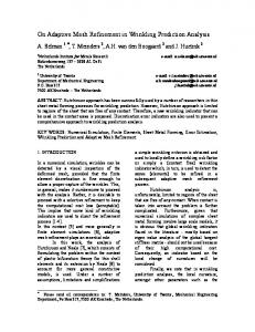
2.1 Hierarchy of nested grids We consider a set of nested dyadic grids. For simplicity, we only consider here embedded Cartesian grids. Information about structured nested grids in general coordinate system can however be found in [26]. Nested grid techniques have also been developed for unstructured grids [11, 27], where triangle or tetrahedral elements are considered. We note l = 0, 1, ...., L the grid level from the coarsest (l = 0) to the finest (l = L). At each grid level (l), we consider a partition of cells Vjl of the computational domain Ω. Vjl is considered as a control volume in the Finite-Volume terminology. The hierarchy of nested grids is based on a tree data structure which is used to encode the solution by means of the multiresolution analysis. Examples of embedded grids on a tree data structure are presented in figures (2.1, 2.2, and 2.3). The nodes are elements of the j= 1
j= 2
j = ....
j(l)= 2 j(l-1)-1
j(l)= 2 j(l-1)
j(l)= 2l
l = ....
j= 1
j= 3
j= 2
j= 4
l= 2
l= 1 j= 1
j= 2
j= 1
l= 0
Vj
l
Fig. 2.1: Dyadic tree data structure in 1D as a partition of the computational domain Ω.
tree, noted Λ (corresponding to black or red dots on Fig. 2.1), defined by the couple (j, l) corresponding to the position index (j) and the grid level (l). A control volume (Vjl ) is then associated to each node of the tree. The root (V10 ) denotes the basis of the tree. The leaves denote upper elements (nodes at the highest grid level), which have been enhanced in red in figure 2.1. In Ndim dimensions, a parent-cell at a level l (Vjl , in 1-D) has always l+1 in 1-D). If a node (j, l) ∈ Λ then the 2Ndim children-cells at the level l + 1 (V2jl+1 and V2j+1 parent-cell (j/2, l − 1) ∈ Λ and the children-cells (2j, l + 1) and (2j + 1, l + 1) ∈ Λ. The cell partition is dense in Ω, meaning that: ∩ ∪ Ω= Vjl with Vjl Vkl = 0 for j ̸= k; j, k ∈ Il , (2.3) j∈Il
where Il is the cell index set of Ω at grid level l. Moreover, we assume in a refinement
2.1. Hierarchy of nested grids
9
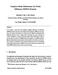
Fig. 2.2: Example of a 2D dyadic tree data structure as a partition of the computational domain Ω.
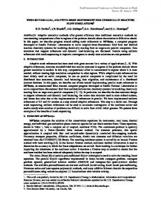
Fig. 2.3: Example of a 3D dyadic tree data structure as a partition of the computational domain Ω.
10
2. MULTIRESOLUTION PROCEDURE
process that between two consecutive grid-levels: ∪ Vjl = Vpl+1 ,
(2.4)
p∈Cjl
where Cjl is the index set of the chidren-cells of Vjl .
2.2 Mean value multiresolution: Finite-Volume approach The mean-value multiresolution is based on the cell-average value on each control volume at level l, expressed as follow, for instance in 3-dimensions: ∫ 1 l vi,j,k = l w(x, t) dx, (2.5) |Vi,j,k | Vi,j,k l where Vi,j,k := [2−l i,∫2−l (i + 1)] × [2−l j, 2−l (j + 1)] × [2−l k, 2−l (k + 1)] with i ∈ Z, j ∈ Z, l k ∈ Z and |Vi,j,k |=
dx is the measure of the control volume. l Vi,j,k
If we introduce a dual scaling function (φ) e based on the so-called box function: { 1 if x ∈ Vjl ; 1 φ elj = l χVjl (x) with χVjl = (2.6) |Vj | 0. elsewhere; the cell-average value of a scalar integrable function w ∈ L1 (Ω) can be interpreted as the inner product: vjl =< w, φ elj >Ω , (2.7) ∫ where the inner product is defined by < u, v >Ω := uv dx. Ω
The scaling function is normalized in L1 : following (2.6), ||φ el ||L1 = 1. Relations between cell-average values at different grid-levels (l) are based on the multiresolution analysis. Therefore, we define two operators, the projection and prediction operators, that allow us to represent a function by its cell-average values on a coarse grid (at grid level l − 1), knowing the function cell-average values on a finer grid (at grid-level l), and in the opposite direction, to predict cell-average values of the function on a fine grid (at grid-level l) from the function cell-average values known on a coarser one (at level l − 1). 2.2.1 Projection operator The projection operator (noted Pl+1→l ) allows one to compute the cell-average value of the solution at a grid node at level l from cell-average values of the solution known on children-nodes at grid level l + 1. As far as grids are nested, the projection operator
2.2. Mean value multiresolution: Finite-Volume approach
11
is exact and unique [11], given that cell-average values at two successive grid levels are related by: 1 ∑ l+1 l+1 (2.8) Pl+1→l : vjl = l |Vp | vp ; |Vj | l p∈Cj
where Cjl denotes the index set of the 2Ndim children-cells at grid level (l + 1) of the current cell Vjl . For 1-dimension, Cjl ∈ [2j, 2j + 1]. In such way, if the solution on leaves (at grid level l) is known, cell-average values can be calculated from grid level (l) down to the root-cell (l = 0). 2.2.2 Prediction operator ˆ l+1 of vl+1 . The prediction operator (noted Pl→l+1 ) maps vl to an approximate value v In contrast with the projection operator, there is an infinite number of choices for the definition of Pl→l+1 . Nevertheless, in order to be applicable and tractable in a graded tree structure, the prediction needs to be: • local ; this means that the interpolation stencil must contain the parent-cell and its nearest neighbors in each direction [11, 27]. • consistent with the projection operator, i.e. Pl+1→l ◦ Pl→l+1 = Id. In other words, ˆ l+1 must be conservative with respect to the average values the approximate value v on the coarser grid, vl : ∑ |Vpl+1 | vˆpl+1 |Vjl | vjl = (2.9) p∈Cjl
Let us notice that the linear property of the prediction operator is not necessarily required. Anyway, for simplicity of the numerical analysis, linear polynomial interpolation are often used to predict the approximated value vˆpl+1 . Information on non-linear operator can be found in Anr`andiga et al. [3]. As the approximation stencil contains the parent-cell and its nearest neighbors, we can consider centered linear polynomial interpolations of order o = 2 s + 1 of accuracy, based on the s-nearest neighboring cells to approximate vˆpl+1 : s ∑ ( l ) l+1 l l v − v , = v + ξ v ˆ q j+q j−q j 2j q=1 Pl→l+1 : (2.10) s ∑ ) ( l l+1 l l ξq vj+q − vj−q , vˆ2j+1 = vj − q=1
where ξq are coefficients of the linear polynomial interpolation of accuracy order o = 2 s+1, given in table 2.1 up to s = 5. Let us mention that when s = 0, the classical Haar basis is recovered. For s > 0, considering the child -cell Vjl , the stencil is: { } j l Rj = + q, |q| ≤ s; (l − 1) . (2.11) 2
12
2. MULTIRESOLUTION PROCEDURE
order (o) 1 3 5 7 9 11
s 0 1 2 3 4 5
ξ1 0 −1 8 −22 128 −201 1024 −3461 16384 −29011 131072
ξ2 0 0 3 128 11 256 949 16384 569 8192
ξ3 0 0 0 −5 1024 −185 16384 −4661 262144
ξ4 0 0 0 0 35 32768 49 16384
ξ5 0 0 0 0 0 −63 262144
Tab. 2.1: Coefficients of centered linear polynomial interpolations [19]
As far as Cartesian mesh is used, extension to multidimensional polynomial interpolations is easily obtained by a tensorial product of the 1-D operator [7, 30]. If we define the polynomial interpolation Qs as: s ( ) ∑ ( l ) l Qs j; v l = ξq vj+q − vj−q ,
(2.12)
q=1
the tensorial product of the polynomial interpolation in two dimensions, proposed by Bihari and Harten [7] reads: l+1 l l l vˆ2j+p,2k+q = vj,k + (−1)p Qs (j; v.,k ) + (−1)q Qs (k; vj,. ) − (−1)(p+q) Qs2 (j, k; vl ),
(2.13)
with p and q equal to either 0 or 1 depending on the child-cell considered. The polynomial Qs (2.12) is used in both directions and the operator Qs2 , derived from a tensorial product, reads: s s ∑ ( l ) ( ) ∑ l l l Qs2 j, k; vl = ξa ξb vj+a,k+b − vj−a,k+b − vj−a,k+b + vj−a,k−b , a=1
(2.14)
b=1
In the same way, polynomial interpolations are also extended to 3-dimensions by introducing a new operator Qs3 , also derived from a tensorial product, that reads: Qs3
s s s ∑ ∑ ( l ( ) ∑ l l l − vi−a,j+b,k+c − vi+a,j−b,k+c i, j, k; v = ξa ξb ξc vi+a,j+b,k+c a=1
b=1
c=1 l l l + vi−a,j+b,k−c + vi−a,j−b,k+c −vi+a,j+b,k−c ) l l , − vi−a,j−b,k−c +vi+a,j−b,k−c
(2.15)
Therefore, the 3D- polynomial interpolation reads: l+1 l l l l ) ) + (−1)r Qs (k; vi,j,. ) + (−1)q Qs (j; vi,.,k + (−1)p Qs (i; v.,j,k = vi,j,k vˆ2i+p,2j+q,2k+r (p+q) s l (p+r) s l −(−1) Q2 (i, j; v.,.,k ) − (−1) Q2 (i, k; v.,j,. ) (p+q+r) l (q+r) s Qs3 (i, j, k; vl ), −(−1) Q2 (j, k; vi,.,. ) + (−1) (2.16)
2.2. Mean value multiresolution: Finite-Volume approach
13
with p, q, and r equal to either 0 or 1 depending on the child-cell considered. When dealing with unstructured meshes based either on triangle or tetrahedral elements, it is much more delicate to derive multidimensional polynomial interpolations from the 1D-operator (2.10). Regarding unstructured meshes, detailed information can be found in Cohen et al. [11] and M. Postel [27]. 2.2.3 Multiresolution transform One can introduce a prediction error at a grid level l which is estimated by evaluating “details” (dlj ) defined as the difference between the numerical solution vjl and interpolated values vˆjl : (2.17) dlj = vjl − vˆjl . Following eq. (2.6 and 2.7), details can be interpreted as the inner product between e the solution (w) and a dual wavelet, noted ψ: dlj =< w, ψel > .
(2.18)
Following definitions of both the detail (2.17) and the cell average value in terms of the scaling function (2.7), ∑ < w, ψel >=< w, φ el > − cl−1 < w, φ el−1 >, (2.19) q q
the dual wavelet reads: ψel := φ el −
∑
cl−1 el−1 . q φ
(2.20)
q
cl−1 q
If we assume that prediction coefficients are uniformly estimated, the dual wavelet is e L1 ≤ C. normalized in L1 : ||ψ|| Thanks to the consistency assumption (2.8, 2.9, and 2.10), the sum of details (dlj ) on children-cells of a parent-cell is equal to zero [20]: ∑ |Vpl | dlp = 0. (2.21) p∈Cjl
Therefore, in Ndim dimensions, the knowledge of the 2Ndim children cell-averages of a given parent-cell is equivalent to the knowledge of the parent cell-average and 2Ndim − 1 details. Following A. Harten [20], if the function w has q −1 continuous derivatives and a jump discontinuity at its q-th derivative, then the detail behaves as: { (δxj )q [w(q) ] for 0 ≤ q ≤ o; dlj (v L ) ∼ (2.22) (δxj )o w(o) for q > o; where o is the accuracy order and [.] is the jump at the discontinuity. The main property required in the MR process is that the prediction approximation recovers o-th order of
14
2. MULTIRESOLUTION PROCEDURE
accuracy which is equivalent to say that it is exact for (o − 1)-th order polynomials. In such way, the details recover null values for smooth solutions with locally bounded o-th ∏ order derivatives [12]: i.e. ∀ u ∈ o−1 ((o − 1)-th order polynomials), then uj = uˆj and < u, ψel >= dl = 0.
(2.23)
The N first moments of the dual wavelet must then be null [12, 11, 27]. Moreover, as far as the solution is smooth, it was shown in [9, 13, 27] that details decay with a rate at least of 2−l : l dj ≤ C 2−l |v′ | ∞ l . (2.24) L (V ) j
Therefore, for smooth solutions, the higher the grid level is, the smaller the details are. On the other hand, details recover significantly high values in regions where singularities of the solution occur. Let us denote by Dl the vector of all details at a grid level l: { } Dl = dlj , 0 ≤ j ≤ Nl , with Nl = (2Ndim − 1) 2Ndim (l−1) for dyadic nested grids, we can observe that, following ( ) eq. (2.17 and 2.21), the knowledge of vl , Dl+1 is equivalent to the knowledge of v(l+1) : ( ) v(l+1) ↔ vl , Dl+1 .
(2.25)
Note that there is a one to one transformation between the two sets which have the same number of elements: Nl+1 = 2Ndim .(l+1) elements at grid level (l + 1) decomposed in 2Ndim .l values of vl plus (2Ndim − 1) 2Ndim .l details. Recursively on all L grid levels, one gets the so-called multiresolution transform [20] that maps the vector of the solution on the finest grid (vL ) to the solution on the root-cell plus all vectors of details from grid level l = 1 to the highest level (L): ( ) M : vL 7−→ v0 , D1 , . . . , DL = ML .
(2.26)
This multiresolution transform (M) is a one-to-one transformation between vL and ML , and in the case where the prediction operator Pl→l+1 is linear, it can be seen as a basis change, keeping the number of degrees of freedom unchanged: vL = M−1 ML ; ML = M vL
(2.27)
Encoding the solution known by its cell-average value on the finest grid is achieved by using the following Algorithm 1.
2.2. Mean value multiresolution: Finite-Volume approach
15
Algorithm 1 Encoding cell-average solution ML = M vL 1: Knowing the average values (vjL ) of the solution on the finest grid control volumes (VjL ); 2: for l = L − 1 down to 0 do 3: for j ∈ Il do 4: Calculation of cell averages vjl at grid level l by using the projection operator Pl+1→l (2.8): 2Ndim 1 ∑ l vj = l |V l+1 | vpl+1 ; (2.28) |Vj | p=1 p
5:
where p denotes indexes of the 2Ndim children-cells at grid level (l + 1) of the current cell Vjl . In fact, p ∈ [2j, 2j + 1] in each direction. Calculation of predicted values by using linear polynomial interpolations (2.12, 2.14 or 2.15): ˆ l+1 = Pl→l+1 vl v
6:
ˆ l+1 by using (2.17): Calculation of details between vl+1 and v l+1 l+1 dl+1 ˆ2j 2j = v2j − v
7:
8: 9: 10:
{ } Ndim Store the set of details in the vector Dl+1 = dl+1 − 1) 2Ndim .l . p , 0 ≤ p ≤ (2 If needed, the last detail can be computed by consistency relations eq. (2.21). Encode the solution by replacing the cell-average values on the fine grid, vl+1 , by the cell-average values on the coarser grid plus the details, (vl , Dl+1 ); end for end for 2(L+1).Ndim − 1 Considering a complete tree data structure having nodes among its 2Ndim − 1 2L.Ndim leaves, the cell-average function v is now encoded by using the new data format with one cell-average value on the root-cell and 2L.Ndim − 1 details: ML = ( 0 1 ) v , D , . . . , DL .
In the opposite way, decoding the solution known by its cell-average values on the coarsest grid and the set of details is obtained through the use of the following Algorithm 2.
16
2. MULTIRESOLUTION PROCEDURE
Algorithm 2 Decoding cell-average solution vL = M−1 ML 1: We here assume that the solution w is known by its cell-average values (vj0 ) on the ( ) control volumes (Vj0 ) of the coarsest grid and the set of details D1 , . . . , DL ; 2: for l = 0 up to L − 1 do 3: for j ∈ Il do 4: Knowing the cell-average value, vjl , of the current cell Vjl and the local details, l l Ndim dl+1 children-cells of Vjl ; p , p ∈ Cj , where Cj is the index set of the 2 5: Interpolate vˆpl+1 , p ∈ Cjl by using the centered linear polynomial interpolations Pl→l+1 (2.10, 2.13 or 2.16); 6: Calculate cell-average values vpl+1 , p ∈ Cjl at grid level l + 1 by (2.17): l vpl+1 = vˆpl+1 + dl+1 p , p ∈ Cj ;
(2.29)
In fact, 2Ndim − 1 values of the cell-average is computed through eq.( 2.29). The last value is computed by consistency relations eq. (2.9, 2.21). For instance, in one dimension, we have: l+1 l+1 v2k = vˆ2k + dl+1 2k ; l |Vj | l+1 l+1 v2k+1 = vjl − v2k ; l+1 |V2k+1 |
(2.30) (2.31)
Decode the solution replacing (vl , Dl+1 ) by vl+1 ; 8: end for 9: end for 10: The solution w is now known by its 2L.Ndim cell-average values vjL , j ∈ IL on the finest grid. 7:
The new data format is however more convenient for data compression because detail magnitudes are zero when solutions have locally bounded o-th order derivatives and decay with the grid level (2l for smooth solutions). Nevertheless, to be competitive for computations, the multiresolution transform should not increase the computational complexity related to the number of floating point operations required by the algorithm. In order to decrease the computational complexity, one of the solutions is to adapt locally the mesh, considering the behavior of the solution, which should yield lower CPU time and memory requirements.
2.3 Thresholding and compression Indicator functions are needed to locate regions where the solution requires a mesh refinement for capturing small scale structures. Here, assuming that the multiresolution basis 2.26 is stable [11], this indicator is based on the details because they decay with the
2.4. Building of a graded tree
17
grid level for smooth solutions and recover sufficiently large values in singular regions. The idea is to retain only the details whose values are greater than a threshold parameter (εl ) on each grid level (l) and set the others to zero. In practice, when we deal with systems of equations, the measure of the details is computed through the L1 -norm of the vector dl , which seems natural for conservation law problems. The threshold operation (T ) is then obtained by taking into account a measure of details scaled by global maximum, following: |dlj |L1 < εl =⇒ dlj = 0; if maxj |dlj | (2.32) Tεl (d) = otherwise dlj ∈ Dl . Therefore, the computational mesh is formed by leaves such that the normalized L1 -norm of their details is greater than εl . In order to obtain data compression, leaves with their details set to zero are discarded from the tree structure. Therefore, we define the index and grid level set (Λε ) of nodes that belong to the compressed tree data structure: { } Λεl = (j, l) s.t. |dlj | ≥ εl (2.33) We can then define the multiresolution (MR) approximation operator (AΛεl ) that maps the function (the finite-volume solution for conservation law) on the unique finest grid (vL ) to the function evaluated on the refined nested grids: AΛεl := M−1 Tεl M
(2.34)
Let us remark that the MR operator AΛεl is non linear since it depends on the solution vL through the threshold procedure (2.33). We can then compute the perturbation error defined as the difference between the finite-volume solution evaluated on the finest grid and the solution obtained on the refined grid by using the multiresolution algorithm. This perturbation error intrinsic to the MR algorithm, recovers the following form [11, 27]: ∑ ∥vL − AΛεl vL ∥ = C |dl | 2−Ndim l (2.35) |dl | root(i, j, k) call evaluation(current) enddo enddo enddo where type(child cell), dimension(number root(1),number root(2),number root(3)) :: root type(cell) :: current Into a general routine, in this case evaluation as an example, the recursive scheme is presented in the following for evaluating a function only on leaves: recursive subroutine evaluation(current) if (.not.associated(current%children(1))) then !
we are on a leaf,
current%u = .... else do n = 1, 2**Ndim call evaluation(current%children(n)) enddo endif end subroutine evaluation In this recursive way, we are able to locate the leaves considering the states of the pointers that link cells at different levels. The same kind of procedure is conducted in the opposite direction, from the leaves towards the roots, or when the prediction stencil of a given cell needs to be located, for example. This could be achieved using the following example where the value of a function is known on leaves and we would like to propagate the function down to the root:
32
3. ALGORITHMS AND CODE STRUCTURE
recursive subroutine evaluation(current) if (.not.associated(current%children(1))) then !
we are on a leaf, nothing is done
else do n = 1, 2**Ndim call evaluation(current%children(n)) enddo current%u = .... endif end subroutine evaluation Possibly, other parameters as the index of the cell or the pointers to the neighbors, are also taken into consideration during the research. It is clear that more performing navigation schemes yield certainly more efficient strategies.
4. TEST-CASES
In this part, we apply the MR procedure to several classical test-cases to illustrate the influence of the MR parameters on the performance of the method. Hence, the first example is devoted to check the influence of the threshold value (ε) and the stencil width (s) on the accuracy as well as on the compression rate in the memory use. This first testcase can be handled in 1D, 2D or 3D Cartesian geometries. Next examples are devoted to the solution of PDE, either for the solution of hyperbolic equations or nonlinear reactiondiffusion problems.
4.1 Multiresolution on 1D-functions: some examples This section illustrates the compression of functions on dyadic grids. Four functions with different smoothness are tested: ( ) f1 (x) = exp −50 x2 (4.1) √ ( π ) f2 (x) = 1. − sin x (4.2) 2 f3 (x) = tanh (50. x) (4.3) f4 (x) = 0.5 − |x|
(4.4)
where x ∈ [0, 1.]. A code written in Fortran95 is provided to check the influence of some MR parameters, namely the influence of the threshold value (ε) and the stencil width (s) of the prediction operator which gives the accuracy order (o = 2s + 1) as we have already seen in (2.10. This code, which its main program is named MR function.f90, is based on a dyadic tree structure and derived type variables. Figures 4.1, 4.2, 4.3, and 4.4 illustrate the MR coding of the four functions (equations 4.1, 4.2, 4.3, and 4.4). We ran the code using a domain extent x ∈ [−1, +1] with a width of the approximation polynomial s = 1 and a threshold value ε = 10−2 . The threshold parameter (ε) has a crucial influence on the error introduced by the MR procedure [11]; therefore, it is important to check how MR solutions converge with ε. On figure 4.5, we plotted the perturbation error in L1 -norm, calculated as the difference between the exact solution and the MR solution for several ε values, obtained on 10 grid levels. The perturbation error almost recovers a linear fit versus ε which is in complete agreement with the heuristic MR approach (2.39) from Harten’s work [20].
4. TEST-CASES
1
0.001
8
0.8
0.0008
6
0.6
|| Error ||L1
10
0.0006
a
grid-level
34
4
0.4
0.0004
2
0.2
0.0002
0 -1
-0.5
0
0.5
0 -1
1
-0.5
x
0
0.5
0 -1
1
-0.5
0
0.5
1
x
x
1
0.001
8
0.8
0.0008
6
0.6
|| Error ||L1
10
0.0006
a
grid-level
Fig. 4.1: Analysis of the function y = f1 (x), with a reconstruction accuracy o = 3 and a threshold value ε = 10−2 : on the left, grid level and locations of leaves; in the center, the reconstructed function on leaves, and on the right, errors (in the L1 norm) compared to the exact solution.
4
0.4
0.0004
2
0.2
0.0002
0 -1
-0.5
0
0.5
0 -1
1
-0.5
x
0
0.5
0 -1
1
-0.5
0
0.5
1
x
x
1
0.001
8
0.8
0.0008
6
0.6
|| Error ||L1
10
0.0006
a
grid-level
Fig. 4.2: Analysis of the function y = f2 (x), with a reconstruction accuracy o = 3 and a threshold value ε = 10−2 : on the left, grid level and locations of leaves; in the center, the reconstructed function on leaves, and on the right, errors (in the L1 norm) compared to the exact solution.
4
0.4
0.0004
2
0.2
0.0002
0 -1
-0.5
0
x
0.5
1
0 -1
-0.5
0
x
0.5
1
0 -1
-0.5
0
0.5
1
x
Fig. 4.3: Analysis of the function y = f3 (x), with a reconstruction accuracy o = 3 and a threshold value ε = 10−2 : on the left, grid level and locations of leaves; in the center, the reconstructed function on leaves, and on the right, errors (in the L1 norm) compared to the exact solution.
4.1. Multiresolution on 1D-functions: some examples
1E-06
10
8E-07
0.4
6E-07
8
|| Error ||L1
0.2 6
a
grid-level
35
0
4E-07 2E-07 0
-2E-07
4
-4E-07
-0.2
-6E-07
2
-8E-07
-0.4 0 -1
-0.5
0
0.5
1
-1
-0.5
x
0
0.5
-1E-06 -1
1
-0.5
0
0.5
1
x
x
Fig. 4.4: Analysis of the function y = f4 (x), with a reconstruction accuracy o = 3 and a threshold value ε = 10−2 : on the left, grid level and locations of leaves; in the center, the reconstructed function on leaves, and on the right, errors (in the L1 norm) compared to the exact solution.
10-2
|| v - v
MR
||
10-6
10-8
0.8 0.7
10-10
10
-12
10
-14
10
-16
s=1 s=2 s=3
0.9
Memory Usage
10-4
1 L∞: s=1 L1: s=1 2 L : s=1 L∞: s=2 1 L : s=2 L2: s=2 L∞: s=3 1 L : s=3 2 L : s=3 ε
0.6 0.5 0.4 0.3 0.2 0.1
10-13
10-11
10-9
10-7
ε
10-5
10-3
10-1
0 10-13
10-11
10-9
10-7
ε
10-5
10-3
10-1
Fig. 4.5: Capability of the MR procedure: On the left, L∞ , L1 and L2 -norms of the pertubation error versus the threshold parameter (ε) obtained on 10 grid levels (i.e. the finest grid has 1024 grid points); on the right, the memory use compared to the finest grid.
36
4. TEST-CASES
4.1.1 Implementing adaptive grid The structure of a grid cell, as previously mentioned (see § 3.2), is defined in a module, named mod structure.f90. Basic parameters of the MR algorithm are defined in a common file, named mod common.f90. Algorithm 7 MR functions 1: Input parameters (geometrical and MR parameters) are read from a data file (named don function.dat) with routine: lect don.f90. 2: The tree structure is built and linked, in recursive procedures: • creating and linking nodes in the tree: chainage.f90; • linking roots if we employ a tree forest: support racine.f90; • and linking support chainage support.f90.
corresponding
to
the
approximation
stencil:
3: The initial solution is prescribed on the leaves of the tree: init sol.f90
This routine is in the module mod fonction.f90, where the various functions are defined. 4: The MR algorithm is based on several recursive routines devoted to: • Encoding the average value at cell centers, from leaves down to the root: encoding moy.f90; • Encoding details, from leaves down to the root: encoding det.f90; • Thresholding the solution with respect to ε value: seuillage.f90; • Building the graduate tree: graduation.f90 and graduation local.f90; • Decoding the average value at the cell centers, from the root up to leaves: decoding moy.f90; • Discarding undesirable leaves: elagage.f90; • Linking cells for the chainage support.f90;
approximation
stencil
in
the
tree
structure:
12: Listing and printing leaves: liste feuille.f90 and print leaves.f90, respectively.
All these routines are included in a module named mod arbre.f90. By means of the make command, which reads the Makefile provided, the compilation builds an executable, named mr function.x.
4.1. Multiresolution on 1D-functions: some examples
37
Input parameters are read in a data file, named don function.dat, that gathers all parameters that can be modified in order to check their influence. This file is structured as follow: • num funct ∈ [1, 4]: the function number, corresponding to functions (4.1), (4.2), (4.3), and (4.4), respectively; • lim deb, lim fin: Left and right limits of the domain; • niv max : the maximum grid level; • niv min: the minimum grid level; • s: the stencil width of the prediction approximation; • ε: the threshold value. Let us notice that the maximum number of points used on the finest grid is: N = . 2 At the exit, two files are generated: niv max
• a file containing the solution evaluated on leaves of the tree. It is named: Tree funct(num funct ) niv(niv max ) L1s(s ) eps(ε).dat, where (num funct) is the value of the function number, (niv max ) is the value of the maximum grid level, (s) is the value of the stencil width, and (ε) is the threshold value. The five columns of this file correspond to: the leaf coordinate, the grid spacing, the leaf level, the value of the function on the leaf and the error compared to the exact solution evaluated on the leaf. • a file containing errors with respect to the exact solution. It is named: Err funct(num funct ) niv(niv max ) L1s(s ).dat. Results are saved in columns: Four columns corresponding to: the threshold value, ε; the L∞ norm, the L1 norm, the L2 norm of errors compared to the exact solution, and compression rate Nleaves /2niv max . Finally, in order to run the program after compiling, we just need to type: ./mr function.x However, a script shell (named function.sh) is also provided to run the executable several times for different threshold values (ε). The threshold value starts at ε = 10−1 and ends at ε = 10−12 with a step of 10−1 . Errors for these different ε values are collected in the file Err funct(num funct ) niv(niv max ) L1s(s ).dat so that they could be plotted
38
4. TEST-CASES
versus the threshold parameter (with “gnuplot”, for instance) to check the order of the method. Using this executable, your can: 1. Check the influence of the threshold parameter (ε) for all the functions prescribed in the code. • Prescribe the number of a function you would like to check; • Prescribe the number of grid levels, 10 for instance; • Prescribe the width of the approximation stencil, s = 1, for instance; • Run the code (./mr function.x) with the script shell ./function.sh to let evolve ε from 10−1 to 10−12 ; • Plot errors compared to the exact solution for several threshold values, versus ε by using gnuplot, for instance. (Errors are recorded in Err funct(num funct ) niv(niv max ) L1s(s ).dat • You could also plot the compression rate of memory use versus ε. 2. Check the influence of the width of the approximation stencil (s) for the above described functions. • Prescribe the width of the approximation stencil; • Run the code (./mr function.x) with the script shell ./function.sh to let evolve ε from 10−1 to 10−12 ; • Plot errors compared to the exact solution versus ε. • You could also plot the compression rate of memory use versus ε. 3. Check the influence of the constraint (2.41 in Algorithm-5) to foresee discontinuity by modifying the variable precis (which is originally set to 2 s − 1) in the routine seuillage.f90. Recompile the executable and proceed as above to check the influence on the accuracy or the memory compression. 4. Prescribe your favorite functions in the module mod fonction.f90. Recompile and proceed as above to check the influence of the MR parameters on the accuracy and memory use. 5. Modify the number of dimensions of the problem (Ndim ) in the module file mod common.f90. Be sure that functions are well defined for multi-dimension evaluation. Recompile and proceed as above to check the influence of the MR parameters on the accuracy and memory use.
4.2. Hyperbolic equations: scalar advection
39
4.2 Hyperbolic equations: scalar advection We here focus on the solution u(x, t) of the linear scalar transport equation: ∂u ∂t + ∇ · f (u) = 0, in Ω, u(0, t) = u(1, t), on ∂Ω, u(x, 0) = u0 (x),
(4.5)
with f (u) = a u, a being the velocity which is independent of the solution u(x, t). We propose to solve this transport equation by using MR algorithm in both 1D and 2D Cartesian grids. 4.2.1 1D scalar advection Assuming that the speed is constant, the equation reads: ∂u ∂u +a = 0. ∂t ∂x
(4.6)
with periodic boundary conditions. The analytical solution of this equation is the convection at the speed a of the initial solution: u(x, t) = u0 (x − a t). (4.7) In this example, we prescribe the initial solution at: u(x, 0) = −Vlef t sin (2. π x) ; x ∈ [0, 1],
(4.8)
where Vlef t is an input value. 4.2.1.1 Numerical method and results This equation is solved using a One-Step scheme developed in Daru & Tenaud [15] based on a Lax-Wendroff approximation [23]. This scheme is constructed in the scalar case by correcting the error terms of the successive modified equations, to yield one additional order of accuracy at each level. For stability reasons, the error term, involving highest degree derivatives at each level, is discretized using upwind formulae for odd derivatives and centered formulae for even derivatives. In this way, one obtains a recurrence relation to construct schemes with arbitrary order of accuracy in time and space. This scheme (named OS7) is time-space coupled, with 7th-order time and space accuracy. It was shown Daru & Tenaud [16] that OS7 is at least six times more efficient in CPU time performance than the well known method of lines using a Runge-Kutta time integration and WENO schemes for space discretizations that recover the same accuracy.
40
4. TEST-CASES
To illustrate this scheme, let us introduce the discrete form of equation 4.7: un+1 = Ej unj = unj − j
δt lw lw (F − Fj−1/2 ), δx j+1/2
(4.9)
lw where Fj+1/2 is the Lax-Wendroff numerical flux:
lw Fj+1/2 = fjn +
(1 − ν) n (fj+1 − fjn ), 2
(4.10)
δt . The modified equation for this scheme reads: and ν is the local CFL number ν = a δx
ut + f (u)x = a
δx2 2 (ν − 1)uxxx . 6
(4.11)
By subtracting from the Lax-Wendroff scheme an upwind term formed by discretizing the right hand side of (4.11), one obtains the classical third order upwind-biased scheme with a numerical flux which can be written: 3 Fj+1/2 = fjn +
1+ν n (1 − ν) n n (fj+1 − fjn − (fj+1 − 2fjn + fj−1 )). 2 3
(4.12)
For convenience, this numerical flux can be recast in the generic form: o Fj+1/2 = fjn + Φoj+1/2
(1 − ν) n (fj+1 − fjn ). 2
(4.13)
So, the discretization of equation 4.7 that defines the operator (Ej ) is the following: ujn+1 = Ej unj = unj −
δt o o (Fj+1/2 − Fj−1/2 ), δx
(4.14)
Thus, the o-th order scheme is expressed in the usual form of a second order flux limiter scheme, and the Φoj+1/2 function plays the role of an accuracy function that drives the o-th order of accuracy of the scheme. Following such successive corrections of the higher order error terms, one can construct schemes of arbitrarily high o-th order of accuracy. In this way we can obtain the function Φo corresponding to a o-th order (in time and space) scheme: We performed the successive derivations of the modified equations up to sixth un −un j−1 order. By defining rj+1/2 = ujn −u n , Φ functions up the the seventh order of accuracy are j+1 j provided here: (4.15)
4.2. Hyperbolic equations: scalar advection
41
1+ν (1 − rj+1/2 ), 3 1+ν ν−2 = Φ3j+1/2 + · (1 − 2 rj+1/2 + rj+1/2 rj−1/2 ) 3 4 1+ν ν−2 ν−3 = Φ4j+1/2 − · · · 3 4 5 ( ) 1 − 3 + 3 rj+1/2 − rj+1/2 rj−1/2 rj+3/2
Φ3j+1/2 = 1 − Φ4j+1/2 Φ5j+1/2
1+ν ν−2 ν−3 ν+2 Φ6j+1/2 = Φ5j+1/2 + · · · · 3 4 5 6 ( ) 1 4 − + 6 − 4 rj+1/2 + rj+1/2 rj−1/2 rj+3/2 rj+5/2 rj+3/2
(4.16)
1+ν ν−2 ν−3 ν+2 ν+3 Φ7j+1/2 = Φ6j+1/2 − · · · · · 3 4 5 6 7 ( 1 5 − + 10 − 10 rj+1/2 + 5 rj+1/2 rj−1/2 rj+3/2 rj+5/2 rj+3/2 ) −rj+1/2 rj−1/2 rj−3/2 Let us emphasize that the numerical schemes constructed in this way always have the same order of accuracy in time and space. Here we use a stencil of only nine points to get a seventh order scheme relative to both time and space. This kind of scheme has the property, which seems desirable, of giving the exact solution if the CFL number is equal to 1, though the scheme has a classical CFL stability condition; 0 ≤ ν ≤ 1. We performed integration of equation (4.6) by using the OS7 scheme, assuming that the characteristic speed a = 1. Figure 4.6 illustrates the mesh adaptation by the MR algorithm for the solution computed at several times on a mesh with 7 grid-levels. These solutions are obtained by using a domain extent x ∈ [−1, +1] with a width of the approximation polynomial s = 1 and a threshold value ε = 10−2 . 4.2.1.2 Implementing adaptive grid We consider here the propagation of an initial function with a constant speed, using a grid adaptivity based on a MR technique. The structure of the code is the one described in the Algorithm-6 by using the evolution operator defined in equation(4.14) based on a one-step 7-th order accurate scheme in time and space [15, 16]. To run the code that solves this problem using MR technique, we just need to type: ./mr scalar1D.x Input parameters are read in a data file, named don scalar1D.dat, that gathers all parameters that can be modified in order to check their influence. This file is structured as follow:
42
4. TEST-CASES
1
0.01
0.008
|| Error ||L1
0.5
a
0.006
0
0.004
-0.5 0.002
-1 -1
-0.5
0
0.5
0
1
-0.5
x
(a)
0
0.5
1
0.5
1
0.5
1
0.5
1
0.5
1
x
1
0.01
0.008
|| Error ||L1
0.5
a
0.006
0
0.004
-0.5 0.002
-1 -1
-0.5
0
0.5
0
1
-0.5
x
(b)
0
x
1
0.01
0.008
|| Error ||L1
0.5
a
0.006
0
0.004
-0.5 0.002
-1 -1
-0.5
0
0.5
0
1
-0.5
x
(c)
0
x
1
0.01
0.008
|| Error ||L1
0.5
a
0.006
0
0.004
-0.5 0.002
-1 -1
-0.5
0
0.5
0
1
-0.5
x
(d)
0
x
1
0.01
0.008
|| Error ||L1
0.5
a
0.006
0
0.004
-0.5 0.002
-1 -1
(e)
-0.5
0
x
0.5
1
0
-0.5
0
x
Fig. 4.6: Scalar advection in 1D, with a reconstruction accuracy o = 3, (s = 1) and a threshold value ε = 10−2 : the initial solution obtained on 7 grid levels (N = 128 grid points for the finest grid), is convected with a unit velocity a = 1. From top to the bottom, the solution is plotted at (a) the initial time and at several recorded times: (b) t = 0.5, (c)
4.2. Hyperbolic equations: scalar advection
43
• lim deb, lim fin: Left and right limits of the domain; • caltype deb, caltype fin: Left and right boundary conditions at limits of the domain; caltype must take one of the following values:
• caltype = -1 ⇒ symmetry condition • caltype = 0 ⇒ homogeneous Neumann condition • caltype = 1 ⇒ homogeneous Dirichlet condition • caltype = 2 ⇒ periodic condition • Vlef t : magnitude of the initial condition as defined in (4.8); • Vright : magnitude of the initial condition , if needed; • CFL: CFL number, 0 ≤ CF L ≤ 1; • Nmax : number of time steps; • niv max : the maximum grid level; • niv min: the minimum grid level; • s: the stencil width of the prediction approximation; • ε: the threshold value. • t min: initial recorded time; • δtsave : time step for the recorded time; • t final : final time at which the simulation stops. Let us notice that the maximum number of points used on the finest grid is: N = 2 . At the exit, the solution evaluated on the leaves of the tree is saved in a file named: Tree t(time save ) niv(niv max ) L1s(s ) eps(ε).dat, where (time save) is the time value at which the solution is saved, (niv max ) is the value of the maximum grid level, (s) is the value of the stencil width, and (ε) is the threshold value. The five columns of this file correspond to: the leaf coordinate, the grid niv max
44
4. TEST-CASES
spacing, the leaf level, the value of the solution on the leaf and the error compared to the exact solution evaluated on the leaf. Using the executable ./mr scalar1D.x, your can: 1. Check the influence of the maximum grid level (niv max).
2. Check the influence of the threshold parameter (ε).
3. Check the influence of the width of the approximation stencil (s) for the above described functions. We know that the perturbation (MR) error is linear versus the threshold parameter ε. To recover this behavior, you must first run the code with ε = 0. to get the solution on the finest grid everywhere. You must secondly save the solution for different ε values. The perturbation error is defined as the difference between the finite-volume solution evaluated everywhere on the finest grid and the solution obtained on the refined grid for different ε values by using the MR algorithm. Since the solution on an adapted grid is not evaluated at the same locations than on the finest grid, one needs to propagate the solution evaluated on the adapted grid toward the finest grid, assuming that details = 0. and using the approximation stencil with the prescribed width (s). This could be accomplished by W1 W2 W3 W4 W5
V1
U1
V2
U2
V3
V4
U3
V5
U4
U5
Fig. 4.7: Local reconstruction by mean value using approximation polynomial based on s = 1 nearest points.
means of a linear function applied on 5 centered values, as it is (Fig. 4.7): 1 − 18 1 0 8 1 + 8 1 − 81 0 1 1 V = Av U with Av = 0 −8 1 8 1 1 0 + 1 − 8 8 1 0 0 −8 1
illustrated in the scheme 0 0 0 0 1 8
(4.17)
4.2. Hyperbolic equations: scalar advection
45
• Could you write down a routine that propagates the solution known on the adapted grid towards the finest grid; • Calculate the perturbation errors in the L1 -norm; • Then, plot the perturbation errors versus the threshold parameter (ε) to show that this error recovers a linear fit with ε. • To study the efficiency of the algorithm in terms of memory compression, you could also plot the compression rate of memory use versus ε. 4.2.2 2D scalar advection In that case, the equation reads: ∂u + a · ∇u = 0. ∂t
(4.18)
with periodic boundary conditions and the initial condition u(x, t) = u0 (x). Here a is a vector with two components that are independent of the solution u(x, t) In the present example, the computational domain is (x × y) ∈ [−1, 1] × [−1, 1]. We consider the transport of a cylindrical spot that is initially located at x0 = 0.5, y0 = 0.: u0 (x, y) = (1. − C) Vright + C Vlef t , {
where C=
1. 0.
(4.19)
√ if (x − x0 )2 + (y − y0 )2 ≤ r02 , otherwise
with r0 = 0.25 The transport velocity vector a is prescribed at a cylindrical flow: a(1) = −y, a(2) = +x.
(4.20)
4.2.2.1 Numerical method and results This equation is solved using a One-Step scheme (OS7). The extension in the multidimensional case is delicate as far as a one-step approach is used. In fact, we need to consider cross derivative terms that appear in the second and higher order terms. The simplest way to avoid the problem of cross derivatives and to recover the good properties of the one-dimensional scheme is to use a Strang directional splitting strategy [24, 34], which is unfortunately only second order accurate. While the order of accuracy is lowered compared to the tensorial multistage approach, the OSMP scheme with the Strang algorithm gives results with very small errors at lower cost [15].
46
4. TEST-CASES
In two dimensions, the splitting of the system of equations (4.18) is written: wjn+2 = Lδx Lδy Lδy Lδx wjn .
(4.21)
Here Lδx and Lδy are discrete approximations of operators in each space direction. When directional operators do not commute, the second order accuracy is recovered every two time steps with however the symmetric property of the solution [15]. We then performed the integration of equation (4.18) using the OS7 scheme developed in Daru & Tenaud [15], already presented above. Figure 4.8 illustrates the mesh adaptation by the MR algorithm for the solution computed at several times with 7 grid levels (N = 128 × 128 for the finest grid). These solutions are obtained by using a width of the approximation polynomial s = 1 and a threshold value ε = 10−3 . 4.2.2.2 Implementing adaptive grid We consider here the propagation of an initial cylindrical spot with constant speed, using a grid adaptivity based on a MR technique. The structure of the code is the one described in the Algorithm-6 by using the evolution operator defined in equation(4.21) based on a onestep 7-th order accurate scheme in time and space and a directional splitting procedure [15, 16]. To run the code that solves this problem using MR technique, we just need to type: ./mr scalar2D.x Input parameters are read in a data file, named don scalar2D.dat, that gathers all parameters that can be modified in order to check their influence. This file is structured as follow: • lim deb(1), lim fin(1): Left and right limits of the domain; • caltype deb(1), caltype fin(1): Left and right boundary conditions at limits of the domain;
• lim deb(2), lim fin(2): Bottom and top limits of the domain; • caltype deb(2), caltype fin(2): Bottom and top boundary conditions at limits of the domain; caltype must take one of the following values:
• caltype = -1 ⇒ symmetry condition
4.2. Hyperbolic equations: scalar advection
t=1
1
1
0.5
0.5
0
0
y
y
t=0
-0.5
-1 -1
-0.5
-0.5
0
0.5
-1 -1
1
-0.5
0
x
0.5
0.5
0
0
-0.5
0.5
1
0.5
1
-0.5
-0.5
0
0.5
-1 -1
1
-0.5
0
x
x
t=4
t=5
1
1
0.5
0.5
0
0
y
y
1
t=3 1
y
y
t=2
-0.5
-1 -1
0.5
x
1
-1 -1
47
-0.5
-0.5
0
0.5
1
x
-1 -1
-0.5
0
x
t=6 1
y
0.5
0
-0.5
-1 -1
-0.5
0
0.5
1
x
Fig. 4.8: Scalar advection in 2D, with a reconstruction accuracy o = 3, (s = 1) and a threshold value ε = 10−3 : the initial solution is convected with a cylindrical vortex with a speed √ magnitude a(1)2 + a(2)2 = 0.5. The solution obtained by using 7 grid-levels, is plotted at the initial time and every dimensionless time unit.
48
4. TEST-CASES
• caltype = 0 ⇒ homogeneous Neumann condition • caltype = 1 ⇒ homogeneous Dirichlet condition • caltype = 2 ⇒ periodic condition • Vlef t : magnitude of the initial solution inside the cylindrical spot as defined in (4.19); • Vright : magnitude of the initial solution outside the cylindrical spot as defined in (4.19); • CFL: CFL number, 0 ≤ CF L ≤ 1; • Nmax : number of time steps; • niv max : the maximum grid level; • niv min: the minimum grid level; • s: the stencil width of the prediction approximation; • ε: the threshold value. • t min: initial recorded time; • δt save: time step for the recorded time; • t final : final time at which the simulation stops. Let us notice that the maximum number of points used on the finest grid is: N = 2 × 2niv max . At the exit, the solution evaluated on the leaves of the tree is saved in a file named: Tree t(time save ) niv(niv max ) L1s(s ) eps(ε).dat, where (time save) is the time value at which the solution is saved, (niv max ) is the value of the maximum grid level, (s) is the value of the stencil width, and (ε) is the threshold value. The solution is written in a finite-element format: niv max
• Corner coordinates of leaves are first listed; • For each leaf, a list of connectivity between leaf corners is secondly printed; • For each leaf, values of the solution at center of the leaf are finally printed. Using the executable ./mr scalar2D.x, your can:
4.3. Hyperbolic equations: non-linear cases
49
1. Check the influence of the maximum grid level (niv max).
2. Check the influence of the threshold parameter (ε).
3. Check the influence of the width of the approximation stencil (s) for the above described functions.
If you would like to compute the perturbation error, you need to propagate the solution evaluated on leaves of the adapted grid toward the finest grid and calculate the difference between the finite-volume solution with ε = 0 and the solution obtained on the adapted grid for different ε values.
4.3 Hyperbolic equations: non-linear cases We here focus on the solution u(x, t) of the 1D burger equation: ∂u ∂t + ∇ · f (u) = 0, in Ω, u(0, t) = u(1, t), on ∂Ω, u(x, 0) = u0 (x),
(4.22)
1 with f (u) = u2 . We propose to solve this non linear transport equation by using MR 2 algorithm. Here, we consider the initial solution: u(x, 0) = −Vlef t sin (2. π x) ; x ∈ [0, 1],
(4.23)
where Vlef t is an input value. 4.3.1 Numerical method and results This equation is solved using a One-Step scheme. We know that non linearity can lead to discontinuity creations after finite times, even if the solution is initially smooth. To prevent spurious oscillations due to Gibbs phenomenon in the vicinity of strong gradient regions, an ad hoc limiting process must be employed. Total Variation Diminishing (TVD) schemes are generally considered to be well suited for the capture of sharp discontinuities without oscillations. Nevertheless, TVD constraints are known to clip the extrema, which appears as a serious drawback in a limiting procedure. To avoid this loss of accuracy near extrema, it is necessary to satisfy the Monotonicity Preserving (MP) criteria, introduced by Suresh and Huynh [35], that enlarge the TVD intervals to provide room for the numerical flux
50
4. TEST-CASES
to maintain an accurate value. Daru and Tenaud [15] derived a Monotonicity Preserving version of the present scheme (named OSMP) that preserves accuracy near extrema. In particular, the original MP constraints of Suresh and Huynh [35] has been recasted in the TVD framework without CFL restriction to generalize the MP conditions in terms of flux limiting. The MP conditions that preserve accuracy can be expressed directly as constraints on Φo functions [15] (see equations 4.13 and 4.14). The MP constraints can be found in [15, 16]. P By taking the limiting function Φo−M in (4.13), the resulting scheme will be highk order accurate almost everywhere, except around discontinuities where it becomes first order accurate, which is the case for all TVD schemes. Let us note that the essential difference is that MP constraints act for non-monotone data and so far are TVD for monotone data such that the scheme is not oscillatory around discontinuities. We then performed the integration of equation (4.22) using the limited OSMP7 scheme developed in Daru & Tenaud [15]. Figure 4.9 illustrates the mesh adaptation by the MR algorithm for the solution computed at several times with 10 grid levels (N = 1024 grid points on the finest grid). These solutions are obtained by using a width of the approximation polynomial s = 1 and a threshold value ε = 10−2 . We can see (Fig. 4.9) that a shock like structure is created from a dimensionless time close to t = 0.4. In that region, the MR method foresees the discontinuity by refining the mesh up to the highest grid level (l = 10). The solution is finally represented over 5 grid-levels (from l = 6 to 10). 4.3.1.1 Implementing adaptive grid The structure of the code is the one described in the Algorithm-6 by using the evolution operator Ej based on a one-step 7-th order Monotonicity-Preserving (OSMP7) accurate scheme [15, 16]. To run the code that solves this problem using MR technique, we just need to type: ./mr burger1D.x Input parameters are read in a data file, named don burger1D.dat, that gathers all parameters that can be modified in order to check their influence. This file is structured as follow: • lim deb(1), lim fin(1): Left and right limits of the domain; • caltype deb(1), caltype fin(1): Left and right boundary conditions at limits of the domain; caltype must take one of the following values:
1
9
0.8
8
0.6
7
0.4
6
0.2
5
-0.2
3
-0.4
2
-0.6
1
-0.8 -0.5
0
0.5
-1 -1
1
-0.5
t = 0.1
10
1
9
0.8
8
0.6
7
0.4
6
0.2
5
0
4
-0.2
3
-0.4
2
-0.6
1
-0.8 -0.5
0
0.5
-1 -1
1
-0.5
t = 0.2
10
1
9
0.8
8
0.6
7
0.4
6
0.2
5
-0.2
3
-0.4
2
-0.6
1
-0.8 0
0.5
-1 -1
1
-0.5
10
1
9
0.8
8
0.6
7
0.4
6
0.2
5
-0.2
3
-0.4
2
-0.6
1
-0.8 0
x
0.5
1
0
0.5
1
0.5
1
0
4
-0.5
0
x
a
grid-level
x
0 -1
1
0
4
-0.5
0.5
x
a
grid-level
x
0 -1
0
x
a
grid-level
x
0 -1
51
0
4
0 -1
t=0
t = 0.3
10
a
grid-level
4.3. Hyperbolic equations: non-linear cases
0.5
1
-1 -1
-0.5
0
x
4. TEST-CASES
1
9
0.8
8
0.6
7
0.4
6
0.2
5
0
4
-0.2
3
-0.4
2
-0.6
1
-0.8
0 -1
t = 0.4
-0.5
0
0.5
-1 -1
1
-0.5
x 10
1
9
0.8
8
0.6
7
0.4
6
0.2
5
-0.2
3
-0.4
2
-0.6
1
-0.8 -0.5
0
x
0.5
1
0.5
1
0
4
0 -1
0
x
a
grid-level
t = 0.5
10
a
grid-level
52
0.5
1
-1 -1
-0.5
0
x
Fig. 4.9: Burger equation in 1D, with a reconstruction accuracy o = 3, (s = 1) and a threshold value ε = 10−2 . The solution obtained by using 10 grid-levels, is plotted at the initial time and every dimensionless time-step of 0.1. On the left, grid levels and locations of leaves; on the right, the solution evaluated on leaves are plotted.
4.3. Hyperbolic equations: non-linear cases
53
• caltype = -1 ⇒ symmetry condition • caltype = 0 ⇒ homogeneous Neumann condition • caltype = 1 ⇒ homogeneous Dirichlet condition • caltype = 2 ⇒ periodic condition • Vlef t : magnitude of the initial solution as defined in (4.23); • Vright : magnitude of the initial solution if needed; • CFL: CFL number, 0 ≤ CF L ≤ 1; • Nmax : number of time steps; • niv max : the maximum grid level; • niv min: the minimum grid level; • s: the stencil width of the prediction approximation; • ε: the threshold value. • t min: initial recorded time; • δt save: time step for the recorded time; • t final : final time at which the simulation stops. Let us notice that the maximum number of points used on the finest grid is: N = . 2 At the exit, the solution evaluated on the leaves of the tree is saved in a file named: Tree t(time save ) niv(niv max ) L1s(s ) eps(ε).dat, where (time save) is the time value at which the solution is saved, (niv max ) is the value of the maximum grid level, (s) is the value of the stencil width, and (ε) is the threshold value. The four columns of this file correspond to: the leaf coordinate, the grid spacing, the leaf grid-level, and the value of the solution on the leaf. Using the executable ./mr burger1D.x, your can: niv max
1. Check the influence of the maximum grid level (niv max).
2. Check the influence of the threshold parameter (ε).
54
4. TEST-CASES
3. Check the influence of the width of the approximation stencil (s) for the above described functions.
To compute the perturbation error, you need to propagate the solution evaluated on leaves of the adapted grid toward the finest grid and calculate the difference between the finitevolume solution with ε = 0 and the solution obtained on the adapted grid for different ε values. The linear application 4.17 and the routine you wrote down previously (See §4.3.1.1) can be used for propagating the solution on the adapted grid toward the finest grid. Hence, • Calculate the perturbation errors in the L1 -norm; • Then, plot the perturbation errors versus the threshold parameter (ε) to show that this error recovers a linear fit with ε. • To study the efficiency of the algorithm in terms of memory compression, you could also plot the compression rate of memory use versus ε.
4.4 Nonlinear reaction-diffusion equation: the KPP equation For this application, we will consider the Kolmogorov-Petrovskii-Piskunov model. In their original paper dated in 1937, these authors introduced a model describing the propagation of a virus and the first rigorous analysis of a stable traveling wave solution of a nonlinear reaction-diffusion equation. The equation is the following: ∂t β − D ∆β = k β 2 (1 − β),
(4.24)
with homogeneous Neumann boundary conditions. The analytical solution of this equation is easily obtained considering a steady reaction wave as solution of (4.24): ( ) 1 k 12 √ exp − 2 ( D ) (x − x0 − vt) ( ), β(x, t) = (4.25) 1 1 + exp − √12 ( Dk ) 2 (x − x0 − vt) where v is the steady speed of the wave and it is given by 1 1 v = √ (kD) 2 . 2
(4.26)
Finally, the solutions are traveling waves at constant speed with maximal spatial gradient of ( ) 12 ( ) 1 k ∂β . = −√ (4.27) ∂x max 32 D
4.4. Nonlinear reaction-diffusion equation: the KPP equation
55
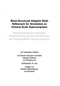
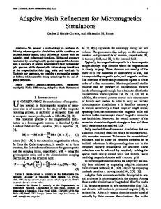
4.4.1 Numerical Configuration Application of the method of lines with a finite difference second order discretization in space implies a discretization of the Laplacian operator in (4.24) and thus, leads to a system of nonlinear ODEs. Finally, the time integration is then performed using a Strang operator splitting scheme that considers on the one hand, a high order method like Radau5 [18], based on implicit Runge-Kutta schemes for stiff ODEs, that solves the reaction term using adaptive time integration tools and highly optimized linear systems solvers. And on the other hand, another high order method like ROCK4 [1], based on explicit stabilized Runge-Kutta schemes, that solves the diffusion problem. In the case of D = 1 and k = 1, the velocity of the self-similar traveling wave is √ √ v = 1/ 2 and the maximal gradient value reaches 1/ 32. The structure of the wave can be observed in Figure 4.10 with an uniform discretization of 5001 points of the interval [−70, 70] and a time varying in [0, 30] divided into eight time intervals.
Fig. 4.10: Standard KPP traveling wave, discretization with 5001 points on the [−70, 70] region. Self-similar solutions for eight time intervals after the initial condition
The key point of this illustration is that the velocity of the traveling wave is proportional to (k D)1/2 , whereas the maximal gradient is proportional to (k/D)1/2 . Thus, switching to values k = 10.0 and D = 0.1, the velocity is preserved, but the maximal gradient is multiplied by a factor of 10 and introduces stiffness in the equation, as presented in Figure 4.11. For the spatial discretizations considered, the wave, however “stiff”, is always well solved on the considered grid. 4.4.2 Implementing Adaptive Grid As we have seen in the previous figures, we are mainly concerned with the simulation of propagating reaction fronts, spatially very localized. Hence, as soon as we consider higher spatial gradients, the precision of the numerical approximations will be guaranteed only
56
4. TEST-CASES
Fig. 4.11: “Stiff” KPP traveling wave, discretization with 5001 points on the [−70, 70] region. Self-similar solutions for eight time intervals after the initial condition
if very fine spatial discretizations are taken into consideration. In this context, uniform grids not only need important memory requirements in order to stock data, but also imply a very inefficient time consumption strategy, considering that important chemical activity takes place only on a very low percentage of the spatial domain, in the neighborhood of the wavefront. Therefore, in this study, we will consider the resolution of propagating wavefronts using a grid adaptation technique based on a multiresolution (MR) technique. In particular, we consider the reaction-diffusion system, KPP. The code that solves this problem using MR is given and supplies the executable calcul mr.x, after compilation. In order to run the program, we just need to type ./calcul mr.x into a terminal window, but first, we need to define the computing parameters included in the file input mr. This file must be placed in the same directory where we have put the executable. input mr gathers all the parameters that we are able to modify in order to conduct a complete case study. They are detailed in what follows. input mr • -70., 70., 1 :left and right limits of the domain, number of roots The spatial domain [−70, 70] is taken as an example, as we have previously seen the corresponding results. Usually, the only restriction is that the wavefront should be far enough from the boundaries in order to remain coherent with the homogeneous Neumann boundary conditions. The roots are equally distributed into the spatial domain while the phenomenon is spatially very localized, does a high number of roots have any negative/positive impact for this kind of application?
4.4. Nonlinear reaction-diffusion equation: the KPP equation
57
• 512 :time iterations Number of time integration steps. If the initial condition is already the traveling wave, a self-similar profile should be numerically reproduced for any time, what happens for another initial condition? • 20 :finest grid level Finest spatial discretization considered which gives the maximal level of spatial resolution. From a practical point of view, this parameter avoids memory overflow and fixes the finest grid that can be considered, but should it obey any physical feature? The actual maximal level obtained, does it (only) depend on the problem or does it (only/also) change according to other computing parameters? • 3 :minimum grid level Coarsest spatial discretization considered. From a practical point of view, it avoids searching space scales not present in the problem, however, should its choice depend on other parameters? • 1 :interpolation polynomial stencil Considering a centered polynomial interpolation, this parameter defines the order of interpolation from the number of cells considered into the stencil, 2s + 1 (in this example, the center cell plus 1 at each side, s = 1). Higher orders should yield higher/lower compression rates (less/more cells on the adapted grid)? The compression is defined as the ratio between the number of leaves and the cells on the finest grid. • 0.1 :threshold value ==> epsilon Thresholding value at the possible finest grid level (20 in this example), usually denoted as ε. Which are the thresholding values at the other grid levels? For a fixed ε, is it possible not having any cells on the finest grid and what could it mean in terms of MR error bound? • 0. :initial time output Initial time to save results. It should be greater or equal to zero (0) which is the initial time domain. • 6. :time step output Results will be saved with this time frequency starting from the initial time output (0 in this example). • 30. :final time Final time domain. Notice that the integration time step is 30/512 in this case.
58
4. TEST-CASES
• 1.d-1 :diffusion coefficient KPP diffusion coefficient D. In this case we consider kD = 1 in order to keep the same speed for all the possible configurations. How does the higher spatial gradient change? Which is the impact in terms of grid adaptation? And in terms of time consumption? For all the other parameters fixed, can we deduct from the results any changes in the spatial scales of the problem? Which are the equivalent uniform grids needed? • 0 :initial condition 0:continuous; 1:discontinuous We either start the time integration from the analytical solution (case 0) or from a discontinuous condition (case 1). Do we find different behaviors in terms of spatial scales? The initial condition is centered at ≈ 30% of the space domain, starting from the left boundary. The files generated are called: Champs t(time ∗ 100) niv(max level) s(s) eps(ε).dat and for each leaf, the following values are stocked in a column-fashioned way:
x
grid level
∆x
β
BIBLIOGRAPHY
[1] Abdulle, A. [2002]. Fourth order Chebyshev methods with recurrence relation, SIAM J. Sci. Comput. 23(6): 2041–2054 (electronic). [2] Adams, N. A. and Shariff, K. [1996]. A high-resolution hybrid compact-eno scheme for shock-turbulence interaction problems, J. Comp. Phys. 127: 27–51. [3] Ar`andiga, F., Donat, R. and Harten, A. [1999]. Multiresolution based on weighted averages of the hat function II: Non-linear reconstruction techniques, SIAM J. Sci. Comput. 20(3): 1053–1093. [4] Bell, J., Berger, M. J., Saltzman, J. and Welcome, M. [1994]. Three-dimensional adaptive mesh refinement for hyperbolic conservation laws, SIAM J. Sci. Comput. 15: 127–138. [5] Berger, M. J. and Colella, P. [1989]. Local adaptive mesh refinement for shock hydrodynamics, J. Comput. Phys. 82: 67–84. [6] Berger, M. J. and Oliger, J. [1984]. Adaptive mesh refinement for hyperbolic partial differential equations, J. Comput. Phys. 53: 484–512. [7] Bihari, B. L. and Harten, A. [1997]. Multiresolution schemes for the numerical solution of 2-D conservation laws I, SIAM J. Sci. Comput. 18(2): 315–354. [8] Bramkamp, F., Gottschlich-M¨ uller, B., Hesse, M., Lamby, P., M¨ uller, S., Ballmann, J., Brakhage, K. H. and Dahmen, W. [2003]. H-adaptive multiscale schemes for compressible Navier-Stokes equations - polyhedral discretization, data compression and mesh generation, in J. Ballmann (ed.), Flow modulation and fluid-structureinteraction at airplane wings, Vol. 84 of Numerical notes on Fluid Mechanics, Springer, pp. 125–204. [9] Bramkamp, F., Lamby, P. and M¨ uller, S. [2004]. An adaptive multiscale finite volume solver for unsteady and steady flow computations, J. Comp. Phys. 197(2): 460–490. [10] Brandt, A. [1977]. Multi-level adaptive solutions to boundary value problems, Math. Comp. 31: 333–390.
60
BIBLIOGRAPHY
[11] Cohen, A. [2000]. Wavelet methods in numerical analysis, Vol. 7 of Handbook of Numerical Analysis, P.G. Ciarlet and J.L. Lions, editors, Elsevier, Amsterdam. [12] Cohen, A., Daubechies, I. and Feauveau, J. C. [1992]. Biorthogonal bases of compactly supported wavelets, Comm. Pure Appl. Math. 45: 485–560. [13] Cohen, A., Dyn, N., Kaber, S. M. and Postel, M. [2000]. Multiresolution finite volume schemes on triangles, J. Comput. Phys. 161: 264–286. [14] Cohen, A., Kaber, S. M., M¨ uller, S. and Postel, M. [2003]. Fully adaptive multiresolution finite volume schemes for conservation laws, Math. Comp. 72: 183–225. [15] Daru, V. and Tenaud, C. [2004]. High order one-step monotonicity preserving schemes for unsteady flow calculations, Journal of Computational Physics 193: 563– 594. [16] Daru, V. and Tenaud, C. [2009]. Numerical simulation of the viscous shock tube problem by using a high resolution monotonicity-preserving scheme, Computers & Fluids 38: 664–676. [17] Gottschlich-M¨ uller, B. and M¨ uller, S. [1999]. Adaptive finite volume schemes for conservation laws based on local multiresolution techniques, in M. Fey and R. Jeltsch (eds), Hyperbolic problems: Theory, numerics, applications, Birkh¨auser, pp. 385–394. [18] Hairer, E. and Wanner, G. [1996]. Solving ordinary differential equations II, second edn, Springer-Verlag, Berlin. Stiff and differential-algebraic problems. [19] Harten, A. [1994]. Adaptive multiresolution schemes for shock computations, Journal of Computational Physics 115: 319–338. [20] Harten, A. [1995]. Multiresolution algorithms for the numerical solutions of hyperbolic conservation laws., Communications on Pure and Applied Mathematics 48: 1305–1342. [21] Hill, D. J. and Pullin, D. I. [2004]. Hybrid tuned center-difference-weno method for large eddy simulations in the presence of strong shocks, J. Comp. Phys. 194: 435–450. [22] Jiang, G.-S. and Shu, C.-W. [1996]. Efficient implementation of weighted eno schemes, Journal of Computational Physics 126: 202–228. [23] Lax, D. and Wendroff, B. [1960]. Systems of conservation laws, Communications on Pure and Applied Mathematics 13: 217–237. [24] LeVeque, R. J. [1992]. Birkh¨auser.
Numerical Methods for Conservation Laws, 2nd edn,
BIBLIOGRAPHY
61
[25] Moin, P. and Mahesh, K. [1998]. Direct numerical simulation: A tool in turbulence research, Annual Review of Fluid Mechanics 30: 539–578. [26] M¨ uller, S. [2003]. Adaptive multiscale schemes for conservation laws, Vol. 27 of Lecture Notes in Computational Science and Engineering, Springer-Verlag, Heidelberg. [27] Postel, M. [2001]. Approximations multi´echelles, Ecole de printemps de m´ecanique des fluides num´erique, Aussois. [28] Qiu, J. and Shu, C. W. [2004]. Hermit weno schems and their application as limiters for runge-kutta discontinuous galerkin method: one-dimensional case, J. Comp. Phys. 193(1): 115–135. [29] Ren, Y. X., Liu, M. and Zhang, H. [2003]. A characteristic-wise hybrid compact-weno scheme for solving hyperbolic conservation laws, J. Comp. Phys. 192(2): 365–386. [30] Roussel, O., Schneider, K., Tsigulin, A. and Bockhorn, H. [2003]. A conservative fully adaptive multiresolution algorithm for parabolic PDEs, J. Comput. Phys. 188(2): 493–523. [31] Shu, C. W. [1997]. Essentially non-oscillatory and weighted essentially non-oscillatory schemes for hyperbolic conservations laws, NASA/CR-97-206253 and ICASE Report 97-65 . [32] Shu, C. W. and Osher, S. [1988]. Efficient implementation of essentially nonoscillatory shock-capturing schemes, Journal of Computational Physics 77: 439–471. [33] Shu, C. W. and Osher, S. [1989]. Efficient implementation of essentially nonoscillatory shock-capturing schemes, II, Journal of Computational Physics 83: 32–78. [34] Strang, G. [1968]. On the construction and comparison of difference schemes, SIAM J. Numer. Anal. 5: 506–517. [35] Suresh, A. and Huynh, H. T. [1997]. Accurate monotonicity-preserving schemes with runge-kutta time stepping, Journal of Computational Physics 136: 83–99. [36] Titarev, V. A. and Toro, E. F. [2002]. Ader: Arbitrary high order godunov approach, Journal of Scientific Computing 17(1–4): 609–618. [37] Voss, A. and M¨ uller, S. [1999]. A manual for the template class library igpm t lib., Technical Report 197.