Nathan A. Carr and John C. Hart / Fast Reclustering each on a 100K face model, needing 20s to converge after 78 iterations. Our improvements capitalize on ...
Eurographics Symposium on Geometry Processing (2004) R. Scopigno, D. Zorin, (Editors)
Two Algorithms for Fast Reclustering of Dynamic Meshed Surfaces Nathan A. Carr and John C. Hart University of Illinois Urbana-Champaign
Abstract Numerous mesh algorithms such as parametrization, radiosity, and collision detection require the decomposition of meshes into a series of clusters. In this paper we present two novel approaches for maintaining mesh clusterings on dynamically deforming meshes. The first approach maintains a complete face cluster tree hierarchy using a randomized data structure. The second algorithm maintains a mesh decomposition for a fixed set of clusters. With both algorithms we are able to maintain clusterings on dynamically deforming surfaces of over 100K faces in fractions of a second. Categories and Subject Descriptors (according to ACM CCS): I.3.3 [Computer Graphics]: Geometric algorithms
1. Introduction The clustering of a mesh into collections of homogeneous collections of triangles is a well studied problem in computer graphics with applications in texture mapping, collision detection, radiosity and compression [SWG∗ 03, LPRM02, GWH01, GLM96, HSA91, KG00]. The maintenance of these clusters during the deformation of a mesh is much less studied, but can be important when dynamically updating cluster-based graphics solutions during modeling or animation. This paper explores two algorithms for maintaining good clusters on moving meshes of over 100K faces in a fraction of a second on a modern personal computer. The first algorithm constructs and maintains a hierarchical cluster that equivocates reclustering with maintaining a balanced tree of e.g. surface area, triangle count, sample distribution, or spatial spread. The challenge then becomes one of ensuring the clusters remain connected and round. We describe a novel application of Bloom filters, a data structure designed to provide fast probabilistic answers to set queries, to maintaining and reducing the perimeter lengths of the clusters. The Bloom filter data structure can get quite large for large meshes, but a careful analysis of its parameters coupled with run-length encoding of the data structure leads to an amenable implementation on current personal computers, e.g. we can recluster a 70K face bunny in 800ms using 22MB of Bloom-filter memory (156MB uncompressed). c The Eurographics Association 2004.
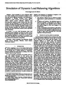
Figure 1: Simplified Buddha model (100K faces) being interactively deformed and automatically re-clustered (with 256 clusters) at 10Hz. Clusters are optimized for planarity and compactness.
The second algorithm improves iterative clustering, which grows clusters from a set of cluster centers, then finds better cluster centers for the resulting clusters, and repeats, e.g. [SWG∗ 03]. These iterations are costly, running about 250ms
Nathan A. Carr and John C. Hart / Fast Reclustering
each on a 100K face model, needing 20s to converge after 78 iterations. Our improvements capitalize on cluster coherence to accelerate these iterations. The first maintains a separate heap for each cluster to accelerate the region growing and erosion algorithms used to recompute cluster centers, resulting in a 2.5× speedup. The second improvement is based on the observation that some clusters converge before others, and keeping track of which clusters have changed reduces the per-iteration costs after 30 iterations to 10% of the version accelerated by the first improvement. These two improvements allow us to execute 78 reclustering iterations of a 100K-face mesh in less than a second. These two algorithms accelerate the clustering of dynamic meshes to support interactive updates. The hierarchical algorithm is especially well suited for hierarchical radiosity of dynamic scenes and collision detection between articulated objects. Both algorithms can be guided toward yielding the compact planar clusters that are useful for the reparameterization and signal-sensitive texture mapping needed to adaptively sample a deforming surface properly. Moreover, the improvements can be used to simply reduce the lengthy cluster preprocessing of large static meshes. 2. Previous Work Many algorithms exist in the literature for partitioning graphs. Since any dual representation of a mesh provides a graph, these algorithms may directly be applied. Shi and Malek introduced the concept of finding normalized cuts on a graph, and applied their result to image segmentation for use in computer vision [SM00]. Such approach was attempted by Katz and Taln for the decomposition of meshes but found mixed results[KT03]. Furthermore, the approach taken by Shi and Malek for solving the NPhard problem is involves solving the eigenvalue problem for rather large systems, so does not provide a constructive approach for adaptive graphs. Karypis and Kumar developed an algorithm that performs k-way partitioning of a graph into k disjoint connected subgraphs [KK98]. They attempted to form sub-graphs that are balanced, and whose resulting cut is minimal. The balance constraint forms sub-graphs whose sum of scalar vertex weights are all nearly equal. The minimal cut tries to reduce the sum of the edge weights crossing between partitioned sub-graphs. Although the results provided by this algorithm are reasonably fast and of good quality, the solution must be recomputed from scratch for any small perturbation in the graph. Garland et al. [GWH01] presented an agglomerative method for constructing a complete face cluster hierarchy for manifold meshes. Iterative edge contraction is performed on the dual graph of the mesh to construct the face hierarchy. Although reasonably fast, running in O(vlgv) for v vertices in the dual graph, the issues of maintaining such a hierarchy
on dynamically deforming meshes are not addressed by this research. Greedy region growing methods are another popular means for breaking a mesh into a collection of charts. They have the benefit over hierarchical clustering methods in that they optimize for a fixed set of face clusters, rather than all levels of a complete hierarchy. The greedy regions growing algorithms may be recursively applied to sub-clusters to build a full tree in a top down manner. Partition choices made higher in the tree may lead to poor clustering lower in the tree. They are often more expensive than bottom-up agglomerative approaches, making them less suitable for applications such as hierarchical radiosity that rely on a complete hierarchy. Levy et al. [LPRM02], Cohen-Steiner et al. [CSAD04], Schlafman et al. [STK02], and Sander et al. [SWG∗ 03] proposed greedy region growing algorithms for forming clusters. Seed faces are selected on the mesh, and greedy regions growing is performed in parallel outward from the seed faces to form the resulting clusters. The algorithms differ by their selection of seed faces as well as chosen metrics for guiding patch growth. Levy et al. chooses seeds only once by performing feature detection on the mesh. The algorithms provided by Schlafman et al. , Cohen-Steiner et al. , and Sander et al. are nearly identical, relying on a k-means style optimization strategy based off of Lloyd’s algorithm [Llo82]. New seed faces are computed using the cluster information from the greedy region growing process, leading to an iterative scheme that is repeated until the face seeds do not change and convergence is reached. Although the rate of convergence for clustering using kmeans style optimization is reasonably fast, the method may still take on the order of minutes to compute for reasonably sized meshes. Even when close to the solution the cost of a single k-means iteration for a large mesh may be high, preventing the algorithm from being useful in adaptive mesh environments. Katz and Taln present a method for forming a hierarchical decomposition of a mesh into sets of meaningful components [KT03]. Their underlying algorithm is similar to that proposed by Schlafman et al. and Sander et al. , however, they further improve segmentation quality by resolving boundaries between clusters with a min-cut algorithm. The metrics guiding the method do not optimize for developability or compactness, so it is not ideally suited for mesh parametrization. Further, the algorithm relies on computing all-pairs shortest paths on the dual graph of the mesh which is too costly for real-time application. 3. Dynamic Hierarchical Clustering Some clustering methods are hierarchical, collecting clusters into larger amalgams to provide multiresolution access to the faces of a mesh, such as for hierarchical radiosity [GWH01]. c The Eurographics Association 2004.
Nathan A. Carr and John C. Hart / Fast Reclustering
These offline techniques generate a tree of well-shaped clusters balanced according to a target metric. This section describes a fast rebalancing algorithm for rearranging the cluster hierarchy under a dynamic metric. We use Bloom filters in Section 3.1 as a fast method for estimating cluster perimeter length, and incorporate this goal as a second metric such that the rebalancing method described in Sec. 3.2 maintains round and contractible clusters. We start by defining the imbalance of a node n in a hierarchical face clustering as if n is a leaf, 0 δl /δr − 1 if δl > δr , (1) βn = δr /δl − 1 otherwise. where as before δl and δr are the importance distribution metric of the left and right children of n respectively. The imbalance indicates how much heavier one child is as a percentage of the weight of the other. When the imbalance of a node reaches some acceptability threshold, the hierarchy needs to be rebalanced. We rebalance the hierarchy with a greedy search over local perturbations of the tree described later in Section 3.2. However, tree perturbation can result in bad clustering, where sibling clusters sharing few edges are merged into long skinny parent clusters. Section 3.1 describes a fast method for estimating the number of shared edges between two clusters, and this estimate can help determine which tree perturbations to avoid. 3.1. Cluster Perimeter Estimation Given two nodes in the tree ni and n j , we desire to know the total length of the shared border between their corresponding clusters. This length can be found as the length of the intersection of the set of perimeter edges of cluster ni with the set of perimeter edges of cluster n j . But maintaining complete perimeter edge sets at every node in the tree is prohibitively expensive. To reduce memory and especially computation requirements, we instead use a randomized data structures that approximates these perimeters and measures shared boundary length more efficiently. Bloom Filters. Bloom filters are space and time efficient data structures for answering fast set queries with controlled error [Blo70]. A Bloom filter B(X) = (v, {hi }ki=1 ) operates on a subset X of some domain space X, and is comprised of a bit-vector v of m bits, and a set {hi }ki=1 of k hash functions hi : X → {1, 2, . . . , m}. To insert an element x ∈ X into B(X) we set the bits in v indexed by hi (x) for all i ∈ 1 . . . k. An element x is predicted by B(X) to be in X if the bits in v indexed by the k hash functions on x are all set. This approach prevents false negatives; if the bit in v indexed by any hi (x) is not set, then x 6∈ X. But there may be false positives; there may exist y ∈ X \ X such that every bit in v indexed by an hi (y) is set. The error rate (probability of a false positive) can c The Eurographics Association 2004.
be controlled by increasing the number hash functions k and the bit-vector length m. We Bloom filter the perimeter edge sets of every cluster in the hierarchy. First a unique id is assigned to every edge in the mesh. Then we construct a perimeter bit vector v of a cluster by hashing the ids of the edges in its perimeter. The Manhattan metric (L1 norm) on this bit vector, denoted ||vn ||, is the edge length of this perimeter predicted by the Bloom filter. The shared boundary between two clusters corresponding to two nodes i and j is predicted as the number of set bits the two vectors vi and v j have in common, or more concisely ||vi &v j ||. We store a perimeter bit vector vn at every node n in the binary tree. The perimeter bit vector of a leaf node is constructed by hashing the ids of the edges in its cluster’s perimeter. The perimeter bit vector of a parent is computed by the element wise exclusive-or of the bit vectors of its two children, which resets the bits corresponding to the shared edges of its children’s perimeters. The hashing functions, on which Bloom filters depend, can and do collide, introducing false positive errors. Section 3.3 shows this error is strictly a function of the height of the tree and the number of bits hashed at the leaves. Hence local tree perturbations do not accumulate additional error in the approximation. Perimeter Metric. We define a perimeter metric γn for every tree node n as � 0 if n is a leaf, γn = ||vl || + ||vr || + α| ||vl || − ||vr || | otherwise, (2) where vl and vr are the perimeter edge set bit vectors for the left and right child of node n respectively. The node’s perimeter metric is a function of the children’s perimeters (instead of its own perimeter) because the tree perturbation methods described next alter the child perimeters, but leave the node’s perimeter unchanged. The value α is a freely chosen parameter that gives some preference to balanced perimeter lengths. If α = 0, then the metric may be small even though one sibling’s perimeter is nicely rounded while the other’s is long and thin. We have found setting α = 1/4 suffices. 3.2. Cluster Tree Rebalancing Finding a good hierarchical face clustering becomes the task of finding a binary tree with every node n suitably balanced (according to the imbalance βn ) and corresponding to a well-shaped cluster (according to the perimeter metric γn ). We search the space of all such hierarchies with a greedy minimization that explores perturbations of the children and grandchildren of each node. We explore two kinds of perturbations: rotations and grandchild swapping. Figure 2 demonstrates half of the tree rotations available
Nathan A. Carr and John C. Hart / Fast Reclustering
C A B (a)
A
B B C (b)
A C (c)
A B C D A C B D A DB C (d) (e) (f ) B tree C D Figure 2:AThe (a) can be rotated into both configurations (b) and (c) because the order of children within a node is irrelevant. The grandchildren (d) can likewise be swapped into configurations (e) and (f).
to a node. The relevant children and grandchildren of a node are shown in (a). A standard rotation leads to configuration (b). However, since the order of the children within a node is irrelevant, switching grandchild A with B before the rotation leads to (c). We also investigate the two opposite rotations where the right � child is promoted. Figure 2 also demonstrates the 42 = 6 possible pairings of four grandchildren into two child nodes, organized into three different configurations (d),(e) and (f). To maintain triangle cluster coherence, every tree node must correspond to a simply-connected cluster of triangles. Both the rotation and grandchild swap may violate this property. We prune the available perturbations to better maintain connected partitions. Of the four rotations, we select only the one whose new grandchild pairing has the largest estimated shared edge length. Of the grandchild swaps, we reject the ones that do not meet or exceed the estimated shared edge lengths between the existing grandchild pairings. The perimeter metric and imbalance are then evaluated on the remaining perturbations. To further minimize perimeter length, we fix an imbalance threshold τ. If a node’s imbalance exceeds τ, we choose the perturbation with the smallest perimeter metric that brings the node closer to balance. If the node’s imbalance is already within τ, we choose the perturbation with the smallest perimeter metric whose imbalance remains below τ. If a rotation or grandchild swap is found and implemented, newly grouped descendants might, though rarely, violate the imbalance threshold τ. After a rotation we rebalance the parent of the newly paired grandchildren. After a grandchild swap, we rebalance both children of the base node. Construction. Construction of the initial face cluster hierarchy is performed bottom-up. The lossy nature of the Bloom filtering of perimeter length prevents triangle insertion into the tree in a top down manner. A single triangle is selected
from the mesh to form the first node of the tree. Triangles are added to the hierarchy from a breadth first traversal expanding from this initial triangle. Each triangle is inserted at the bottom of the tree by forming a new two-triangle cluster with an adjacent triangle that has already been inserted in the tree. The insertion of each new triangle into the tree requires rebalancing to minimize the prescribed metrics. For each new triangle, we rebalance all of the nodes in its ancestry, from the new two-triangle cluster all the way to the tree’s root. Hence, for reasonable meshes, a balanced hierarchy is constructed in approximately O(n log n) time, where n is the number of triangles. Algorithm Rebalance(Node n) Evaluate metrics β(n) and γ(n) Initialize the best choice n∗ = n If (β(n) > τ) Then For n0 ∈ Perturbations(n) If (γ(n0 ) < γ(n∗) and β(n0 ) < β(n)) n∗ = n0 Else For n0 ∈ Perturbations(n) If (γ(n0 ) < γ(n∗) and β(n0 ) < τ) n∗ = n0 Replace n with n∗ If n∗ was a rotation right Then Rebalance(RChild(n)) Else If n∗ was a rotation left Then Rebalance(LChild(n)) Else If n∗ was a granchild swap Rebalance(LChild(n)) Rebalance(RChild(n)) If (p = Parent(n)) Rebalance(p) Figure 3: Algorithm to rebalance the tree after the metric of a single node has changed. Maintenance. When the signal or shape of a set of triangles changes, the meshed atlas needs to be rebalanced. This rebalancing occurs by calling Rebalance(n) on each leaf node n whose cluster contains at least one of the changed triangles. Note that this results in a walk up the ancestry of each of these leaf nodes, even though they may share common ancestors. Simultaneously updating the metrics of all of the leaf nodes sends the tree too far out of balance to be easily recovered by the greedy local perturbation search. Assuming a constant number of changed leaf nodes, maintenance is thus, on average, an O(log n) time process. 3.3. Analysis This section derives the error rate of the Bloom filter as a function of its level in the hierarchy, which leads to a heuristic for choosing an appropriate bit-vector size m. An additional outcome of this analysis is the discovery that hashing two bits per edge instead of one provided better cluster shapes. We first consider the error imposed by hashing. Suppose a node corresponds to a cluster with a perimeter of e edges. c The Eurographics Association 2004.
Nathan A. Carr and John C. Hart / Fast Reclustering
The node contains a bit vector v of m elements that underestimates the perimeter edge length, because collisions may occur in the hashing of perimeter edges. If we assume a uniform hashing distribution, the probability that a particular bit of v will be zero is ((m − 1)/m)e . The expected perimeter length is the expected number of bits set in v, � � �e � m−1 E[||v||] = m 1 − (3) m It follows that the expected number of collisions that occur when constructing v from the e perimeter edges is the difference between the actual perimeter edge length e and the expected perimeter length underestimate E[coll] = e − E[||v||].
(4)
We now define Ploss to be percentage of bits (perimeter edges) lost due to collisions Ploss =
between the clusters of C1 and C2 . In other words E1 and E2 are not mutually independent, therefore Pr[E1 E2 ] 6= Pr[E1 ]Pr[E2 ]. Thus, we predict the percentage of a cluster’s edges that are shared with a single neighboring cluster. If clusters form equilateral triangles, then neighboring clusters each share 1/3 of their edges. Quadrilateral clusters share 1/4 of their edges, and hexagonal clusters share 1/6. We measured the mean fraction of shared edges resulting from our clustering method on several meshes, and found it surprisingly to uniformly approximate 1/5. We now examine the growth rates of cluster perimeters under various neighboring predictions. Let c denote the assumed percentage of edges a cluster shares with a single neighboring cluster, e.g. 1/3, 1/4 or 1/6. Let ei be the perimeter edge length of a cluster at level i, where i = 0 corresponds to a leaf node. Thus e0 = 3 and ei = 2ei−1 − 2cei−1 ,
E[coll] e
(5)
This allows us to compute Table 1, which shows the chances that an edge is lost due to a hashing collision at the single-triangle leaf nodes, by computing Ploss for hash functions that set one bit per edge e = 3 and various bitvector lengths m. For later reference, we also compute the leaf-node Ploss for hash functions that set two bits per edge by setting e = 6. bit vector size m
Ploss , e = 3
Ploss , e = 6
2 KBytes 4 KBytes 8 KBytes
0.0488% 0.0244% 0.0122%
0.122% 0.061% 0.031%
= 2(1 − c)ei−1 , = 3(2(1 − c))i .
(6)
Table 2 illustrates the perimeter growth rate under various edges-shared percentages c. triangles
edges
c = 1/3
c = 1/4
c = 1/6
1K 8K 256K 1M
1,623 12,580 395,433 1,577,852
53 126 532 946
173 584 4,437 9,976
496 2,296 29,539 82,053
Table 2: Cluster perimeter edge lengths ei as a function of cluster size and shared edge percentage c.
Table 1: Bit loss rate at leaf nodes. We now develop a model to extend Ploss to reveal the percentage of bits lost at every level higher in the tree. Suppose a parent node P has two children C1 and C2 each having n bits set. Let E1 = Event that a particular bit in v(C1 ) is 1, E2 = Event that another particular bit in v(C2 ) is 1, E3 = Event that yet another particular bit in v(P) is 1. Note that the probabilities of the first two events Pr[E1 ] = Pr[E2 ] = n/m. Since the bit vector in P is the exclusive-or of the bit vectors of its two children, we can express the probability that a given bit is set in v(P) as Pr[E3 ] = Pr[E1 ∪ E2 ] − Pr[E1 E2 ] = Pr[E1 ] + Pr[E2 ] − 2Pr[E1 E2 ] = 2n/m − 2Pr[E1 E2 ] We do not know a priori the number of edges shared c The Eurographics Association 2004.
As expected, the growth of the perimeter edge set grows much slower than the number of triangles in the cluster, which suggests the efficiency of Bloom filters when working with large meshes. It is interesting to note that decreasing c from triangular (c = 1/3) to hexagonal (c = 1/6) does not imply rounder clusters. In fact the perimeter lengths increase which implies skinnier clusters that reach more neighboring clusters. An expression can now be formulated for Pr[E1 E2 ] using our cluster connectedness assumption c. We define the two events E2b = a particular shared border bit in C2 is 1, E2p = a particular non-shared perimeter bit in C2 is 1. The probability of Pr[E1 E2 ] may now be expressed Pr[E1 E2 ] = Pr[E1 ]Pr[E2 |E1 ], = Pr[E1 ](Pr[E2b |E1 ] + Pr[E2p |E1 ]), n� n� c + (1 − c) , = m m
Nathan A. Carr and John C. Hart / Fast Reclustering
and
tree size Pr[E3 ] = 2n(1 − c)(1 − n/m).
Using this model, the expected number of bits set in node P will be E[||w(P)||] = m × Pr [E3 ] 3 = n (1 − n/m) 2 We now have an expression that predicts the number of bits set in a node given the number of bits set in its two children. The expected number of collisions that have occurred higher up in the tree is E[coll(P)] = e(P) − E[||w(P)||]
(7)
where e(P) is the actual number of edges in the perimeter of the cluster corresponding to P. As before, Ploss (P) = E[coll(P)]/e(P). Error increases in our model due to collisions. As our bit vector is required to hold more and more edges, it becomes saturated. The effect of saturation is that more collisions occur and thus information is lost during the exclusive-or operation. Table 3 uses the above formulated model to show the percent loss occurring at various subtree levels. tree size
Ploss
leaves (tris)
m=2K
m=4K
m=8K
m=16K
1K 8K 256K 1M
14.67% 38.41% 85.30% 93.24%
7.80% 23.01% 73.04% 86.83%
4.03% 12.73% 55.71% 75.53%
2.05% 6.71% 37.17% 58.89%
Table 3: Perimeter Loss Rates, c = 1/4, 1 bit per edge. A loss rate of 50% at a given level of the tree implies that half of the perimeter bits have been lost or more concretely that our estimate of the edge length of the perimeter of our root cluster is half of its actual edge length. Although this may seem sloppy, we only need enough bits to make good judgements on which local tree perturbations to perform. At higher levels in our tree, the loss rate increases, but so too does the number of bits that are set, allowing us to still make good choices about what tree operations should be performed. In practice we found the loss at higher levels in the tree to be satisfactory. We did find that random collisions occurring very low in the tree proved fatal, leading the algorithm to make poor tree operation choices. To prevent this we chose to hash two bits per edge. Although our overall perimeter loss rate increased, we found that our clusters became better shaped (rounder) due to the increased information lower in the tree. Table 4 shows the expected perimeter loss using 2 bits per edge.
Ploss
leaves (tris)
m=2K
m=4K
m=8K
m=16K
1K 8K 256K 1M
26.15% 57.06% 92.41% 96.59%
14.68% 38.41% 85.30% 93.24%
7.81% 23.02% 73.04% 86.83%
4.03% 12.73% 55.71% 75.53%
Table 4: Perimeter Loss Rates, c = 1/4, 2 bits per edge.
3.4. Results We tested the rebalancing algorithm by randomly perturbing every leaf node’s δ by a factor ε ∈ [0.5, 2.0]. Table 5 compares the mean imbalance in the tree using a surface area metric to the mean imbalance after the application of the perturbation. In both cases the average imbalance remains below our threshold tolerance τ = 1. Average βn
model model
area weighted
area weighted +noise
cow
0.44
0.47
head
0.33
0.42
bunny
0.31
0.61
Table 5: Imbalance metric results showing good tree balance even under large importance perturbations with τ = 1. Table 6 details the memory and performance results for our reparametrization method. All tests were run on a 700 MHz Athlon processor. Our scheme achieves interactive to real-time rates depending on the size of the input mesh. model
triangles
size
build
reparam
bunny
69,451K
156MB
60.22s
0.85-1.3s
head
7,232K
16MB
4.42s
0.09-0.14s
cow
5,804K
13MB
3.66s
0.07-0.1s
Table 6: Reparameterization performance using uncompressed 8M bits per tree node. The memory requirements of an 8M bit/node hierarchy are substantial. The bottom of our face cluster tree has only sparsely set bit vectors, but these nodes account for most of the tree. Compression of Bloom filters is an area of recent interest [Mit01]. A simple run-length encoding of the bit vectors reduced memory requirements by more than 85%, as shown in Table 7. c The Eurographics Association 2004.
Nathan A. Carr and John C. Hart / Fast Reclustering
model
triangles
size
build
rebalance
bunny
69,451K
22MB
183.69s
0.7-0.8s
head
7,232K
2.6MB
10.08s
0.08-0.1s
cow
5,804K
1.8MB
8.41s
0.06-0.08s
Table 7: Reparameterization performance using compressed 8M bit fields per tree node.
Our initial tree build times tripled when using compressed bit vectors, though we attribute much of this increase memory allocation overhead from bit vector resizing. Tree rebalancing ran 20-50% faster with compressed bit vectors, which we attribute to reduced memory bandwidth, and the efficiency of computing ||w|| on a compressed bit vector.
level 2
Figure 4 shows the results of the Bloom filter clustering process on the cow model, showing levels 2,4, and 6 of face cluster tree (where level 0 is the root). At each level, cluster perimeter is minimized, and the cluster surface areas are balanced. 4. Adaptive k-means Style Clustering on a Surface As discussed in Section 2, Levy et al. [LPRM02], Schlafmen et al. [STK02], Cohen-Steiner et al. [CSAD04], and Sander et al. [SWG∗ 03] proposed greedy regions growing methods for chart construction. We chose to adapt the methods taken by latter three references for the following two reasons. First, these methods allow the mesh to be decomposed into any number of clusters. Secondly, they are all based on an iterative k-means type approach allowing the solution to be updated rather than re-computed during mesh changes. The approach by Cohen-Steiner et al. , does not attempt to favor compactness, and as a result is more efficient, but less suited to applications such as surface parametrization. For this reason we focus primary on the essentially identical methods proposed by Sander et al. (and Schlafmen et al. ) in describing our technique. 4.1. Background The algorithm presented by Sander et al. in [SWG∗ 03], can be broken down into two separate phases that are iteratively applied until convergence is reached: an outward region growing phase, and an inward growing phase. The outward region growing phase, grows clusters outward from a set of seed faces also referred to as cluster centers. Faces in the mesh are assigned to the cluster represented by their closest cluster center where distance is defined to be the shortest path in the dual graph. The inward growing phase performs a shortest path search inward on each cluster to determine the face that is most central to the cluster. These faces become the cluster centers for the next iteration of the algorithm. The c The Eurographics Association 2004.
level 4
level 6 Figure 4: Cow model clustered using Bloom filters. Levels 2, 4, and 6 of the face cluster hierarchy.
two phases are applied until convergence is reached and the cluster centers do not change(or a cycle is reached). Both the outward region growing phase and inward growing phase use Dijkstra’s search algorithm, touching every face in the mesh. Dijkstra’s algorithm has the well known running time of O((V + E) lgV ), or O(V lgV + E) when implemented with a Fibonacci heap[CLR90]. The latter approach, however, has a high cost hidden in constant factors. The overall running time for the algorithm is given
Nathan A. Carr and John C. Hart / Fast Reclustering
by O(I(V + E) lgV ), where I is the number of iterations required for convergence. 4.1.1. Initialization For every dual vertex u, a scalar distance DIST(u), and its closest cluster CLUSTER(u) is maintained. The distance is defined to be the minimum distance (along the dual graph) from u to its closest cluster center vertex whose cluster is given by CLUSTER(u). Sander et al. proposed the following edge distance metric between adjacent faces F and F 0 in the dual graph DIST(F, F 0 ) = (λ − (Nc · NF 0 ))||PF − PF 0 ||2
(8)
where PF and PF 0 are the location of the faces centers, Nc is the average normal of the region, and NF 0 is the normal for face F 0 . Sander chose the parameter λ = 1.0 giving no distance penalty to faces co-planar with the global region normal. Schlafman et al. proposed a similar metric DIST(F, F 0 ) = (1 − λ)(1 − cos2 (α)) + (λ)||PF − PF 0 ||2 . (9) Here α is the dihedral angle between the faces, and λ ∈ [0, 1] is freely chosen between the first term (angular distance) and the second term which approximates geodesic distance. For the purpose of forming planar compact patches, we prefer the metric in (8) over that provide in (9) since the latter relies on edge lengths to be on a similar scale to that of the angular distance term. At the start of the process k seed faces (dual vertices) are selected to act as centers for the mesh clustering process. These may be selected randomly, or via any number of heuristic approaches. The k-means strategy converges to a local minima, so the starting choice of seed faces impacts not only the number of iterations required for convergence, but also the quality of the resulting clusters. For achieving our starting seed configuration we use recursive coordinate bisection[Sim91], which forms initial clusters based on Euclidean (rather than geodesic) distances. Faces are treated as a 3D point-set using their centroid locations. We compute the center of mass for the point set, and its 3x3 inertial tensor matrix. The center of mass and the eigenvector corresponding to the minimum eigenvalue of the matrix defines a plane that minimizes the sum of squared distances between all points in the set and the plane. The cutting plane partitions the points into two spatially coherent groups. We recursively apply the process to divide the points into smaller sets until the number of sets equals the number of starting seeds. For each set we find the most central face (in the Euclidean sense) and use it as a starting seed face. 4.1.2. Phase 1: Outward Region Growing The cluster center vertices are assigned a distance of zero (since they are are zero distance from a cluster center), and
assigned to a unique cluster. All other dual vertices are assigned an infinite distance since their shortest paths to a cluster center are currently unknown. Cluster center vertices are then placed into a priority queue. At each step of the region growing process, a dual vertex u is removed from the top of the priority queue, and assigned to its closest cluster, CLUSTER(u). Relaxation is performed on the neighbor set v ∈ Ad j[u] of u, where Ad j[u] is the set of neighboring vertices attached by an edge to u in the dual graph. This is done by computing a distance d for each adjacent face that has not been assigned to a cluster. This distance is computed as follows: d = DIST(u)+DIST(u, v). If d is less than the currently known distance for v: DIST(v), then u is relaxed by setting DIST(v) = d and CLUSTER(v) =CLUSTER(u), and updating the location of v in the priority queue accordingly. Pseudocode for phase 1 of Sander’s algorithm is given in Algorithm 5. Algorithm Phase1(faceHeap H) while H 6= Ø u ← EXTRACT-MIN(H) C ← CLUSTER(u) C←C∪u for each v ∈ Adj[u] d ← DIST(u,v) if DIST(u) + d < DIST(v) DIST(v) ← DIST(u) + d CLUSTER(v) ← CLUSTER(u) if v ∈ H DECREASE-KEY( H,v,DIST(v)) Figure 5: Outward region growing algorithm implemented using a single heap.
4.1.3. Phase 2: Inward Region Growing Following phase 1, every face has been assigned to a cluster. The quality of each cluster is dependant on both the number of seed faces, and the choice of seed face locations. Phase 2 computes a new seed face for each cluster. The new seed face for each cluster is chosen to be the face whose distance (along the dual graph) to the cluster border is maximal. These new seed faces are found by placing the faces along the borders of each cluster onto a heap, and assigning them a zero distance. Regions are grown inward using the same Dijkstra search algorithm detailed in phase 1. The last face reached within each cluster during this inward growing process becomes the new seed face for the cluster. Using the updated seed faces, phase 1 may be applied to compute the new clusters. The two phases are iterated until convergence or a cycle is detected. c The Eurographics Association 2004.
Nathan A. Carr and John C. Hart / Fast Reclustering
4.2. Multiple Heaps To improve the running time of the algorithm we start by decomposing the problem into a collection of heaps, one per cluster. The algorithm proceeds in a manner similar to that presented in Figure 5. Rather than adding faces to a global heap during the relaxation process, faces are added to the heap whose cluster center is currently closest. The order in which faces are processed is handled by selecting the cluster heap whose top element has the minimum distance. This search may be accelerated by placing all clusters into a global priority queue (heap) represented by HG in algorithm 6. Algorithm Phase1_Optimized(globalHeap HG ) while HG 6= Ø C ← EXTRACT-MIN(HG ) u ← EXTRACT-MIN(HC ) C←C∪u for each v ∈ Adj[u] d ← DIST(u,v) if DIST(u) + d < DIST(v) DIST(v) ← DIST(u) + d CLUSTER(v) ← CLUSTER(u) if v ∈ Hi , Hi 6= HC DELETE( Hi ,v) else if v ∈ HC DECREASE-KEY( HC ,v,DIST(v)) else INSERT( HC ,v,DIST(v)) if HC 6= Ø u ← TOP(HC ) INSERT( HG ,C,DIST(u)) Figure 6: Optimization for the outward region growing process. Nested heap structure used to reduce search times.
By decomposing the problem into a collection of heaps, the inward region growing process (phase 2) may be handled separately for each cluster. This is done by iterating over the clusters, and performing the Dijkstra shortest path search inward from the cluster’s border to find the face that is most distant from the edge. Assuming every cluster grows to contain the same number of triangles, the running time of phase 1 is reduced to O((V lg(k) + (V + E) lg(V /k)), and phase 2 is reduced to O((V + E) lg(V /k)).
4.3. Border Sets The optimization presented above reduces the cost of executing a single iteration of the k-means process. The cost of each successive iteration, however, remains constant. Ideally c The Eurographics Association 2004.
we wish the iteration cost to decrease as it converges towards the solution. The key observation is that interactions on successive iterations occur on the borders between cluster regions. We store with each cluster C the set BC of triangles on its border. A triangle t is in BC if it belongs to the cluster C, but shares at least one edge with another cluster. If a cluster’s border set has not changed following an iteration of phase 1, then clearly the seed face for that cluster does not change either. In this case, phase 2 (the inward growing process) need not be performed for that cluster. The known border is also used to improve the performance of phase 1. The idea is that the current clusters provides a good starting guess for an iteration of phase 1. Rather than initializing each cluster’s heap HC with the cluster’s single seed face, we insert the cluster’s border set BC into its heap. Successive iterations of phase 1 are therefore performed starting with each cluster already grown out to its border. The cost of phase 1 is reduced to the movement of a few triangles between clusters on the frontiers between cluster regions. In the event that a cluster’s border set changes following phase 1, a new seed face must be computed for that cluster. We apply a phase 2 operation to that cluster to find the new cluster center. For phase 1, however, every face must the distance to its closest cluster center. This requires the distances within a cluster to be recomputed by growing the patch outward from its new cluster center to its border. In some cases, however, this situation may be avoided. If the result of performing a phase 2 operation on the cluster finds the cluster seed face unchanged, then the distances to the center may not need to be computed. In the case of the DIST () metric provided by Sander et al. , distances are impacted by the global chart normal so this optimization cannot be used. The last improvement is to note that that if a cluster C and all of its adjacent clusters Cad j remain unchanged after an iteration of phase 1 and phase 2, then C cannot grow outward during the next iteration of phase 1. Therefore, we do not place cluster C on the global head HG , or initialize C’s cluster heap HC with its border set. 4.4. Results These enhancements play a significant role in the performance of the clustering process and can be used to achieve the exact same solution as that proposed in [SWG∗ 03] and [STK02]. As the algorithm converges, the number of changing clusters decreases along with the processing time. Figure 7 shows the running time used on the horse model. The clustering process was seeded with k = 256 randomly chosen seeds, and took 80 iterations to converge. By using a separate heaps per clusters we achieved a 2.5× speedup. Keeping track of the changing clusters further reduces the running
Nathan A. Carr and John C. Hart / Fast Reclustering
time which decreases as the algorithm converges, providing over a magnitude speed-up over the original method.
deformations impacting all clusters. Deformation 1 on the graph shows the time required to cluster the model from scratch. Note that under some extreme deformations with k = 128 the running time equalled that of initially clustering the model from scratch. By increasing the number of clusters, the algorithm is able to find a local minimum with fewer iterations resulting in faster running times.
Figure 7: Clustering performance on the horse model containing 96,966 faces, using k = 312 and randomly chosen seed faces. The reduction in processing time when near the solution makes this algorithm practical for dynamic meshes. For any given deformation, the running times for our method greatly varied depending on the magnitude of deformation (from the last computed clustering) and the number of clusters impacted by the deformation. We tested models of varying size up to 100K faces, and found our re-clustering to run in under 1.0 second even for reasonably large deformations impacting the entire model. Figure 1 shows screen shots from an interactive modeling session with a 100K face Buddha model. The re-clustering times during the shown deformation took between 0.08−0.1 seconds on a 2.1GHz Athlon processor. Figure 8 shows the 69,451 face bunny model interactively deformed and reclustered with k = 256. Note how the clusters resist crossing high curvature regions of the model, as governed by the metric given in equation 8.
Figure 8: Re-clustering of bunny model containing 69,451 faces, using k = 256 and randomly chosen seed faces at 20Hz. Note the clusters maintain compact shape and avoid crossing high curvature regions of the mesh. Figure 9 shows how the performance of the reclustering method is impacted by the number of clusters under extreme
Figure 9: Reclustering times for the Buddha model (100K faces) undergoing 45 large deformations, with k=[128, 256, 512, 1024]. Lloyd’s algorithm for k-means clustering is only known to converge to some local minimum. For any given choice of starting seeds the potential arises for the clustering algorithm to get trapped in some poor local minimum. Furthermore, if may be desirable to minimize the number of clusters or let the clustering processes determine the number of clusters needed to meet some threshold error criteria. Both of these goals may be met by applying merging and splitting of clusters during the k-means process. Merging is be performed when two connected clusters are detected that may be combined to form a single cluster without introducing much error. Splitting is accomplished by adding an additional seed face to a cluster containing high error. Splitting may be used to introduce new clusters until the error falls below some threshold[SWG∗ 03]. A merge followed by a split (referred to as region teleportation), allows the algorithm to escape potentially poor local minima [CSAD04]. We have not yet implemented merging and splitting into our dynamic clustering system, but do not foresee any obstacles for this using our method. 5. Conclusions We have thus demonstrated two methods (one hierarchical, the other iterative) for reorganizing face clusters on a meshed surfaces. These methods run at interactive speeds (less than a second) for large models of 100K polygons and in realtime (less than 100ms) for smaller models of 10K polygons. c The Eurographics Association 2004.
Nathan A. Carr and John C. Hart / Fast Reclustering
It is interesting to note, in conclusion, that both algorithms rely heavily on sophisticated data structures to maintain the shared boundaries between clusters. The hierarchical reclustering method seems particularly well suited for collision detection of articulated deforming figures in games and virtual environments where face counts are held to a minimum. Examples of dynamic meshes in such applications could include the ability to dig holes and caves in terrain, or in general the manipulation of one’s environment to solve a problem. The main impediment preventing the widespread application of the hierarchical reclustering method is the size of Bloom filters. Simple RLE compression resulted in an 85% reduction in their storage. Other more sophisticated compression techniques could produce 100:1 and perhaps 1000:1 compression rates. Bloom filters produce a probabalistic result, so their compression need not even be lossless. Other compression methods in graphics have sacrificed quality for speed (e.g. the reduction of overdraw in compressed precomputed radiance transfer [SHHS03]). In the case of Bloom filters one could similarly sacrifice prediction quality for an additional boost in compression rate. The iterative reclustering method appears to be a good choice for interactive modeling systems, where one may want to maintain (and dynamically resample) a texture atlas during the modeling process. When clusters are formed on the basis of signal bandwidth, reclustering becomes a method for dynamically tuning a texture atlas to best reproduce the signal. For example, a painting system based on this concept allows the system to reproduce fine strokes [CH04], but was implemented using a multiresolution meshed atlas whose charts are not very “intuitively” organized. Reclustering into more round, flat charts as described here could lead to an atlas that, while perhaps not covering the texture domain as efficiently, would nevertheless contain fewer, larger charts that would be easier to navigate mentally by texture artists. References [Blo70]
[CH04]
[CLR90]
[GLM96]
G OTTSCHALK S., L IN M. C., M ANOCHA D.: OBBTree: A hierarchical structure for rapid interference detection. In Proc. SIGGRAPH 96 (1996), pp. 171–180. 1
[GWH01] G ARLAND M., W ILLMOTT A., H ECKBERT P. S.: Hierarchical face clustering on polygonal surfaces. In Proc. Interactive 3D Graphics (2001), ACM, pp. 49–58. 1, 2 [HSA91]
H ANRAHAN P., S ALZMAN D., AUPPERLE L.: A rapid hierarchical radiosity algorithm. In Proc. SIGGRAPH 91 (July 1991), pp. 197–206. 1
[KG00]
K ARNI Z., G OTSMAN C.: Spectral compression of mesh geometry. In Proc. SIGGRAPH 2000 (July 2000), pp. 279–286. 1
[KK98]
K ARYPIS G., K UMAR V.: Multilevel algorithms for multi-constraint graph partitioning. In Proc. Supercomputing 98 (Nov. 1998). 2
[KT03]
K ATZ S., TALN A.: Hierarchical mesh decomposition using fuzzy clustering and cuts. ACM Trans. on Graphics 22 (July 2003), 954–961. 2
[Llo82]
L LOYD S. P.: Least squares quantization in pcm. IEEE Trans. Inform. Theory 28 (1982), 129–137. 2
[LPRM02] L EVY B., P ETITJEAN S., R AY N., M AILLOT J.: Least squares conformal maps for automatic texture atlas generation. In Proc. SIGGRAPH 2002 (2002), ACM, pp. 362–371. 1, 2, 7 [Mit01]
M ITZENMACHER M.: Compressed Bloom filters. Proc. ACM Symp. on Principles of Distributed Computing (2001), 144–150. To appear: IEEE/ACM Trans. on Networking. 6
[SHHS03] S LOAN P.-P., H ALL J., H ART J., S NYDER J.: Clustered principal components for precomputed radiance transfer. Proc. SIGGRAPH 2003, ACM Trans. on Graphics 22, 3 (2003), 382–391. 11
B LOOM B.: Space/time tradeoffs in hash coding with allowable errors. Communications of the ACM 13, 2 (July 1970), 159–188. 3
[Sim91]
C ARR N. A., H ART J. C.: Painting detail. Proc. SIGGRAPH 2004, ACM Trans. on Graphics 23, 3 (Aug. 2004). 11
S IMON H. D.: Partitioning of unstructured problems for parallel processing. Computing Systems in Engineering 2 (1991), 135–148. 8
[SM00]
S HI J., M ALIK J.: Normalized cuts and image segmentation. IEEE Trans. on Pattern Analysis and Machine Intelligence 22, 8 (2000), 888– 906. 2
[STK02]
S HLAFMAN S., TAL A., K ATZ S.: Metamorphosis of polyhedral surfaces using decomposition. Computer Graphics Forum 21, 3 (Sept. 2002). 2, 7, 9
C ORMEN T., L EISERSON C., R IVEST R.: Introduction to Algorithms. McGraw-Hill, 1990. 7
[CSAD04] C OHEN -S TEINER D., A LLIEZ P., D ESBRUN M.: Variational shape approximation. Proc. SIGGRAPH 2004, ACM Trans. on Graphics 23, 3 (Aug. 2004). 2, 7, 10 c The Eurographics Association 2004.
[SWG∗ 03] S ANDER P. V., W OOD Z. J., G ORTLER S. J.,
Nathan A. Carr and John C. Hart / Fast Reclustering
S NYDER J., H OPPE H.: Multi-chart geometry images. In Proc. Sym. on Geom. Proc. (2003), pp. 146–155. 1, 2, 7, 9, 10
c The Eurographics Association 2004.