Aug 18, 2015 - Two-dimensional landslide dynamic simulation based on a velocity-weakening friction law. Abstract Surprisingly, hypermobility (high velocity ...
Original Paper Landslides DOI 10.1007/s10346-015-0632-z Received: 29 December 2014 Accepted: 18 August 2015 © Springer-Verlag Berlin Heidelberg 2015
Wei Liu I Siming He I Xinpo Li I Qiang Xu
Two-dimensional landslide dynamic simulation based on a velocity-weakening friction law
Abstract Surprisingly, hypermobility (high velocity and long runout) is a remarkable feature of large landslides and is still poorly understood. In this paper, a velocity-weakening friction law is incorporated into a depth-averaged landslide model for explaining the higher mobility mechanism of landslides. In order to improve the precision of the calculation, a coupled numerical method based on the finite volume method is proposed to solve the model equations. Finally, several numerical tests are performed to verify the stability of the algorithm and reliability of the model. The comparison between numerical results and experimental data indicates that the presented model can predict the movement of landslide accurately. Considering the effect of velocity-weakening friction law, the presented model can better reflect the hypermobility of landslide than the conventional Mohr–Coulomb friction model. This work shows that the application of a universal velocity-weakening friction law is effective in describing the hypermobility of landslide and predicting the extent of landslides. Keywords Velocity-weakening friction law . Depth-averaged landslide model . Hypermobility . Numerical simulation Introduction The gravity-driven granular mass flow of a landslide down a slope can be catastrophic to nearby populations and infrastructure (Davies and McSaveney 1999; Legros 2002; Davies et al. 2010; Sosio et al. 2012). However, the physical phenomena underlying natural landslides are still not entirely understood. One of the key challenges is to understand the origin of the apparent hypermobility of landslides during their propagation along a slope. In recent years, many transport mechanisms have been proposed to explain the hypermobility of landslides, including pore fluid pressure (Goren and Aharonov 2007, 2009; Iverson et al. 2010; Iverson 2012), air pockets (Fritz et al. 2003; Heller and Hager 2011), lubrication (De Blasio 2011; Massaro et al. 2011), fluidization (Okura et al. 2002; Ochiai et al. 2004; Xing et al. 2014), entrainment (Pitman et al. 2003; McDougall and Hungr 2005; Lê and Pitman 2009; Hutter and Luca 2012), and dynamic fragmentation (Gerolymos and Gazetas 2007; Cagnoli and Romano 2010). The model proposed by Iverson (1997) based on the Savage–Hutter model claimed that the effective stress is reduced by the rise in pore water pressure when the landslide slip surface passes through a saturated bed, and the frictional resistance is also reduced. Vardoulakis (2000) presented a basic mathematical structure of thermo-poro-mechanical model accounting for frictional heating and pore fluid pressure generation in the slip plane of a uniform slope. Goren and Aharonov (2007) investigated a thermo-poro-elastic mechanism that considered a temperature increase due to frictional heating, which causes thermal pressurization within a fluid-saturated shear zone—the pressure rise leading to a reduction in frictional resistance. All of these mechanisms highlight the importance of determining a low friction resistance of the sliding surface compared
with the actual friction resistance. Although these mechanisms are suitable for some site-specific landslides, no dominant mechanism stands out as an explanation for the hypermobility. Recently, an interesting phenomenon that the effective friction coefficient of landslides may change during movement, as evidenced by the laboratory experiments and extension observed in landslide deposits, has attracted many researchers (Gray et al. 1999; Rice 2006; Jop et al. 2006; Beeler et al. 2008; Dong et al. 2009, 2013; Lucas et al. 2014). A high-velocity rotary shear frictional testing apparatus was used to study the fast-moving and/or long-duration behavior of giant landslides, and the kinematics of these studied landslides were qualitatively depicted (Yano et al. 2009; Miyamoto et al. 2009; Ferri et al. 2010). Although laboratory experiments on granular flows have been able to reproduce the evolution of frictional coefficient on the sliding surface with the displacement and velocity of the moving mass, they fail in comparison to quantitative field observations to explain the hypermobility of gravitational flows that can travel great distances along small slopes (Davies and McSaveney 1999; Mangeney et al. 2007 ; Lucas and Mang eney 2007). Furthermore, Gray et al. (1999) considered that the bed friction angle is related to the avalanche positions, and a simple formula of bed friction angle was proposed to reproduce the experiment. Jop et al. (2006) proposed a rheological law for granular materials in which the friction coefficient depends on an inertial number. Rice (2006) and Beeler et al. (2008) suggested that flash heating between two rough, solid surfaces reduces the local shear strength of the contact area, leading to a decrease of the friction coefficient as a function of sliding velocity. Dong et al. (2013) proposed a velocity-displacementdependent friction law in the Newmark method to predict the kinematics of a giant landslide. Lucas et al. (2014) found an empirical relationship between the effective friction and the flow velocity and proposed a velocity-weakening friction law to describe the behavior of small to large landslides observed on different planetary bodies. In this study, a velocity-weakening friction law is introduced into the two-dimensional Savage–Hutter model in order to investigate the hypermobility of landslides. A computational method based on the finite volume method is proposed for solving the model equations. Finally, several numerical tests are undertaken and the computed results are compared with experimental data to determine the effect of the velocity-weakening friction law on the landslide movement. Methodology Governing equations The motivation for use of the depth-averaged equations used to describe the flows under consideration is related to the large aspect ratio of the granular mass; i.e., its lateral extension is large compared with the thickness of the layer. Based on the Landslides
Original Paper conservation of mass and momentum, the governing equations can be expressed as ∂h ∂ðhuÞ ∂ðhvÞ þ þ ¼0 ∂t ∂x ∂y
� � 1 2 2 ∂ðhuÞ ∂ hu þ 2 kap g z h ∂ðhuvÞ þ þ ∂t ∂y ∂x � � ∂u ∂h u ffi g hμ ¼ g x h−kap g z hsgn sinϕint − pffiffiffiffiffiffiffiffiffiffiffiffiffiffi ∂y ∂y u2 þ v2 z
� � 1 2 2 ∂ðhvÞ ∂ðhuvÞ ∂ hv þ 2 kap g z h þ þ ∂t ∂x ∂y � � ∂v ∂h v ffi g hμ sinϕint − pffiffiffiffiffiffiffiffiffiffiffiffiffiffi ¼ g y h−kap g z hsgn ∂x ∂x u2 þ v2 z
ð1Þ
ð2Þ
ð3Þ
where h is the thickness of flow and t is time. The governing equations employ a Cartesian coordinate system in which x is parallel with and faces downward of the slope, y is orthogonal to x, and z is orthogonal to both x and y. Parameters u, v, and w denote the velocity components in the x, y, and z directions, respectively, while gx, gy, and gz are the gravitational accelerations corresponding to each velocity component. Parameter kap represents the lateral stress coefficient, μ represents the friction coefficient of the rock avalanches in contact with the bed, and ɸint is the internal and bed friction angle. Depending on whether an element of material is expanding or contracting, kap has two values for active and passive stress states. From a Mohr diagram, the formula for kap can be derived as
kap ¼ 2
1 � ½1−cos2 ϕint ð1 þ μ2 Þ�1=2 −1 cos2 ϕint
ð4Þ
with shear displacement under high-velocity rotary shear condition, and the results show that the frictional coefficient attains its peak value only within small shear displacement, decreasing substantially after the peak and approaching a steady state value with increasing shear displacement (Miyamoto et al. 2009; Dong et al. 2013). This phenomenon of weakening shear velocity can be described by a velocity-weakening friction law (Mizoguchi et al. 2007; Togo et al. 2009; Dong et al. 2013; Yang et al. 2014; Lucas et al. 2014) as follows: ffi� � � � pffiffiffiffiffiffiffiffiffiffiffiffiffiffi u2 þ v2 ð5Þ μ ¼ μs þ μp −μs exp − Vc
where μs is defined as the steady state frictional coefficient when shear velocity approaches infinity, μp is the peak friction coefficient, and Vc is a material constant. In the present model, Eq. (5) is used to replace the Coulomb friction law. The depth-averaged momentum conservation equations (Eqs. (2) and (3)) take the following form: � � 1 2 2 � � ∂ðhuÞ ∂ hu þ 2 kap g z h ∂ðhuvÞ ∂u ∂h þ ¼ g x h−kap g z hsgn sinϕint þ ∂t ∂y ∂y ∂y ∂x ffi �� � � � � pffiffiffiffiffiffiffiffiffiffiffiffiffiffi u u2 þ v2 ffi gzh − pffiffiffiffiffiffiffiffiffiffiffiffiffiffi μs þ μp −μs exp − 2 2 V u þv c
ð6Þ
� � 1 2 2 � � ∂ðhvÞ ∂ðhuvÞ ∂ hv þ 2 kap g z h ∂v ∂h þ þ sinϕint ¼ g y h−kap g z hsgn ∂t ∂x ∂x ∂x ∂y p ffiffiffiffiffiffiffiffiffiffiffiffiffiffi ffi � � � � � � u2 þ v2 v ffi g h μs þ μp −μs exp − − pffiffiffiffiffiffiffiffiffiffiffiffiffiffi Vc u2 þ v2 z
ð7Þ
The final model equations are written as well-structured hyperbolic–parabolic partial differential equations in conservative form, allowing the depth, h, and the depth-averaged velocity components to be computed as functions of space and time once appropriate initial and (numerical) boundary conditions are prescribed. Computational scheme The set of equations can be written in vector format as follows:
where B−^ and B+^ correspond to the active state (∂u/∂x+∂v/∂y≥0) and the passive state (∂u/∂x+∂v/∂y≤0), respectively. Velocity-dependent friction law of landslide dynamics Friction characteristic on the sliding surface of giant landslide is important for investigating the triggering, moving, and deposition. Besides the surface roughness and contact area, many other factors can affect the friction characteristic, such as shear rate, coefficient of restitution, and solid concentration (Fei et al. 2012). Among others, the strength of friction coefficient used for reflecting the friction characteristic plays a crucial role on the kinematics of landsliding. However, in many studies, this parameter is simply replaced with the static friction coefficient, despite substantial difference between such parameters under static and dynamic conditions (Tayebi and Polycarpou 2004; Kogut and Etsion 2004; Ezzat et al. 2014). In recent years, some experiments have been done to show the evolution of the frictional coefficient Landslides
∂U ∂F ∂G þ þ ¼S ∂t ∂x ∂y
ð8Þ
where 8 h > > > < U ¼ hu; > > > : 8h >0
< 0 ffi �� � � � � � � pffiffiffiffiffiffiffiffiffiffiffiffiffiffi T¼ ∂v ∂h v u2 þ v2 > : g y h−kap g z hsgn ffi g z h μs þ μp −μs exp − sinϕint − pffiffiffiffiffiffiffiffiffiffiffiffiffiffi 2 2 ∂x ∂x Vc u þv 2
Based on the operator-splitting technique, Eq. (8) can be divided into two separate one-dimensional problems: ∂U ∂F þ ¼S ∂t ∂x
ð8aÞ
ð8bÞ
The solution at each subsequent time step can be obtained by an efficient step, as follows: �
� � � � � � � dt dt dt dt Ly Ly Lx Un 2 2 2 2
∂U ∂U þJ ¼S ∂t ∂x
1 2u v
U niþ1 −U ni U niþ2 −U niþ1 þ ; q ¼ i U ni −U ni−1 U niþ1 −U ni
ð9Þ The function M is a min-mod flux limiter and can be written as follows:
ð10Þ
where J is the Roe-linearized normal Jacobian matrix of F and can be expressed as
0 J ¼ 4 c2 −u2 −uv
ð11Þ
where q−i ¼
where Lx and Ly represent the operator, including a predictorcorrector-averaged computational procedure in the x and y directions (Liang et al. 2006; Ouyang et al. 2013). For one-dimensional problems, there is a Riemann problem at the cell interface. A number of approximate Riemann solvers have been constructed to solve the Riemann problem in an efficient manner (Zoppou and Roberts 2000; Brufau et al. 2004; Benkhaldoun et al. 2012). In this paper, the Riemann problem at the cell interface is solved using a Roe-type approximation. For Lx, Eq. (8a) can be linearized as follows:
2
1 n n −
U −U i−1 ⋅M qi ; U R 2 i
1 ¼ U niþ1 − U niþ1 −U ni ⋅M qþ i 2
U L ¼ U ni þ
∂U ∂G þ ¼T ∂t ∂y
U nþ1 ¼ Lx
is used to reconstruct the interface data UL and UR. MUSCLbased numerical schemes extend the use of a linear, piecewise approximation to each cell by using slope-limited left and right extrapolated states (Van Leer 1979) which results in the following high-resolution, total variation diminishing (TVD) discretization scheme:
3 0 05 u
pffiffiffiffiffiffiffiffiffiffiffiffiffi where c ¼ kap g z h. The matrix e J has the same shape as J but it is evaluated at the average states ũ, ṽ, and he. The expressions for ũ, ṽ, and he can be obtained as follows: pffiffiffiffiffi pffiffiffiffiffi pffiffiffiffiffi pffiffiffiffiffi hL þ hR hR uR þ hL uL hR vR þ hL vL p ffiffiffiffiffi p ffiffiffiffiffi p ffiffiffiffiffi p ffiffiffiffiffi ; e ¼ ; e ¼ e ¼ v u h 2 hR þ hL hR þ hL In Roe-type approximation, the nonlinear problem is linearized at the cell interface. At the cell interface there is a discontinuity with state UL on the left side and state UR on the right side. In order to obtain a high degree of accuracy and avoid spurious oscillations, a Monotonic UpstreamCentered Scheme for Conservation Laws (MUSCL) approach
M ðxÞ ¼ maxð0; minð1; xÞÞ
ð12Þ
The form of the numerical flux evaluated by a Roe scheme at the interface is given by � � � 1� � � −1 e �R ðU R −U L Þ F R þ F L −R�Λ ð13Þ F¼ 2
where Λ e is the diagonal matrix, R=(e1, e2, …, ek), and ek is the kth right eigenvectors of e J . The eigenvalues of eJ should satisfy the entropy condition for eliminating nonphysical discontinuity. The adopted Harten–Hyman type correction is given as follows: � � � � 8 � � < max 0; e−λ ; λ −e e� < ε �λ λ L R λ � � ð14Þ e¼ λ � � :λ e; e� ≥ ε �λ
where ε is an extremely small value due to λ e.The McCormack scheme is also adopted to solve Eq. (8a) (Liang et al. 2006; Ouyang et al. 2013), and the solution procedure is given by dt n n dt n F − F i−1 þ Si 2dx i 2 dt dt pr pr pr pr
cr Ui ¼ Ui − F i −F i−1 þ Si 2 2dx
n cr U þ U i i U nþ1 ¼ i 2 pr
U i ¼ U ni −
ð15Þ
where the superscripts pr and cr indicate the predictor and corrector steps, respectively.The stability criterion adopted in this model can be expressed as follows: Δt ≤min
c f l⋅Δx pffiffiffiffiffiffiffiffiffiffiffiffiffiffiffi
max u2 þ v2 þ b
! ð16Þ
Landslides
Original Paper
Fig. 1 Comparison of the analytical and numerical solutions of dam failure with different downstream water depths; a h2=2 m and b h2=10−4 m. Left: water depth; right: velocity. The plus sign represents the results calculated by TVD-MUSCL, the circles represent results calculated by the Roe scheme, and the solid line represents the analytical solution
where cfl is the Courant number, the value of which should be smaller than 1, and Δx is the distance between the centroids of the cell. Illustrative examples and discussion In this section, several test scenarios have been calculated with the present model, and the computational results are compared with real, validated field survey data and laboratory measurements. For all tests, cfl=0.7 and the gravitational acceleration g=9.8 m/s2.
Simulation of a one-dimensional dam failure The sudden breach of a dam without erosion over a horizontal frictionless bed has been adopted to verify shock-capturing capacity by many authors (Zoppou and Roberts 2000; Brufau et al. 2004; Liang et al. 2006; Benkhaldoun et al. 2012; Ouyang et al. 2013). The analytical solution of this scenario was proposed by Stoker (1957) and used extensively thereafter. In order to illustrate the behavior of the proposed numerical method, this classic scenario is simulated and compared with the classical analytical solution. The channel length is 10 m long and the dam is located at its center (x=0 m). The water depths on both sides of the dam (upstream and downstream) are h 1 = 5 m and h 2 = 2 m, 10 − 4 m, respectively. The discretization interval is 0.1 m, and the calculation time is 0.2 s. Figure 1 shows the water surface positions (left) and the flow velocity (right), where the plus sign represents the results calculated by TVD-MUSCL, the circles represent results calculated by the Roe scheme, and the solid line represents the analytical solution. It can be seen that the shallower the downstream water depth, the faster the flood wave travels. Landslides
The agreement between analytical and numerical solutions is satisfactory for the water depths. In contrast, seemingly large errors exist in the predicted velocity calculated by the Roe scheme for the case of h2 =10−4 m (dry bed condition), and the predicted velocity calculated by TVD-MUSCL is closer to the analytical solution. For the simulation of a landslide, the dry bed condition is always used during the state of movement. The simulation exhibits that the proposed numerical method can capture the wave propagation more accurately to reflect the actual movement state. Landslide dam in the Tianchi area The landslide dam in Tianchi town resulted from a landslide on the southern slope of tributary of the Mianyuan River in Mianzhu City. The landslide was caused by the Wenchuan earthquake in 2008 and was investigated by Wang (2011). The landslide failed during the earthquake and traveled downslope rapidly, burying the river channel, and climbing the slope of the opposite bank. A landslide dam was formed as a result in the river channel. This landslide constitutes the first test in this present study. According to the field survey, the landslide area consists of Devonian clastic and carbonate (dolomite or dolomitic limestone) sediments. The computational parameters used in this test are
Table 1 Computational parameters used in testing of landslide dam simulation
μs
μp
Vc (m/s)
ϕint
0.57
0.66
4
36°
based on the lithologies of the landslide and are shown in Table 1. The comparison between computed results and actual measurements of the final landslide configuration is shown in Fig. 2. The actual measurements of bedding planes (black line), final landslide configuration (red line), and the activated initial source zone (gray dashed line) are from Wang et al. (2013). The results indicate that the positon of the landslide dam agrees well with the actual measurements, although small errors exist in the final depth of the landslide dam in the river channel. Nevertheless, the results of the simulation are considered satisfactory, given the complex topography after the earthquake and measurement uncertainty in the field. The computed average velocity of the landslide was ∼30 m/ s, which is generally consistent with a velocity of ∼28.5 m/s determined by Wang (2011) from field observations. Comparison with laboratory experimental results A laboratory experiment on a chute with complex basal topography, carefully researched by Gray et al. (1999), has been chosen as another test of the model proposed in the present study. In the experiment, a simple reference surface is defined, which consists of an inclined plane (ѱ=40°, x215 cm), and a transition zone joining the two regions. Superimposed on the inclined section of the chute is a shallow parabolic cross-slope topography (y2/ 2R with R=110 cm). The experiment material (quartz chips) has an internal angle of friction (ɸint) of 40° and a basal angle of friction (ɸbed) of 30°. During the computation, the steady state frictional coefficient (μs)=0.62, the peak friction coefficient (μp)=tan(ɸbed), and Vc =4 m/s. The granular material is released from rest on the parabolic inclined section of the chute by means of a Perspex cap that opens rapidly (t