AUGUST 2001
MAYOR AND ELORANTA
1331
Two-Dimensional Vector Wind Fields from Volume Imaging Lidar Data SHANE D. MAYOR
AND
EDWIN W. ELORANTA
Department of Atmospheric and Oceanic Sciences, University of Wisconsin—Madison, Madison, Wisconsin (Manuscript received 25 October 2000, in final form 3 January 2001) ABSTRACT Spatially resolved wind fields are derived by cross correlation of aerosol backscatter data from horizontal and vertical scans of the University of Wisconsin volume imaging lidar during the 1997/98 Lake-Induced Convection Experiment. Data from three cases are analyzed. The first two cases occurred on 10 and 13 January 1998 during cold-air outbreaks. Horizontal scans at 5 m above the lake reveal cellular structure of the steam fog. Vector winds are derived with 250-m spatial resolution over 60 and 36 km 2 areas. These wind fields show acceleration and veering of offshore flow in the convective internal boundary layer along the upwind edge of Lake Michigan. The wind fields are used to compute divergence and vorticity. Effects of shoreline shape and topography are evident in the data. Horizontal wind speeds derived from vertical scans show the effects of convection on the vertical distribution of momentum. In the third case, 21 December 1997, a well-defined, shallow density current flowing offshore at ø1 m s 21 is observed in the presence of larger-scale (3–4 m s 21 ) onshore flow. Winds on both sides of the land-breeze boundary as well as the three-dimensional structure of the event were recorded and analyzed.
1. Introduction Many problems in boundary layer meteorology require knowledge of two- and three-dimensional wind vectors in clear conditions with microscale resolution over a mesoscale area. Examples include determining the flow field over complex terrain, resolving the eddies responsible for turbulent transport, predicting the dispersion of a pollutant, and verifying numerical models. Because of the difficulty and cost of deploying arrays of in situ wind sensors, remote sensors such as radars and lidars are well-suited to measure the wind field. To measure the wind, Doppler radars and lidars rely on individual scatterers being tracers of air motion and only measure the radial component of motion of scatterers along the transmission path. To obtain both the u and y components of the wind field using ground-based Doppler sensors, at least two instruments with overlapping scan volumes are required (Kropfli and Hildebrand 1980) or a computationally intensive numerical technique such as single-Doppler adjoint methods (Xu and Qiu 1995) is required. Radars offer excellent coverage (ø10 4 km 2 ) and can penetrate clouds and precipitation, but they require insects, Bragg scattering, or chaff to image the clear atmosphere (Gossard and Strauch 1983). Lidars are able to image the visually clear atmosphere by scattering from naturally occurring aerosol particles. Corresponding author address: Edwin W. Eloranta, University of Wisconsin—Madison, 1225 W. Dayton St., Madison, WI 53706-1695. E-mail:
[email protected]
q 2001 American Meteorological Society
However, they are limited in range by severe attenuation from clouds and can typically map regions on the order of 100 km 2 . Airborne Doppler lidars can map the wind field over much larger areas by alternating the pointing direction or by scanning the beam during flight. The translation of forward- and aft-directed beams while moving produces a grid of points where the beams intersect, allowing the extraction of 2D and 3D wind vectors (Bilbro et al. 1984; Rothermel et al. 1998). Downlooking velocity–azimuth display scans from an airborne lidar can also provide spatially resolved wind fields (Werner et al. 2001). Non-Doppler, ground-based, scanning aerosol backscatter lidars can measure the wind speed and direction by cross correlation of coherent aerosol structures (Eloranta et al. 1975; Sasano et al. 1982). The cross-correlation technique has also been successfully applied to radar data (Smythe and Zrnic´ 1983; Tuttle and Foote 1990). To obtain the wind field, the approach relies on the assumption that coherent structures in the backscattering field are advected by the wind at that location. The technique relies on inhomogeneities in the scattering field. Both horizontal components of the wind vector can be obtained from the scans of a single instrument. Non-Doppler incoherent lidars do not require coherent detection, which removes limitations of telescope diameter and relaxes requirements for high-spectral-purity lasers. This lack of restriction becomes more attractive as large lightweight mirrors and small powerful lasers become more affordable and commercially available. The higher signal-to-noise ratio of incoherent sys-
1332
JOURNAL OF APPLIED METEOROLOGY
tems allows faster imaging of the aerosol field. In addition to the wind field, these measurements can also be used to compute mean dimensions and lifetimes of the turbulent eddies. Unfortunately, the cross-correlation technique does not measure the wind velocity in all conditions. Coherent structures may not be advected with the wind in the scan plane or scan volume. Consider, for the simplest example, a nonscanning aerosol backscatter lidar intended to measure only the radial motion of coherent structures along the beam. Motion in any direction other than parallel to the beam from any structures not oriented perpendicularly to the beam will result in a false velocity. By scanning in azimuth or elevation, nonradial motion of structures not aligned in the orthogonal directions as defined by the scan plane will lead to false radial velocities. Three-dimensional scan strategies are able to eliminate this possibility but are still susceptible to false velocities from wavelike motions. It is fortunate that irregularities in the aerosol scattering field within turbulent regions are usually oriented in all directions, and, by averaging in space and time, the motion of the coherent structures advecting with the wind dominates the correlation functions. Previous work that compares the technique with observations from tower-mounted anemometers, radar-tracked pilot balloons, radiosondes, Kytoons, and aircraft shows agreement to within the uncertainty imposed by differing sample volumes or averaging times (Eloranta et al. 1975; Kunkel et al. 1980; Sroga et al. 1980; Hooper and Eloranta 1986; Pirronen and Eloranta 1995). In previous work (Schols and Eloranta 1992; Pirronen and Eloranta 1995) algorithms were developed to measure vertical profiles of the horizontal wind from volumetric lidar images of aerosol structure. These algorithms derived a single wind vector for each altitude representing the mean wind averaged over the approximately 100-km 2 area of a typical lidar scan. In this paper, we apply these algorithms to allow computation of the spatially resolved time-averaged wind field from successive near-08 elevation azimuthal scans [plan position indicator (PPI)] and constant-azimuth elevation scans [range–height indicator (RHI)]. The motivation for the most recent deployment of our volume imaging lidar (VIL) was to collect measurements of internal boundary layers that could be used to test large-eddy simulations (LESs). LESs provide an attractive way of developing parameterizations for global climate and weather forecast models (Ayotte et al. 1996). This is because they provide four-dimensional (space and time) information with resolution that can be used to compute fluxes with sampling errors that are much smaller than those made from in situ measurements. LESs, however, are only viable if we have confidence in their solutions. In particular, high-resolution 4D measurements are needed to test the LESs’ ability to simulate accurately the organization of convection, such as linear and cellular boundary layer circulations,
VOLUME 40
or surface-layer steaks in the sheared-driven mixed layer. The objective of our research is to demonstrate the usefulness of volume imaging lidar for resolving structure and wind in the atmospheric boundary layer and to use these measurements to test large-eddy simulations. A future paper will present the LES and compare the lidar observations with simulations. This paper presents VIL observations from a deployment in Sheboygan, Wisconsin, for the Lake-Induced Convection Experiment (Lake-ICE; Kristovich et al. 2000) during the winter of 1997/98. The site was located within 10 m of the western shore of Lake Michigan to measure the structure of the internal boundary layer that forms over the relatively warm lake during westerly winds in cold-air outbreak events. The configuration of the VIL used in Lake-ICE allowed us to record backscatter intensity at 15-m intervals out to 18-km ranges to determine boundary layer structure and winds. As can be seen in Fig. 1, the shoreline near Sheboygan is aligned roughly north–south. The lidar was located in an industrialized part of the city ø2 km south of Sheboygan Point. Lake Michigan is ø100 km wide at this latitude. The terrain west of Sheboygan is rolling hills covered by forests, farmlands, and small towns. The elevation varies by less than 200 m within 150 km from Sheboygan. 2. Wind algorithms Extracting wind vectors from the backscatter data follows the basic approach described by Schols and Eloranta (1992). The only difference in the initial processing occurs because the scan consists of a single horizontal plane instead of a volume scan. The initial processing steps proceed as follows. 1) Individual lidar shots are corrected for the one-overrange-squared dependence of the returned signal and are then filtered with a running median high-pass filter. The filter length was set to 450 m for the results presented here. The high-pass median filter works as follows: for each point in the array to be filtered, its nearest neighbors within one filter length (one-half of a filter length on each side) are sorted. The center value of the sort is subtracted from the data value in the array being filtered. 2) The lidar data are mapped to a Cartesian grid with a uniform spacing of 15 m. Data points on the Cartesian grid are computed from a linear interpolation between the four nearest points in the polar coordinates of the raw lidar profiles. To correct for the distortion of the lidar image caused by the wind and a finite scan duration, the position of data points in the lidar profiles is adjusted to the position they occupied at the time the first profile of the scan was acquired. The wind vector needed for this adjustment is estimated from a trial solution. 3) A temporal-median image is then formed from the
AUGUST 2001
MAYOR AND ELORANTA
1333
FIG. 1. Map of the Great Lakes region and an expanded view of the Sheboygan area where VIL was located for the 1997/98 LakeInduced Convection Experiment. The 18-km range ring for VIL is shown in the expanded view.
1334
JOURNAL OF APPLIED METEOROLOGY
VOLUME 40
FIG. 2. Subset of data for two PPI scans on 10 Jan 1998. The left two images are from 1416:02 and the right two images are from 1416: 25. To compute a single 500-m-resolution wind vector, data from inside the white solid squares in the top two frames, which are located in the same place, are used for cross correlation. The resulting vector is then used to displace 250-m-resolution boxes as shown in the lowerright frame.
complete set of Cartesian scan images. To remove stationary features and artifacts caused by attenuation, this median image is subtracted from each of the scan images. 4) To prevent individual bright features in the image from dominating the cross-correlation function, the resulting images are subjected to histogram normalization. Up to this point, the wind processing is nearly identical to the scheme for computing winds averaged over the entire scan area as described in Pirronen and Eloranta (1995). However, to compute the spatial variation of the wind field, the scan area must now be divided into subareas. For the PPI scans collected on 10 and 13 January 1998, we first computed the wind-vector field from adjacent square areas that were 500 m on each side. The resulting 500-m-resolution wind field is used to initialize calculation of 250-m-resolution winds.
For each subarea, two-dimensional correlation functions are computed between every other scan so that left–right/right–left scans are always paired with the same scan direction and thus the time interval between laser profiles in each part of successive images is approximately the same. For the 908 PPI scans shown here, this results in an approximately 24-s time separation between scans. Because the winds were as large as 9 m s 21 , the wind advected structures by up to 216 m between scans. Thus, for boxes smaller than about 500 m on a side, the cross correlation suffers, because most of the structure seen in a subarea in one scan has advected out of the subarea by the time of the next scan. This effect creates small correlation maxima contaminated by random correlations between unrelated structures. To increase the correlation for smaller boxes, the procedure is modified. The location of the subarea in the second frame of each pair is displaced downwind by
AUGUST 2001
MAYOR AND ELORANTA
1335
FIG. 3. One PPI scan at 08 elevation, acquired in 12 s, 1416:02 UTC 10 Jan 1998. The altitude of the data ranges from ø5 m above the sea surface near the lidar to ø12 m above the sea surface at 10-km range. The angular resolution of the data is 0.088 per laser pulse, and the range resolution is 15 m.
the distance the structure is expected to move between frames. The wind vector obtained from cross correlation of larger boxes is used to compute the displacement of the smaller boxes. This allows the correlation to take place with approximately the same features that were present in the first frame. The position of the correlation maximum is then corrected for the displacement of the box to compute the wind vector. Figure 2 shows an example of 500- and 250-m subareas for two scans. 3. Cold-air outbreak on 10 January 1998 During the night of 10 January 1998, a cold front passed over Wisconsin and Lake Michigan. At 1200 UTC (0600 CST) the front was located over eastern Michigan and the Ohio Valley with a 999-hPa low pressure system located over James Bay and a high pressure ridge extending from Alberta, Canada, to Missouri.
Winds at the surface in eastern Wisconsin were from the west-southwest at 5–10 m s 21 . At the lidar site, the air temperature was 2168C. Observations at the lidar site indicated clear skies overhead and to the west. Steam fog was present over the lake, and stratocumulus clouds could be seen offshore. Steam devils were spotted by lidar crew members during data collection. Surface water temperature measurements along the western edge of Lake Michigan from the NOAA-14 satellite overpasses ranged from 08 to 58C. Figure 3 shows the structure of the aerosol backscatter from one PPI scan with 08 elevation angle on 10 January 1998. The angular spacing between laser pulses was 0.088. The VIL’s beam-steering unit was located 5 m above the surface of the lake. If the atmosphere were not present or there were no vertical gradient of atmospheric density the laser beam would rise an additional 7.8 m after traveling 10 km because of the cur-
1336
JOURNAL OF APPLIED METEOROLOGY
VOLUME 40
FIG. 4. (a) Wind speed in color, and wind vectors in 250-m resolution, derived from PPI scans such as the one shown in Fig. 3. The wind vectors are the average over a 41-min period; (b) divergence and (c) vorticity of the vector field.
vature of the earth. The effect of the atmosphere with a negative vertical density gradient is to reduce the rate of rise through refraction and to result in a scan plane that is slightly more parallel to the surface of the earth. Given an adiabatic lapse rate, we estimate the laser beam
to be 11.4 m above the surface at 10-km range (beamsteering-unit elevation plus refraction and curvature effects). Superadiabatic lapse rates, up to the autoconvective lapse rate of 34.18C km 21 , will place the beam between 11.4 and 12.8 m above the surface at 10 km.
AUGUST 2001
1337
MAYOR AND ELORANTA
FIG. 5. The wind vectors in Fig. 4a averaged in the north–south direction show the change of wind speed and direction as a function of offshore distance.
For lapse rates greater than the autoconvective lapse rate, the laser beam would rise higher than 12.8 m in 10 km range. The brightness of the data in Fig. 3 is proportional to backscatter intensity. The color scale has been adjusted so that white areas correspond approximately to the densest areas of steam fog, which caused shadows in the range gates beyond them. The shadows are minimized by applying a high-pass, 30-point median filter (450 m) to each lidar return. The filtered image shows a pattern of interconnected cells, which have diameters that increase with offshore distance. At ranges less than about 2 km, cells of about 200-m diameter can be seen. At ranges beyond 6 km, the cells appear to be at least 500 m in diameter. The growth of the large eddies in the convective internal boundary layer is responsible for this increase in cell size. The Edgewater coal-fired power-generation facility, located between 3 and 3.5 km south of the lidar site, is responsible for the surface plume at that location near the shore. These cells are similar to those patterns observed in tank experiments of convection with no mean wind by Willis and Deardorff (1979) and modeled with largeeddy simulation by Schmidt and Schuman (1989). Intense rising motion is confined to the narrow walls of the cells with weaker subsidence in the cell interior. The top panel in Fig. 4 shows the average wind field computed for data acquired between 1416 and 1457 UTC (0816 and 0857 CDT). The wind shadow in the lee of the coastline is clearly visible. The wind shadow length varies with position. This effect probably reflects variations in the topography and surface roughness along the shore. The acceleration and veering of the wind as it leaves the shore are clearly seen in Fig. 5, which presents a north–south average of the wind speeds and directions along with a crude estimate of errors. The length of the error bars was computed from the variance of the values contributing to each north–south average.
FIG. 6. North–south average of the divergence shown in Fig. 4b shows the most divergence near the shore, decreasing farther offshore.
The plotted length of the error bar is equal to the variance divided by the square root of the number of points (square root of 24 in this case) contributing to the average. These error bars provide an estimated upper bound for the random fluctuations in the wind, but they are not true error estimates. They tend to underestimate the true error by failing to include systematic errors while at the same time tending to overestimate the errors because the true geophysical variability is included in the calculated variance. The divergence and vorticity of the wind field V can be computed from = · V i, j 5 = 3 V i, j 5
y i, j11 2 y i, j21 u i11, j 2 u i21, j 1 x i11 2 x i21 y j11 2 y j21
and
y i11, j 2 y i21, j u i, j11 2 u i, j21 2 , x i11 2 x i21 y j11 2 y j21
respectively. These divergence and vorticity fields are shown in the middle and bottom panels of Fig. 4, respectively, and were derived from the wind vectors, which are also plotted on them. In Fig. 4b notice the strong divergence along the shoreline caused by the acceleration of the wind as it adjusts to the lower surface roughness lengths presented by the water relative to the land. Several linear structures, aligned approximately with the mean wind direction near the surface, can be seen. A narrow band of divergence extends downwind from a point ø3.2 km south of the lidar. The Edgewater power plant, which consists of a very large building complex, is located at this point on the shore. We estimate the building to be ø60 m wide and tall. Figure 6 presents the mean divergence as a function of distance from shore calculated from the data presented in Fig. 4b. Random variations in the smoothed
1338
JOURNAL OF APPLIED METEOROLOGY
VOLUME 40
curve between 3.5 and 5.5 km from shore are less than 10 24 s 21 . Figure 4c shows the vorticity field computed from the wind vectors. Figure 7 shows the mean vorticity as a function of distance from the shore. Strong negative vorticity appears along the shoreline as the wind veers in response to the smaller friction over water. In Fig. 4c, the possible wake feature shown in the divergence field appears as a strong negative vorticity wake. At distances greater than ø3 km from the shore there is evidence of a coupled band of positive vorticity north of the negative band. Our preliminary large-eddy simulations of turbulent flow around a building of similar size support the hypothesis that this pattern is due to the presence of the building. We speculate that the wake is amplified by convective instability. FIG. 7. North–south average of the vorticity shown in Fig. 4c shows the most negative vorticity near the shore, increasing farther offshore.
4. Observations from 13 January 1998 On 13 January 1998, the cold front had moved east and extended along New York, western Pennsylvania,
FIG. 8. One 08 elevation PPI scan 1625:42 UTC 13 Jan 1998.
AUGUST 2001
MAYOR AND ELORANTA
1339
FIG. 9. Photograph of steam fog north of the lidar site on 13 Jan 1998 taken from the NCAR Electra. Photo courtesy of D. C. Rogers (NCAR).
FIG. 10. 250-m-resolution wind field displayed with traditional meteorological wind indicators. Each pennant and full barb represents 5 and 1 m s 21 , respectively.
and south through the Appalachian Mountains. A high pressure system was located over western Iowa, and the surface winds across Wisconsin were from the westnorthwest at 5–10 m s 21 . Air temperatures dropped to 2218C at 1400 UTC near the lidar site. Clear skies were observed overhead and to the west of the lidar site. Steam fog was present over the lake, and clouds were observed offshore. Figure 8 is one PPI scan from 13 January 1998. The angular spacing between laser pulses was 0.088. Cellular structure can be seen similar to that observed on 10 January 1998. Cellular patterns were also observed from the National Center for Atmospheric Research (NCAR) Electra when it was flying north of the lidar site, as shown in Fig. 9. Steam devils were observed by lidar crew members on this day. Figure 10 shows the 250-m-resolution winds over a 36-km 2 area derived from approximately 5 min of 08elevation PPI scans on 13 January. The speed is indicated on each wind direction shaft by barbs and pennants. Each barb and pennant represents 1 and 5 m s 21 , respectively. Figure 11a shows the wind speed in color of this vector field. A wind speed maximum exists in the upper-right corner of the image. The shear line points to Sheboygan Point, which apparently generates this flow feature. Figures 11b, c show the divergence and
1340 JOURNAL OF APPLIED METEOROLOGY FIG. 11. (a) Wind speed in color and wind vectors from PPI scans on 13 Jan 1998. The region of high wind speeds in the upper-right corner of the image corresponds to air that apparently has been influenced by Sheboygan Point; (b) divergence and (c) vorticity of the vector field.
VOLUME 40
AUGUST 2001
MAYOR AND ELORANTA
1341
FIG. 12. One RHI scan, from 08 to 158 elevation and at 1208 azimuth on 13 Jan 1998. This scan took about 1 s to obtain. The azimuth angle of the scan was pointed downwind with respect to the surface wind direction.
vorticity field, respectively. A band of negative divergence and vorticity is located along the shear line. Horizontal winds from RHI scans After the PPI scans on 13 January 1998, we collected RHI scans from 1644 to 1700 UTC (1044 to 1100 CDT). The scans were directed downwind with respect to the surface wind direction. An example of one RHI from this period is shown in Fig. 12. The angular spacing between laser pulses is 0.268. The image reveals plumes
reaching to approximately 500 m above the lake. Occasional RHI scans up to zenith (i.e., directly overhead of the lidar) show that the entrainment zone exists at the shore and confirm the presence of a mixed layer over the land during this time. Radiosonde soundings collected 10 km west of the lidar site show a neutral lapse rate up to 400 m and a strong capping inversion. In an RHI scan, the time required to scan from 08 to 158 elevation and back is about 2 s. To obtain horizontal winds from them, the individual range-corrected lidar returns are high-pass median filtered in range to correct
FIG. 13. 1208-component of wind speeds (m s21) as a function of altitude and downstream distance derived from cross correlation of aerosol backscatter in RHI scans. The surface wind was directed toward 1208 during this time.
1342
JOURNAL OF APPLIED METEOROLOGY
VOLUME 40
The derived horizontal wind speeds for the surfacedirection component, shown in Fig. 13, reveal a vertical gradient of speed near the shore that diminishes by ø6 km downstream distance. Figure 14 shows that the 30m wind increases from ø5 to almost 8 m s 21 over 5.5 km, while the 480-m wind decreases from almost 10 to less than 8 m s 21over the same interval. Intense convection over the lake is responsible for vertically mixing the momentum. A reduction in surface roughness (from land to lake) is also partly responsible for acceleration of the flow at the lower altitudes. By assuming ]y /]y 5 0 and vertically integrating the incompressible continuity equation with the RHI wind data, we estimate the average vertical velocity between 2 and 5 km offshore at 330-m altitude to be 24.6 cm s 21 . FIG. 14. 1208-component of wind speeds for four altitudes as a function of downstream distance. The surface wind was directed toward 1208 during this time. The lower levels are increasing in speed while the upper levels are decreasing.
for attenuation. The filtered backscatter-intensity data are then converted using linear interpolations from a spherical to a Cartesian grid with 15-m resolution in both altitude and downwind distance. At each point in this vertical plane, we compute the spatially lagged cross-correlation function between a value at one time and the value 20 s later. Each value of the correlation function is obtained by shifting the later frame by one pixel upwind. Correlation functions are accumulated for successive pairs of scans, and the position of the peak is proportional to velocity. Second-degree polynomials are fitted to the peak to improve velocity resolution.
5. Land breeze on 21 December 1997 In this section, in striking contrast to the relatively homogeneous conditions on 10 and 13 January, we present VIL observations of a shallow density current advecting aerosol-rich air offshore at ø1 m s 21 in the presence of a 3–4 m s 21 larger-scale onshore flow. A land-breeze front became remarkably sharp and quasistationary during our observations. Passarelli and Brahm (1981) and Schoenberger (1986) have shown, using surface, radar, and aircraft observations, that shoreline-parallel snowbands over Lake Michigan can be the result of rising motion generated by such confluence lines over the lake. Although clouds were present, light precipitation was not observed until after we collected the data used to compute winds. It was not apparent that the clouds and precipitation were caused
FIG. 15. One RHI scan 1404 UTC 21 Dec 1997. The nose of the density current can be seen at the surface at about 2 km in range. The bright specks at 1.25-km range and 200-m altitude and at 1.7-km range and 80-m altitude are believed to be seagulls soaring on updrafts produced by the onshore flow rising over the head of the density current.
AUGUST 2001
MAYOR AND ELORANTA
1343
FIG. 16. PPI scan at 08 elevation angle through the density current observed at 1524:58 UTC 21 Dec 1997. The image on the left is unfiltered data and relative to the map on which it is superimposed. The high scattering on the left side of the left image corresponds to the cold offshore flow. The brightest areas ø0.5 km and ø3.5 km south of the lidar are from atmospheric effluents associated with industrial sites along the shore. The image on the right is the high-pass median-filtered version of the image on the left and is not relative to the map.
by the land-breeze front. Other lidar observations of land breezes include those by Kolev et al. (1998). On the morning of 21 December 1997, a 1028-hPa high pressure system was located over southeastern Ontario, resulting in a very weak pressure gradient across lower Michigan, Lake Michigan, and Wisconsin. At the National Oceanic and Atmospheric Administration weather station (SGNW3) located ø0.5 km north of the lidar site in Sheboygan and at the NCAR integrated sounding system 10 km west of the lidar, tower wind measurements indicated weak (,1–3 m s 21 ) westerly flow throughout the night, with air temperatures dropping to 278C at 0700 CST.
RHI volume scans over the lake collected between 1244 and 1519 UTC show a diffuse, north–south oriented boundary near the surface that gradually became sharper with time and moved toward the lidar. East of the boundary, the backscatter intensity was lower, indicating cleaner air. Constant-altitude PPIs (horizontal slices interpolated from RHI volume scans) at 10 m above the surface show the diffuse boundary approximately 10 km offshore at 1244 UTC. Figure 15 shows one RHI from a volume scan at 1404 UTC when the front was sharper. By 1518 UTC the front is sharply defined and stationary near the surface (,20 m AGL) and is located approximately 2 km offshore. The volume
1344
JOURNAL OF APPLIED METEOROLOGY
VOLUME 40
FIG. 18. North–south averages of the wind speeds (squares) and directions (circles) shown in Fig. 17.
FIG. 17. Wind vectors derived from 155 PPI scans during the period of 1524–1556 UTC 21 Dec 1997. The scan plane was divided into subareas shown by the dotted lines. The max and min eastward positions of the land-breeze front are shown by the bold lines. The azimuthal range of the lidar scan is shown by the dashed lines.
scans during this period also show that the boundary layer advecting onshore is ø1 km deep and that clouds with bases above 750 m began advecting into the scan volumes from the south-southwest around 1430 UTC. From 1524 to 1646 UTC we collected PPI scans, such
as the one shown in Fig. 16, with an elevation angle near 08. This enabled high temporal-resolution horizontal slices through the land breeze 5 m above the surface of the lake. Animations of the PPI scans reveal wavelike perturbations in the east–west position of the frontal boundary propagating to the north. Cross correlation of the aerosol backscatter field from these scans indicates westerly flow in the aerosol-rich air mass west of the boundary and southeasterly flow in the cleaner air east of the boundary. Despite the relatively low scattering of the onshore flow, the algorithm is still able to determine wind vectors in this region. Figure 17 shows the average wind vector field using PPI scans from 1524 to 1556 UTC. Wind vectors were first obtained in 1km-square boxes and were used to initialize the algorithm for boxes that were 250 m by 1 km on the west
FIG. 19. One RHI scan at 1651 UTC at 1658 azimuth. The white areas above ø500 m are cloud base. High scattering in vertical streaks below the cloud is precipitation. The nose of the land breeze is at ø5.5 km in range.
AUGUST 2001
MAYOR AND ELORANTA
side of the front and 500 m by 1 km east of the front. At 1600 UTC precipitation began falling through the PPI-scan plane. The wind vectors presented in Fig. 17 are from data obtained before the precipitation arrived. Figure 18 shows north–south averages of the wind speeds and directions shown in Fig. 17. At 1651 UTC we began collecting RHI scans, such as the one shown in Fig. 19, that were pointed at 1658 azimuth (into the larger-scale wind direction). At this time and azimuth, the head of the land breeze was located at approximately 5.6-km range. Animations of the RHI scans show an extremely thin and high-scattering layer near the surface, moving toward the east. Large eddies from the prevailing onshore boundary layer lift up and push back the nose of the density current. The RHIs also show precipitation falling from clouds that are advecting onshore. VIL observations were stopped at 1712 UTC. The PPI scans through the well-defined land breeze on 21 December offer a unique opportunity to witness the effects of the high-pass median filter on the data. The right image in Fig. 16 is the median-filtered version of the image on the left. A 30-point (450 m) median filter was applied to the lidar returns. The scattering intensity of the relatively clean onshore flow is now about the same as that in the aerosol-rich offshore flow. The steplike change in scattering intensity, a feature much larger than the filter length and caused by differing aerosol content of the two air masses, has been removed. Aerosol structure can now be seen in the clean onshore flow. The high-pass median filter is a required step in the wind calculation. It removes features in the data that are larger than the filter length such as the radial shadows from the brightest steam-fog elements. It also reduces the effect of less severe attenuation and normalizes the data for fluctuations in laser power. For these reasons, it should be applied to the individual lidar returns. A problem caused by the high-pass median filter is shown in the right panel of Fig. 16 at the land-breeze front. The median filter does not remove the intensity jump at the frontal boundary when the lidar beam reenters the frontal boundary within a distance less than one-half of the median filter width. This produces highamplitude features along the frontal boundary, and chance correlations between these filter artifacts produce spurious velocities at the boundary. The occurrence of this problem becomes more frequent when the boundary is highly convoluted and the lidar beam crosses the boundary at an oblique angle. Therefore, the boxes that contain the land-breeze front (the sharp discontinuity between air masses) are examples of where the cross-correlation technique may produce an apparent motion not equal to the mean wind over that area. Wind determinations in boxes along the boundary are ill-determined even in cases in which median filter artifacts are absent, because some fraction of
1345
the area is composed of coherent structures moving east while the remaining area contains coherent structures moving west. In Fig. 17, the bold lines indicate the range of position of the front. The vectors between these lines indicate southerly winds. These may relate to the northward propagation of wavelike perturbations in the front as seen in animations of the PPI scan data. It is not clear how these velocities relate to the vector-average winds in the boxes along the front. 6. Conclusions We have demonstrated that the spatially resolved wind field can be obtained from horizontal and vertical scans of a single-scanning aerosol backscatter lidar using the cross-correlation technique. The technique relies on the assumption that, on average, coherent aerosol structures are advected with the wind at the location of the laser beam. Data were presented from three cases during Lake-ICE. In each case, the measurements revealed aerosol structure and quantitative velocity information that would have been very difficult to obtain from other sensors. The PPI data collected on 10 and 13 January are examples of where the cross-correlation technique should work well because of the absence of boundaries in aerosol scattering across the image, provided the mean motion of the steam-fog coherent structures is the same as the wind at the altitude of the scan plane. The RHI data from 13 January were used to compute the downstream-component vertical profiles of horizontal winds throughout the mixed layer and as a function of offshore distance. The data collected on 21 December provide an example in which the motion of a sharp boundary can cause the cross-correlation vector to be different from the mean air motion in the box. The assumption that, on average, coherent structures are moving with the wind at the location of the laser beam will be tested using a large-eddy simulation and presented in a future paper. The lidar data collected on the cold-air-outbreak days are currently being used to test large-eddy simulations of internal convective boundary layers. All of the VIL data collected from Lake-ICE were available at the time of writing for viewing in the form of graphics interchange format (gif ) images and Moving Picture Experts Group format (mpeg) movies on the UW-Lidar Group Web site (http://lidar.ssec.wisc.edu). Acknowledgments. This work was made possible by software written by Joseph P. Garcia. Patrick Ponsardin, Ralph Kuehn, and Jim Hedrick deployed the VIL during Lake-ICE. Thanks to Dave Rogers for the aerial photographs of steam fog. This work was funded from NSF Grant ATM9707165 and ARO Grant ARO DAAH-0494-G-0195.
1346
JOURNAL OF APPLIED METEOROLOGY TABLE A1. Volume imaging lidar specifications.
Transmitter Wavelength Average power Repetition rate
1064 nm 40 W 100 Hz
Receiver Telescope diameter Optical bandwidth Detector quantum efficiency Range resolution Maximum angular scan rate Data rate
50 cm 1 nm ø35% 15 m 208 s21 ø500 hPa h21
APPENDIX Description of VIL The Volume Imaging Lidar is an elastic backscatter lidar designed to image the four-dimensional structure of the atmosphere. This system couples an energetic, high-pulse-repetition-rate laser with a sensitive receiver and a fast computer-controlled angular scanning system. High-bandwidth data acquisition is sustained during extended experiments by using a 7-gigabyte write-once optical disk for data storage. A Silicon Graphics, Inc., Indigo II computer provides 1280 3 1024-pixel-resolution color lidar images. Data analysis and real-time control of the system are facilitated with two-dimensional and three-dimensional displays of data. VIL is installed in an air-conditioned semitrailer van and requires only electric power and a parking location with an unobstructed view to operate in support of field experiments. The specifications of VIL are provided in Table A1. High sensitivity allows observation of inhomogeneities in natural aerosol content that reveal clear-air convective structure. For boundary layer observations, the lidar is typically programmed to scan repeatedly an atmospheric volume consisting of the elevation angles between the horizon and 208 inside an azimuthal sector of 308 to 608. Scans are repeated at intervals between 2.5 and 5 min. Each volume scan consists of between 4500 and 9000 lidar profiles, producing 5–10 million independent measurements of lidar backscattering in the scanned volume. Clear-air aerosol structure is typically recorded with 15-m resolution at ranges between the lidar and 18 km. REFERENCES Ayotte, K. W., and Coauthors, 1996: An evaluation of neutral and convective planetary boundary-layer parameterizations relative to large eddy simulations. Bound.-Layer Meteor., 79, 131–175.
VOLUME 40
Bilbro, J., G. Fichtl, D. Fitzjarrald, M. Krause, and R. Lee, 1984: Airborne Doppler lidar wind field measurements. Bull. Amer. Meteor. Soc., 65, 348–359. Eloranta, E. W., J. M. King, and J. A. Weinman, 1975: The determination of wind speeds in the boundary layer by monostatic lidar. J. Appl. Meteor., 14, 1485–1489. Gossard, E. E., and R. G. Strauch, 1983: Radar Observations of Clear Air and Clouds. Elsevier, 280 pp. Hooper, W. P., and E. W. Eloranta, 1986: Lidar measurements of wind in the planetary boundary layer: The method, accuracy and results from joint measurements with radiosonde and kytoon. J. Climate Appl. Meteor., 25, 990–1001. Kolev, I., O. Parvanov, B. Kaprielov, E. Donev, and D. Ivanov, 1998: Lidar observations of sea-breeze and land-breeze aerosol structure on the Black Sea. J. Appl. Meteor., 37, 982–995. Kristovich, D. A. R., and Coauthors, 2000: The Lake-Induced Convection Experiment and the Snowband Dynamics Project. Bull. Amer. Meteor. Soc., 81, 519–542. Kropfli, R. A., and P. H. Hildebrand, 1980: Three-dimensional wind measurements in the optically clear planetary boundary layer with dual-Doppler radar. Radio Sci., 15, 283–296. Kunkel, K. E., E. W. Eloranta, and J. Weinman, 1980: Remote determination of winds, turbulence spectra and energy dissipation rates in the boundary layer from lidar measurements. J. Atmos. Sci., 37, 978–985. Passarelli, R. E., Jr., and R. R. Brahm Jr., 1981: The role of the winter land breeze in formation of Great Lake snow storms. Bull. Amer. Meteor. Soc., 62, 482–491. Pirronen, A. K., and E. W. Eloranta, 1995: Accuracy analysis of wind profiles calculated from volume imaging lidar data. J. Geophys. Res., 100, 25 559–25 567. Rothermel, J., and Coauthors, 1998: The Multi-Center Airborne Coherent Atmospheric Wind Sensor. Bull. Amer. Meteor. Soc., 79, 581–599. Sasano, Y., H. Hirohara, T. Yamasaki, H. Shimizu, N. Takeuchi, and T. Kawamura, 1982: Horizontal wind vector determination from the displacement of aerosol distribution patterns observed by a scanning lidar. J. Appl. Meteor., 21, 1516–1523. Schmidt, H., and U. Schumann, 1989: Coherent structures of the convective boundary layer derived from large-eddy simulations. J. Fluid Mech., 200, 511–562. Schoenberger, L. M., 1986: Mesoscale features of the Michigan land breeze using PAM II temperature data. Wea. Forecasting, 1, 127–135. Schols, J. L., and E. W. Eloranta, 1992: The calculation of areaaveraged vertical profiles of the horizontal wind velocity from volume imaging lidar data. J. Geophys. Res., 97, 18 395–18 407. Smythe, G. R., and D. S. Zrnic´, 1983: Correlation analysis of Doppler radar data and retrieval of the horizontal wind. J. Climate Appl. Meteor., 22, 297–311. Sroga, J. T., E. W. Eloranta, and T. Barber, 1980: Lidar measurements of wind velocity profiles in the boundary layer. J. Appl. Meteor., 19, 598–605. Tuttle, J. D., and G. B. Foote, 1990: Determination of the boundary layer airflow from a single Doppler radar. J. Atmos. Oceanic Technol., 7, 218–232. Werner, C., and Coauthors, 2001: Wind infrared Doppler lidar instrument. Opt. Eng., 40, 115–125. Willis, G. E., and J. W. Deardorff, 1979: Laboratory observation of turbulent penetrative-convection planforms. J. Geophys. Res., 84, 295–302. Xu, Q., and C.-J. Qiu, 1995: Adjoint-method retrievals of low-altitude wind fields from single-Doppler reflectivity and radial-wind data. J. Atmos. Oceanic Technol., 12, 1111–1119.