... on operations on the dual graph of a mesh, could achieve significant speed-ups if ..... Runtime is about 2ms for 5-levels Gaussian pyramid of images for block ...
Eurographics Italian Chapter Conference (2010) E. Puppo, A. Brogni, and L. De Floriani (Editors)
Two examples of GPGPU acceleration of memory-intensive algorithms Stefano Marras1,4 , Claudio Mura1,2 , Enrico Gobbetti3 , Riccardo Scateni1 , Roberto Scopigno4 1 University
of Cagliari, Dept. of Mathematics and Computer Science - Italy 2 Sardegna Ricerche DistrICT LAB - Italy 3 CRS4 - Center for Advanced Studies, Research and Development in Sardinia - Italy 4 ISTI-CNR, Visual Computing Lab. - Italy
Abstract The advent of GPGPU technologies has allowed for sensible speed-ups in many high-dimension, memory-intensive computational problems. In this paper we demonstrate the effectiveness of such techniques by describing two applications of GPGPU computing to two different subfields of computer graphics, namely computer vision and mesh processing. In the first case, CUDA technology is employed to accelerate the computation of approximation of motion between two images, known also as optical flow. As for mesh processing, we exploit the massivelyparallel architecture of CUDA devices to accelerate the face clustering procedure that is employed in many recent mesh segmentation algorithms. In both cases, the results obtained so far are presented and thoroughly discussed, along with the expected future development of the work. Categories and Subject Descriptors (according to ACM CCS): Generation—Line and curve generation
1. Introduction The interest for GPGPU techniques has been growing steadily since their introduction: with the exponential growth of graphics hardware capabilities, more and more researchers coming from diverse backgrounds are becoming interested in exploiting the computing power of the GPU to accelerate their applications. Fields as different as image processing and network optimization, data mining and computational finance all benefit from the ever-growing horsepower of graphics processors. In computer vision, CUDA has been mainly used for image segmentation, feature detection, video segmentation, SIFT computation and Bayesian Optical Flow; there is also a large collection of classic algorithms, under the name of OpenVIDIA, revised using CUDA programming model [nCb]. To the best of the authors’ knowledge, GPGPU technologies have been scarcely employed in the field of mesh segmentation and shape analysis. However, most of the recent works in this research area imply heavy computations, which lead to compute times that are far from interactivity. Due to © The Eurographics Association 2010.
I.3.3 [Computer Graphics]: Picture/Image
this drawback, a large number of algorithms that are conceptually valid and correct are unusable in practice. In particular, a whole class of algorithms, based on operations on the dual graph of a mesh, could achieve significant speed-ups if adequately implemented on GPU architectures. We therefore employ CUDA technology to accelerate the face clustering stage, which is at the basis of many successful segmentation algorithms, and show that relevant improvements can be achieved over CPU timings. The rest of the paper is structured as follows: in the following section, we provide an overview of CUDA technology, highlighting the potentialities of its highly-parallel programming model; we then describe our GPU method for computing the optical flow using the block matching technique, focusing on the algorithmic structure of our solution and on its mapping to the CUDA architecture; the next section discusses our CUDA-based approach to face clustering in triangle meshes and describes the corresponding implementation; finally, we present the current results of our work, both in terms of timings and of visual output, and discuss potential extensions.
S. Marras, C. Mura, E. Gobbetti, R. Scateni, and R. Scopigno / Two examples of GPGPU acceleration of memory-intensive algorithm
2. Overview of CUDA In recent years, GPU architectures have been continuously evolving. Modern graphics devices are able to deliver an incredible computing power, and have become flexible enough to support computations that are not directly linked to traditional graphics calculations. In 2007, NVidia has introduced CUDA (Compute Unified Device Architecture), an innovative architecture for GPGPU that allows for an almost complete abstraction from the graphics pipeline details. The key success of CUDA lies in its high-level programming model: computations are expressed as special functions (called kernels) written in CUDA C, an adaptation of the C programming language that includes both extensions and restrictions to the original syntax and semantics. Each kernel is executed in parallel by N CUDA threads; threads are organized in 1D, 2D or 3D blocks, which are further structured into a 1D or 2D grid. Each thread is given an unique ID inside a block, and each block has an ID inside a grid. The indexing scheme adopted allows to map the computations expressed by a kernel to a specific subset of the input data, thus implementing a parallelism of type SIMD (Single Instructions Multiple Data). CUDA blocks are distributed among a set of Streaming Multiprocessors (SM), which are composed of an array of Scalar Processors (SP); scalar processors are the fundamental computing cores that execute CUDA threads. Threads in a block are executed on the same SM and can cooperate by means of a limited amount of on-chip, low-latency shared memory, which is typically used as a programmer-managed cache for a larger yet slower global memory. For memoryintensive applications it is fundamental to reduce the latency coming from global memory accesses. Special patterns must be followed when reading/writing data from this memory area: one of the most common strategies is coalescing of multiple accesses into fewer memory transactions, but other approaches (such as the use of texture memory) are possible. CUDA applications can be executed on a large set of different devices: although each GPU has its own specific features (which define the so-called compute capabilities), the execution scales transparently and only minor modifications are required to achieve compatibility with older devices. 3. Computing Optical Flow using CUDA 3.1. Optical Flow One of the problems faced in the processing of a sequence of 2 or more images is the computation of the so-called optical flow. OF is the approximation of image motion defined as the projection of velocities 3D surface points onto the imaging plane of a visual sensor [BB95]. The estimation of image motion has a large number of applications: for example, it can be used in other to perform motion segmentation, compute stereo disparity between images, or
estimate 3D scene properties. More formally, given an image intensity function I0 (u, w) at time t0 , and another image I1 (u, w) at time t1 , our aim is to find v ≡ (δu, δw), that is, the displacement of the local image region x after time δt = t1 − t0 . As stated by Horn and Schunck [HS81], we can assume that the intensity is approximatively constant under motion for at least a short duration; from this assumption, it is possible to derive the equation known as optical flow constraint equation: ∇Iv + It = 0 where ∇I(Iu , Iw ) is the spatial intensity gradient, It is the temporal gradient and v = (u, w) is the image velocity. One of the main consequences of the equation is that flow can’t be estimated if the problem is ill-posed (e.g. there is not enough information), and it’s possible to compute only one component of motion in the direction of the local gradient of image intensity. There’s a large number of techniques, performing local or global operations in order to compute the flow on the entire image. Most of those techniques are expensive in terms of time and space. In our work, we try to minimize the time-consumption of the algorithm by choosing local algorithms; we developed two different algorithms, both using the CUDA programming model. First, we present an implementation of the algorithm known as block matching; then, we propose and implementation of the classic LucasKanade method. The work here presented can be considered as still “in progress”, since some of the main issues are not completely addressed.
3.2. Block Matching Algorithm Most of the algorithms for the estimation of the optical flow need a sequence of different images; typically, frames from a single video are used. Since, in our work, we work only on pairs of images of the same scene, we choose to implement a simple block matching algorithm. Block matching is a technique widely used for stereo matching and object tracking [GKcC03]; it detects the motion between two images in a block-wise sense. The blocks are usually defined by dividing the first image (or frame) into non-overlapping square parts; each block from the first frame is then matched to a block of the second image. Matching a block means finding the vector v = (u, w) that shifts the block from the first image into the corresponding block in the second image. The ideal algorithm performs this way: 0. for each block B, select a set of possible shifts 1. for each possible shift δvi , shift the block in order to locate a block Bi , same size of B, in the second image
© The Eurographics Association 2010.
S. Marras, C. Mura, E. Gobbetti, R. Scateni, and R. Scopigno / Two examples of GPGPU acceleration of memory-intensive algorithm
2. compute difference/similarity between B and Bi 3. select block Bk that maximize similarity/minimize difference and couple block B with the correspondent vector δvk In the ideal case, B and Bk will be two blocks having exactly the same pixel values; of course, since algorithm usually performs on images caught in the real world, there are problems related to noise, lighting conditions, changes of the shape of the objects in respect to observer point of view and so on. Also, some blocks could not contain enough information in order to perform a good matching (for example, blocks with flat or poor texture), so we must be able to evaluate the reliability of the matching defining some quality measure. In order to find the best matching, we must choose a measure to use. We can measure difference between two squared blocks using SAD (sum of absolute differences) between their correspondent pixels, and choosing the block that minimize SAD. SAD has the drawback of being too sensitive to noise, so it’s not the best choice for our purpose. SSD (sum of squared differences) and NCC (normalized cross correlation) are better solutions; we focus in particular on NCC, since its formulation can be modified in order to adapting it to CUDA programming model. Cross Correlation between two continuous functions f and g is defined as R ( f ·g)(t) = f (τ)g(t + τ)dτ It is a measure of similarity between two functions, with maximum value for functions that are strictly related (or even the same function). Its discrete counterpart is defined as P ( f ∗g)[n] = ∞ m=−∞ f [n]g[n + m] Since we work on images, we use a measure that is strictly correlated with the discrete CC, but we also need to consider that images is subject to noise and artifacts; then, formula to compute cross-correlation between block B0 and B1 is: 1 n−1
P
∗
(
NCC(B0 , B1 ) = x,y∈B0 ,B1 )dist(B0 (x,y)−B0 ) dist(B1 (x,y)−B1 ) ∗ σB0 σB1
This formulation, named Normalized Cross Correlation, perform an operation of normalization of both blocks, and then compute correlation in a range [0.0, 1.0]. In the formula, n is the number of pixels of block B0 (we assume that B0 and B1 are blocks of equal size), while σ is the standard deviation computed using the values of pixels in the block. This measure is quite robust, and value of NCC can also be used as quality measure: matching near to zero are not reliable, since it means that is not possible to evaluate correctly the motion of the block (poor texture). This techniques can be easily extended to the multi-scale approach in order to deal with large displacement [BBM09]; the two reference images are subsampled with lower © The Eurographics Association 2010.
resolution, then block matching is applied to image with lowest resolution. Results are then propagated to the higher levels, where they are used to initialize the search for the best matching block. Regarding the implementation issues, we try to reduce time and space consumption using CUDA architecture, when possible. First of all, lots of useful functions related to image processing, such as Gaussian filtering, resampling, rescaling, spatial convolution etc. have been reimplemented using CUDA; since most of the operations are related to a single pixel, they can be performed in parallel. We carry on the device memory a part of the image (or, if the image is not too large, the entire image), and then each kernel works only on one pixel (and, eventually, its neighborhood) without interfering with the other kernels; final results are then copied on the host memory. Secondly, CUDA can be used in order to delegate part of the computation of the NCC between blocks. As matter of fact, we can split the formula of NCC into two parts: we can compute dist(B(x, y) − B)/σB over the entire block B. Obviously, also mean and variance of each block can be pre-computed using CUDA; values can be then stored in buffers and copied in memory when needed. For each block B, value of NCC coefficient at pixel (x,y) can be computed only once; we can compute these values and then store it in buffers (e.g. linear arrays). Having one buffer for each block, we can compute NCC as the sum of the products of the elements of the arrays; in this way, we simplify the computation of NCC in terms of time-consuming, but we need more memory in order to store the results of partial computations. The operation of searching the best matching is leaved to CPU, since it’s not possible to avoid branches that affects performance of CUDA architecture. Anyhow, it is possible to achieve a speed-up of this phase by using the CUDA Data Parallel Primitives Library (CuDPP) [nCa]. In order to run the algorithm on a different number of GPGPU, it is possible to select the quantity of data that can be carried on the GPU memory during each operation. Flow between two images can be computed in a single iterations, if all the data needed can be carried on the GPU, or in a number of iterations, using a piecewise-like approach.
3.3. Lucas Kanade Algorithm One of the first and most used algorithms for the computation of the optical flow is the well-know Lucas Kanade algorithm [LK81]. It’s a simple, local method which use a local constant model for the velocity v. The velocity is computed as a weighted least squares solution to the optical flow constraint equation. The displacement 4 = (u, v) of pixel p between two different frames I0 and I1 can be written as: " # u = (AT A)−1 AT b, v with:
S. Marras, C. Mura, E. Gobbetti, R. Scateni, and R. Scopigno / Two examples of GPGPU acceleration of memory-intensive algorithm
I x0 I x1 . A = . . I xn−1
Iy 0 Iy 1 . . . Iyn−1
It0 I t1 , b = . . . Itn−1
A is the matrix made by the values of spatial derivatives, obtained as a combination of the spatial derivatives of both I0 and I1 , while b is an array containing the temporal derivatives obtained as difference between the values of the same pixel in the two images. The values of derivatives are computed using only a local subset of the pixels of the image, centered in pixel p; n is the number of pixels involved in the process. The previous formulation can be simplified, and 4 can be obtained as: # " !−1 Pn ! Pn 2 Pn I u i=0 I xi Iyi i=0 I xi Iti P P = Pn i=0 xi n I I n I2 v i=0 yi ti i=0 I xi Iyi i=0 yi An implementation based on CUDA programming model is straightforward. Three different kernels compute spatial and temporal derivatives of the images, storing them in the global memory, while the fourth (and most important) kernel reads data from global memory and use them in order to compute the displacement for the pixel p using the formulation previously written. The main advantage of this implementation is that the displacement of each pixel is computed in parallel with the other ones. We developed a pyramidal implementation in the same way we developed for block matching algorithm; also, thanks to the huge time saving, we can perform a number of iterative refinement steps consisting in executing the algorithm and warping the destination image with the last computed flow iteratively. A similar implementation has been proposed in [?]; we add the support for large-resolution image and other additional features like alpha mask that allows the user to select only the regions of interest in the computation.
4. Face clustering for mesh segmentation Given a 3D boundary mesh M, a segmentation of M is a partition of the set S of its elements (typically, faces) into k disjoint, connected sets S 1 , S 2 , . . . , S k . The partition is performed according to a specific criterion, which is largely dependent on the domain of application. A wide set of different segmentation techniques have been proposed by the research in the last years; among them, an important group of algorithms computes the desired partition by performing operations on the dual graph of the mesh. The method considered in this paper employs an iterative fuzzy clustering procedure, following the approach described in [KT03]. This strategy can be easily generalized to fit a whole class of segmentation algorithms (see also [LZHM06], [LHMR08]). The procedure is based on the following steps:
0. compute the distances between all pairs of faces in the mesh 1. compute a (new) set of centroid faces 2. for each face, compute the degree of membership to each cluster 3. if stop condition is met, exit; otherwise, go back to 1 Since step 0 is the most compute-intensive, we focus on that stage and describe our method to accelerate its execution using a GPU-friendly procedure. We have developed a preliminary implementation of the remaining phases both in CPU and in GPU, under CUDA; however, since a performance optimization of the work done is still in progress, we only provide the final results obtained, without providing a detailed description. 4.1. APSP algorithm on the GPU The distances evaluation procedure operates on the dual graph of the input mesh. As a preliminary step, the distance between adjacent faces in the mesh is evaluated, and the values obtained define the costs of the dual arcs. Several definitions of distance can be employed, which makes the method flexible and adaptable to specific applications and requirements. We have chosen to employ a definition based on the geodesic and angular distance between adjacent faces, largely derived from the one employed in [KT03] and expressed by the following formula: Dist( fi , f j ) = α
Distgeod ( fi , f j ) Distang ( fi , f j ) + (1 − α) AVG(Distang ) AVG(Distgeod )
where fi and f j are adjacent faces and α is a user-defined parameter. The distances between adjacent faces are then propagated on the whole graph using an all-pairs shortest paths algorithm (APSP), which finds the minimum distance path between each pair of nodes of the dual graph. In spite of being only a preprocessing operation, the distance computation dominates the execution time of the whole process. Throughout this section, we shall denote by N the number of nodes in the dual graph of the processed mesh (that is, the number of faces of the mesh itself). Since the dual graph is undirected and sparse (each node has exactly three adjacent nodes) the best known algorithm for the APSP is the repeated Dijkstra, yielding a O(N 2 logN) time complexity. The efficiency of this algorithm lies in the selective distance update operation: when the shortestpath distance to a node v has been permanently defined, only the distance estimates for its neighbors are updated. If the implementation employs a heap-based data structure for storing the nodes in intermediate steps, the update requires 3·O(logN) = O(logN) time. However, when the graph is dense, the update operation takes O(N) time: in such cases, the Floyd-Warshall algorithm is normally employed, leading to a time complexity of O(N 3 ). © The Eurographics Association 2010.
S. Marras, C. Mura, E. Gobbetti, R. Scateni, and R. Scopigno / Two examples of GPGPU acceleration of memory-intensive algorithm
Though theoretically not optimal for undirected, sparse graphs, Floyd-Warshall algorithm exhibits a regular memory access pattern. The procedure operates on a N × N matrix; at the beginning of the process, the generic cell δi j has the following value: di0j
0 ci j = ∞
if i = j if i , j ∧ (i, j) ∈ E if i , j ∧ (i, j) < E
where E is the set of edges of the input (dual) graph. The procedure can be optimized for parallel execution on CUDA by partitioning the above matrix into squared tiles of size B, as done in [KK08]. Assuming that NmodB = 0, the matrix is partitioned into (N/B) × (N/B) tiles; if N is not a multiple of B, a padding can be added to the matrix so that this condition is met. This partitioning allows for a parallel processing of multiple tiles; however, the tiles cannot be processed in parallel altogether, since data dependencies must be respected and correctly handled.
Figure 1: Block dependencies in the tiled Floyd-Warshall algorithm: in stage 1 (top, left) the red block is selfdependent; in stage 2 (top, right), the green block depends upon itself and upon the primary block (shown in red); in stage 3 (bottom) the green block depends upon the two blocks shown in blue. This tiled Floyd-Warshall algorithm executes N/B iterations, one for every block in the diagonal of the partitioned matrix. At the generic iteration k, three stages are performed sequentially: in stage 1, the tile in position k in the diagonal is processed (primary block); in stage 2, the blocks in the same row or column as the primary block are handled; finally, in stage 3 the remaining tiles are computed. Each primary block is self-dependent, and can be handled by simply computing the Floyd-Warshall algorithm as if the tile was an entire adjacency matrix. The blocks processed in stage 2 depend upon themselves and upon the primary block. Finally, each tile processed in stage 3 depends upon two tiles: the tile sharing row index with the primary block and the column index with the current block; the tile sharing the row index with the current block and the column index with the primary block. Figure 1 provides an immediate description of the tile dependencies. The above procedure, described in detail in [KK08], computes the APSP for generic directed graphs. Note that the dual graph of a mesh is undirected, which means that only the lower (or upper) triangular part of the distance matrix © The Eurographics Association 2010.
Figure 2: Block dependencies in the tiled Floyd-Warshall algorithm adapted for undirected graphs: no changes are required in stage 1 (top, left) and 2 (top, right); in stage 3 (bottom), the block crossed out is fetched from the lower triangular part of the matrix.
must be computed. Stated differently, only the values [i, j] with i ≥ j need to be computed. Such remarks can be transposed to the tile-based partitioning of the distance matrix: if (r, c) is the index of a generic block in the tiled matrix, only the blocks with r ≥ c need to be computed. In fact, the upper triangular part of each primary block need not be computed; however, it is convenient to perform en extra k · Ω(B2 /2) operations in order to maintain a regular structure in the processing and allow for more efficient implementation. The tiled Floyd-Warshall algorithm can be adapted to process only the required blocks: only minor changes are required to the staged execution described above. Assuming the upper triangular part of the matrix is discarded, only the lower blocks must be computed. Since primary blocks are self-dependent, no changes are needed in stage 1. In stage 2, only the tiles on the same column as the primary block are to be computed. Stage 3 requires the most critical adaptation: one of the dependency tiles is always located above the diagonal: since we only want to process the lower triangular blocks, it is useful to express all computations in terms of such data. Due to the symmetry in the distance matrix, a generic block (r, c) is structurally identical to the transposed symmetric block, that is, to the transpose of the block (c, r). As a result, the discarded dependency block can always be obtained from the lower part of the matrix. Please note that this peculiar approach allows to reduce by a factor of 2 the amount of processing required in stage 2, while the number of tiles handled in stage 3 is reduced by more than a half. Also, the memory footprint required is equal to O(N 2 /2), thus improving over the spatial complexity of the original method. 4.2. Implementation The algorithm can be implemented by mapping each B × B tile of the partitioned matrix to an equally-sized CUDA block, with a CUDA thread processing a single value in the tile. For the directed case, the mapping is simple. In stage 1, a CUDA grid containing a single block is created. In stage 2, a bi-dimensional grid of size 2 × (B − 1) is launched, with the blocks in the first row processing the tiles sharing the row with the primary block and the second row processing tiles
S. Marras, C. Mura, E. Gobbetti, R. Scateni, and R. Scopigno / Two examples of GPGPU acceleration of memory-intensive algorithm
in the same column as the primary block. For sake of clarity, let (r, c) be the index of a CUDA block inside the grid: then, for r = 0, the block handles the tile having index (k, ct ) inside the partitioned matrix, where k is the position of the current primary block in the diagonal and ct is given by the following formula: ! c+1 ct = c + min ,1 k+1 Stated differently, ct is computed so as to skip the column of the primary block. For CUDA blocks with r = 1 a similar argument holds: the block (r, c) computes the tile (rt , k), with rt defined as ! c+1 rt = c + min ,1 k+1 Finally, stage 3 is performed by launching a grid of size (B − 1) × (B − 1). A correspondence is established with indices in the CUDA grid and tiles in the distance matrix, following the approach employed for stage 2.
operation is performed directly when loading the tile from global memory: the threads in a row of the block load a row of values in the processed tile and store them directly in the first column of a B × B tile in shared memory. With this simple strategy the coalescing is maintained and no extra overhead is required for the transposition. The APSP implementation forms the core of a more complete application that performs the other support operations, including the mesh loading, the dual graph construction, the proper face clustering and the face coloring. A dynamicloadable plug-in for MeshLab [CCC∗ 08] has been developed, so as to take advantage of its well-structured and efficient framework for mesh processing; moreover, MeshLab provides an intuitive and effective GUI, which makes the usage of the application immediate and effective.
5. Results 5.1. Optical Flow
At each step, the dependence tiles are loaded into shared memory, so as to avoid the latency coming from global memory accesses. Moreover, our implementation achieves fully coalesced accesses to global memory, since threads in a block row load adjacent positions in the distance matrix and a proper memory layout (based on float data type) allows for the required alignment. The implementation of our undirected, tiled APSP is derived from the one described above, but includes some major modifications to handle only the tiles of interest. First of all, a proper memory layout is required for the tiled distance matrix: we have chosen to store tiles sequentially, ensuring that all elements in the tile are stored at adjacent positions. This solution allows to fulfill the alignment conditions required for memory coalescing. Sub-blocks are stored in zorder and each of them is conceptually assigned a sequential, one-dimensional index. As done in the implementation of the standard, directed tiled algorithm, a CUDA grid is launched for each of the three stages and the dependence tiles are loaded into shared memory. The first stage is straightforward. For stage 2, a 1 × N/B grid of blocks is created, and a correspondence between indices in the grid and tiles in the distance matrix is computed, having care to skip the row of the primary block. For stage 3, a one-dimensional CUDA grid is created. The first issue is related to the indexing scheme adopted: the 1D index of each CUDA block is first converted into the 2D index of the block in the full, tiled distance matrix; then, such index is converted to the conceptual index of the tile in the z-ordered memory layout. However, the most significant problem is the loading of the two dependency tiles: as shown in the previous paragraph, one of them is positioned in the upper triangular part of the matrix, and is therefore obtained by transposing the symmetric tile. This transpose
In this section, we present some of the results obtained using the Middlebury evaluation datasets ( http://vision.middlebury.edu/flow/eval/) for the estimation of image motion. Tests were performed using a Intel Quad Core, equipped with a GeForce GTX 260 (CUDA Device 1.3 capability). Each image consists of four parts: the two original frames, the optical flow and a quality measure. Quality is color-coded in the sense that white represents zones with high level of confidence, and black represents zones with low confidence. For each image, we focus on issues that has to be completely solved.
Figure 3: Army evaluation dataset. In this image, is possible to see that, while the main structure of the flow has been caught by the algorithm, there’s noise along the edges of the image; also, some discontinuities are visible, as result of some local minima, especially in the wheel part of the image. Runtime is about 2ms for 5-levels Gaussian pyramid of images for block matching (on the bottom-left) and 0.788 ms for 3-levels Gaussian pyramid of images for Lucas-Kanade (bottom-right); original images size is 584×388 pixels.
© The Eurographics Association 2010.
S. Marras, C. Mura, E. Gobbetti, R. Scateni, and R. Scopigno / Two examples of GPGPU acceleration of memory-intensive algorithm
Since this work mainly focuses on the GPU acceleration of the APSP, the most interesting considerations arise from the analysis of execution times. In particular, CPU and GPU implementations have been compared and the speed-up obtained is evaluated. Four implementations have been compared: on the CPU side, the repeated Dijkstra algorithm has been implemented, providing both a single-thread and a multi-thread version; on the GPU side, the standard tiled Floyd-Warshall has been implemented, together with the version adapted for undirected graphs. Figure 4: Schefflera evaluation dataset. Here results are good, especially for the Lucas-Kanade algorithm; only Gaussian noise affects some part of the image. Noise could be removed using a Gaussian or a bilateral filter, combined with quality measure. Runtime is about 3ms for 5-levels Gaussian pyramid of images for block matching and about 0.6 ms for 3-levels Gaussian pyramid of images for LucasKanade; original images size is 640×480 pixels.
The chart in figure 7 describes the execution times for the four versions of the APSP stage implemented. The tests have been performed on a machine equipped with an Intel i7 960 and with an NVidia GeForce GTX 480 (Fermi generation): this configuration is up-to-date with respect to both the CPU and the GPU, allowing for a fair comparison between the two architectures. The best GPU version manages to achieve a speed-up ranging from 12x to 17x over the standard, singlecore CPU implementation, while the speed-up referred to the multi-core CPU version is 3x.
5.2. Face clustering
6. Conclusions and future works
As stated in section 4, the output of the distance computation is employed in a fuzzy clustering stage, which assigns each face a degree of membership to each cluster. Membership values can be visualized on the mesh in a color-coded fashion: each cluster is assigned a color, and each face is given the color of the cluster corresponding to the highest membership value.
6.1. Optical Flow As it can be seen from the images, we still need some improvement to the final results. Particularly, a post-processing refinement step, based on some kind of Gaussian filter,
Figure 6 shows the color-coded output of the clustering: the color results from linear interpolation between the specific cluster color and white, so that whiter shades are assigned to the faces of uncertain attribution.
Figure 5: Urban evaluation dataset. Here, both flows need lots of improvement, since there’s a large quantity of noise. Runtime is about 3ms for 5-levels gaussian pyramid of images for block matching and about 0.6 ms for 3-levels Gaussian pyramid of images for Lucas-Kanade; original images size is 640×480 pixels. © The Eurographics Association 2010.
Figure 6: Color-coded results of the fuzzy face clustering algorithm implemented: pure colors are used in the neighborhood of the centroids, while pale shades correspond to uncertain regions.
S. Marras, C. Mura, E. Gobbetti, R. Scateni, and R. Scopigno / Two examples of GPGPU acceleration of memory-intensive algorithm
a full-scale, GPU-accelerated segmentation algorithm. The proper clustering stage, which has not been described in this paper and is object of active work at the moment of writing, is a step that can largely benefit from the use of GPGPU techniques; moreover, many methods (as the one by Katz and Tal described in [KT03]) employ minimum-cut to refine the borders between clusters, and some recent research work on CUDA-based cuts could be adapted to fit the segmentation purposes. References [BB95] Beauchemin S. S., Barron J. L.: The computation of optical flow. ACM Comput. Surv. 27, 3 (1995), 433–466.
Figure 7: Timings of the four version of the APSP algorithm implemented: in blue, the CPU Single-thread Repeated Dijkstra; in red, the CPU Multi-thread Repeated Dijkstra; in yellow, the tiled GPU Floyd-Warshall version; in green, the tiled, undirected GPU Floyd-Warshall.
weighted using flow quality, has to be implemented in order to remove the noise in the flow. Moreover, some discontinuities are still present, since we are operating locally without any constraint on global smoothness (such as in [Sch85]). Adding some kind of constraint will improve the global quality and usability of our flow. Finally, basic NCC formulation provides results that are better than the ones obtained using SSD or SAD measure, but it can be probably improved including in the measure also a term related to spatial derivatives of the images. Nevertheless, results obtained so far are encouraging, and we are confident to achieve better results, both timewise and in terms of quality of the output, in the next future. 6.2. Face clustering The analysis of the timing results shows that segmentation algorithms based on face clustering can significantly benefit from GPGPU techniques. Moreover, GPU architectures are evolving at a faster rate than those for CPU, and it is likely that, in the near future, the gap existing between the two technologies will become wider. As a result, the convenience of GPU-based methods is expected to become even higher, justifying the effort put in the study of GPGPU technologies. Among the possible future extensions to this work, the most interesting one is the design and implementation of
[BBM09] Brox T., Bregler C., Malik J.: Large displacement optical flow. In Proc. of IEEE Conference on Computer Vision and Pattern Recognition (Los Alamitos, CA, USA, 2009), IEEE Computer Society, pp. 41–48. [CCC∗ 08] Cignoni P., Callieri M., Corsini M., Dellepiane M., Ganovelli F., Ranzuglia G.: Meshlab: an open-source mesh processing tool. In Sixth Eurographics Italian Chapter Conference (2008), pp. 129–136. [GKcC03] Gyaourova A., Kamath C., ching Cheung S.: Block Matching for object tracking. Tech. rep., LLNL, UCRL-TR200271, 2003. [HS81] Horn B. K. P., Schunck B. G.: Determining optical flow. Artifical Intelligence 17 (1981), 185–203. [KK08] Katz G. J., Kider Jr J. T.: All-pairs shortest-paths for large graphs on the gpu. In GH ’08: Proceedings of the 23rd ACM SIGGRAPH/EUROGRAPHICS symposium on Graphics hardware (Aire-la-Ville, Switzerland, Switzerland, 2008), Eurographics Association, pp. 47–55. [KT03] Katz S., Tal A.: Hierarchical mesh decomposition using fuzzy clustering and cuts. ACM TOG 22, 3 (2003), 954–961. [LHMR08] Lai Y.-K., Hu S.-M., Martin R. R., Rosin P. L.: Fast mesh segmentation using random walks. In SPM ’08: Proceedings of the 2008 ACM symposium on Solid and physical modeling (New York, NY, USA, 2008), ACM, pp. 183–191. [LK81] Lucas B. D., Kanade T.: An iterative image registration technique with an application to stereo vision (ijcai). In Proceedings of the 7th International Joint Conference on Artificial Intelligence (IJCAI ’81) (April 1981), pp. 674–679. [LZHM06] Lai Y.-K., Zhou Q.-Y., Hu S.-M., Martin R. R.: Feature sensitive mesh segmentation. In SPM ’06: Proceedings of the 2006 ACM symposium on Solid and physical modeling (New York, NY, USA, 2006), ACM, pp. 17–25. [nCa] nVidia Corporation: CUDA data parallel primitives library. [nCb]
nVidia Corporation: OpenVIDIA.
[Sch85] Schunck B.: Image flow: Fundamentals and future research. In CVPR85 (1985), pp. 560–571.
© The Eurographics Association 2010.