Two Nonparametric Control Charts for Detecting

Two Nonparametric Control Charts for Detecting Arbitrary Distribution Changes GORDON J. ROSS University of Bristol, Bristol, BS8 1TW, United Kingdom

NIALL M. ADAMS Imperial College, London, SW7 62AZ, United Kingdom Most traditional control charts used for sequential monitoring assume that full knowledge is available regarding the prechange distribution of the process. This assumption is unrealistic in many situations, where insufficient data are available to allow this distribution to be accurately estimated. This creates the need for nonparametric charts that do not assume any specific form for the process distribution, yet are able to maintain a specified level of performance regardless of its true nature. Although several nonparametric Phase II control charts have been developed, these are generally only able to detect changes in a location parameter, such as the mean or median, rather than more general changes. In this work, we present two distribution-free charts that can detect arbitrary changes to the process distribution during Phase II monitoring. Our charts are formed by integrating the omnibus Kolmogorov–Smirnov and Cramer–von-Mises tests into the widely researched change-point model framework. Key Words: Change Detection; Nonparametric Tests; Phase II.

Many control charts have been developed for process monitoring, the most famous being the Shewhart, CUSUM, and EWMA charts. A good overview of these basic methods can be found in Basseville and Nikiforov (1993). Historically, these charts were developed for the purpose of monitoring for shifts in the mean of a process with a Gaussian distribution, but modern extensions have been developed to allow them to monitor for standard deviation shifts (Acosta-Mejia et al. (1999)) and changes to both non-Gaussian (Yeh et al. (2008)) and multidimensional processes (Zamba and Hawkins (2009)).

Introduction process control (SPC) is concerned S with monitoring processes for a change in distribution. In traditional SPC settings, it is assumed that TATISTICAL

the distribution of the process prior to any change points is fully known, including all its parameters. The process is said to be in-control if it is being generated by the prechange distribution and out-of-control if a change occurs that causes it to be generated by a di↵erent distribution. The goal of SPC is to design control charts that can monitor for deviations from this baseline distribution. The most common metric for assessing the performance of control charts is the average run length (ARL) function, where ARL0 denotes the average number of observations between false-positive detections assuming that no change has occurred and ARL1 ( ) denotes the average delay before a change of size is detected.

The fact that traditional charts require full knowledge of the in-control process is not considered a problem when there is a large reference sample of observations that are known to have been generated by the in-control distribution. This sample can be used to verify any assumptions made about the distribution and estimate any unknown parameters. This preliminary analysis of a fixed-size sample is usually referred to as Phase I analysis, with Phase II referring to the task of sequentially monitoring the process when new observations are being received over time.

Dr. Ross is a Research Fellow in the Department of Mathematics. His email address is [email protected]. Dr. Adams is a Reader in the Department of Mathematics. His email address is [email protected].

Journal of Quality Technology

102

Vol. 44, No. 2, April 2012

TWO NONPARAMETRIC CONTROL CHARTS FOR DETECTING ARBITRARY DISTRIBUTION CHANGES

However, in some situations, the reference sample may be small or even nonexistent. In this case, it may not be possible to accurately estimate the in-control parameters. This can have severe performance implications: several researchers have studied the impact of parameter misspecification on the performance of control charts and found that even small deviations from the true values can cause charts to exhibit an ARL0 significantly di↵erent from the desired value. A good review of the literature on this topic can be found in Jensen et al. (2006). An even worse situation can occur when the in-control distribution itself is incorrectly specified, such as using a Gaussian distribution for a process that exhibits heavy tail behavior, or skewness. There is hence a need for nonparametric control charts that do not assume any knowledge of the incontrol distribution. Such charts can be said to be ‘distribution-free’, in the sense that they are able to maintain a desired value of the ARL0 regardless of the true process distribution. Although research on distribution-free control charts has increased in recent years, the majority of existing research focuses only on charts that can monitor for changes in a location parameter, such as the mean or median. Examples include various charts that use Mann– Whitney/Wilcoxon statistics such as Chakraborti and van de Wiel (2008) and Hawkins and Deng (2010), charts based on sequential ranks (Hackl and Ledolter (1991)), and approaches using order statistics (Albers and Kallenberg (2009)). There are far fewer distribution-free control charts that can detect distributional changes that do not involve shifts in the process location. This is unfortunate because, in many applications, it may be desirable to monitor for a change in the scale or shape of the process distribution. Recently Jones-Farmer and Champ (2010) proposed a distribution-free chart for monitoring a scale parameter, but this can only be used when observations to arrive in batches rather than as individuals. The only distribution-free Phase II chart we are aware of that is aimed at detecting more general changes is presented in Zou and Tsung (2010). This is an interesting work, which incorporates a class of recently developed goodnessof-fit tests using the nonparametric likelihood ratio (Zhang (2002)) into an EWMA chart. In this paper, we present two alternative control charts that can detect arbitrary changes in the process distribution during Phase II monitoring when very little knowledge is available about its distri-

Vol. 44, No. 2, April 2012

103

butional form. Our work is based on adapting the change-point model (CPM) methodology (Hawkins et al. (2003)), which has traditionally been used to detect changes during Phase I. Recently, there has been much research carried out on extending this methodology for use in Phase II, and CPMs have been proposed for parametric monitoring of a Gaussian mean (Hawkins et al. (2003)), Gaussian standard deviation (Hawkins and Zamba (2005)), and distribution-free monitoring of the location (Hawkins and Deng (2010); Zhou et al. (2009)). We adapt this framework to create a distribution-free chart that can detect a wider class of changes. We do this by integrating ‘omnibus’ distribution-free tests into the CPM. Specifically, we consider both the Cramer– von-Mises and Kolmogorov–Smirnov tests, which are two of the most popular in the nonparametric statistics literature. We call our two change point models the CvM CPM and KS CPM, respectively. The remainder of the paper proceeds as follows: We first introduce the CPM methodology in the fixed-size sample Phase I setting, and describes the test statistics that we will use. The sequential Phase II monitoring problem is then discussed, along with how to implement our charts in a computationally efficient manner. An experimental analysis of their performance is then conducted, where the proposed charts are compared both against each other and against other recently published change-detection methods.

Phase I We begin by considering the Phase I problem of detecting a change point in a fixed-size sequence of observations. We denote the observations by {X1 , . . . , Xt }, and the goal is to test whether they have all been generated by the same probability distribution. We assume that no prior knowledge is available regarding this distribution, other than that it is continuous. Using the language of statistical hypothesis testing, the null hypothesis is that there is no change point and all the observations come from the same distribution, while the alternative hypothesis is that there exists a single change point ⌧ in the sequence that partitions them into two sets, with X1 , . . . , X⌧ coming from the prechange distribution F0 , and X⌧ +1 , . . . , Xt coming from a di↵erent postchange distribution F1 , H0 : Xi ⇠ F0 for i = 1, . . . , t H1 : X1 , . . . , X⌧ ⇠ F0 , X⌧ +1 , . . . , Xt ⇠ F1 . www.asq.org

104

GORDON J. ROSS AND NIALL M. ADAMS

We can test for a change point immediately following any observation Xk by partitioning the observations into two samples S1 = {X1 , . . . , Xk } and S2 = {Xk+1 , . . . , Xt } of sizes n1 = k and n2 = t k, respectively, and then performing an appropriate two-sample hypothesis test. For example, to detect a change in the location parameter without making assumptions about the distribution, Mann–Whitney would be an appropriate test statistic (Hawkins and Deng (2010)). In order to detect a more general class of distributional changes, we use an omnibus test statistic that is sensitive to arbitrary changes to the distribution rather than just location shifts. We will consider two di↵erent omnibus tests, each one giving a di↵erent change-point model. The first is the Kolmogorov–Smirnov (KS) test, and the second is the Cramer–von-Mises (CvM). Both of these rely on comparing the empirical distribution function of the two samples, defined as k 1X ˆ FS1 (x) = I(Xi  x) k i=1

FˆS2 (x) =

t X

1

t

k

i=k+1

I(Xi  x),

where I(Xi < x) is the indicator function n 1 if Xi < x I(Xi < x) = 0 otherwise. The KS test uses a statistic defined as the maximum di↵erence between these empirical distributions, Dk,t = sup |FˆS (x) FˆS (x)|. x

1

2

We reject the null hypothesis that no change occurs at k if Dk,t > hk,t for some appropriately chosen value of hk,t . The CvM test is similar and uses a statistic based on the square of the average distance between the empirical distributions, Z 1 Wk,t = |FˆS1 FˆS2 |2 dFt (x), 1

where Ft (x) is the empirical CDF of the pooled sample. This quantity can be calculated directly as Wk,t =

t X i=1

|FˆS1 (Xi )

FˆS2 (Xi )|2 .

Again, we reject the null hypothesis if Wk,t > hk,t for some (di↵erent) threshold hk,t . Either of these two statistics can be used in the change-point model and both are very easy to compute. We write CvM CPM for the chart that uses


the Cramer–von-Mises statistic and KS CPM for the chart that uses Kolmogorov–Smirnov. Now, because we do not know in advance where the change point is located, we do not know which value of k to use for partitioning. We therefore specify a more general null hypothesis, that there is no change at any point in the sequence. The alternative hypothesis is then that there exists a change point for some unspecified value of k. We can perform this test by computing Wk,t (or Dk,t ) at every value 1 < k < t and taking the maximum value. However, the variance of both the Dk,t and Wk,t statistics depends on the value of k. Therefore, if we naively took the maximum value, this would be skewed by the values that give a high variance, because these are more likely to produce extreme values. We must therefore standardize the Dk,t and Wk,t statistics so that they have equal mean and variance for all values of k. This is done slightly di↵erently in both cases, so we will discuss both separately. Cramer–Von-Mises CPM When using the change-point model framework with the Cramer–von-Mises statistic, this standardization is simple. Using a well-known result from Anderson (1962) and some basic algebra, the mean and variance of Wk,t can be written as µWk,t = 2 Wk,t

=

t+1 6t (t + 1)[(1

3/4k)t2 + (1 45t2 (t k)

k)t

k]

.

This leads to the maximized test statistic Wt = max k

Wk,t

µWk,t

,

1 < k < t.

Wk,t

If Wt > ht for some suitably chosen threshold ht , then the null hypothesis is rejected and we conclude that a change occured at some point in the data. In this case, the best estimate ⌧ˆ of the location of the change point is at the value of k that maximized Wt . If Wt  ht , then we do not reject the null hypothesis and hence conclude that no change has occurred. The choice of the ht threshold will be discussed further when we consider Phase II monitoring. Kolmogorov–Smirnov CPM When the Kolmogorov–Smirnov statistic is used in the change-point model, the standardization is

Vol. 44, No. 2, April 2012


slightly more complicated. The problem is that, unlike the CvM, there is no simple closed-form expression for the mean and variance of Dk,t , except asymptotically when t is large (Kim (1969)). We therefore adopt a slightly di↵erent approach when using the KS CPM. Rather than considering the value of the Dk,t statistic, we instead consider its associated pvalue pk,t , defined as the probability of observing a more extreme value than Dk,t . This quantity can be considered as being already standardized with respect to the sample size and is surprisingly easier to correct for small samples than the mean or variance. Let qk,t = 1 pk,t and define qt = max qk,t , k

as before. A change is then flagged if qt > ht , as in the case of the CvM. We now explain how to compute the associated p-value pk,t , which is a function of both Dk,t and the sample sizes. If t is small, then an exact p-value can be found by considering all possible permutations of X1 , . . . , Xt , which is an O(t!) operation. However, for larger values of t, this is not feasible as computing these permutations could take a very long time. Assuming t is sufficiently large, then the asymptotic theory of KS tests can be deployed. Suppose the KS test is being used to compare two samples of size n1 and n2 . As n1 , n2 ! 1, the p-value for the test is shown in Feller (1948) to be ✓ ◆ r n1 n2 pk,t = Q Dk,t , n1 + n2 where 1 X Q(z) = 2 ( 1)i

1

exp( 2i z ).

i=1

The rapid convergence of this infinite series means that it can be approximated by only the first two terms (Greenwell and Finch (2004)), Q(z) ⇡ 2(exp( 2z ) 2

exp( 8z )). 2

(1)

This approximation has the virtue of being easy to compute. However, it is known to be inaccurate for small values of n1 , n2 , and thus using it to compute p-values for the KS CPM chart may result in the ARL0 deviating significantly from the desired value. We therefore make use of a continuity correction introduced by Kim (1969) that gives improved approximation for small samples. Assume without loss of

Vol. 44, No. 2, April 2012

generality that n1 > n2 . Then we define ✓ r ◆ n1 n2 pk,t = Q D + , n1 + n2

where is a correction that has a value dependent on the sample sizes, 8 1 > > > 2pn1 for n1 > 2n2 > > > > > 2 > < p for n2  n1  2n2 and = 3 n1 (2) > n1 a multiple of n2 > > > > > > > 2 > : p otherwise. 5 n1

Because this process is slightly convoluted, we give an example to illustrate how qk,t is calculated in practice. Suppose that there are are 100 observations, and we wish to compute q30,100 . In this case, there are 30 points in the first sample and 70 points in the second sample. Let D30,100 be the value of the KS test statistic for the given samples. Then, without the continuity correction, q30,100 = 1

p30,100

r

30 ⇥ 100 30 + 100

=1

Q Dk,t

⇡1

Q (4.8 ⇥ Dk,t ) .

!

Now, the appropriate continuity correction is selected p from Equation (2), which, in this case, is 1/2 100 because one sample is over twice the size of the other. The final value of q30,100 is then found by substituting into Equation (1), giving q30,100 = 1

2 2

105

2(exp( 2z 2 )

exp( 8z 2 )),

with z = 4.8⇥Dk,t +1/20. The threshold values given in Table 5 were computed by using this method.

Phase II Having considered the problem of detecting changes in a fixed-size sample, we now turn to the task of sequential Phase II monitoring where new observations are being received over time. Let Xt denote the tth observation, where t is increasing over time. Whenever a new observation Xt is received, we can treat {X1 , . . . , Xt } as being a fixed-size sample and use the methodology from the previous section to test whether a change point has occurred. The problem of sequential monitoring is then reduced to

www.asq.org

106


performing a sequence of fixed-size tests. Two issues immediately arise. • Can the successive CvM and KS statistic be calculated in a computationally efficient manner that makes this method feasible in situations where new observations are being received at a rapid rate? • How can the sequence of threshold values ht be chosen in a way that achieves a desired value for the ARL0 ? The first question will be discussed in the next section. Here we focus on the problem of choosing the threshold values for Wt , with the Kolmogorov– Smirnov statistic being similar. Suppose it is desired for the change-point model to have an ARL0 of . This can be achieved if the ht values are chosen so that the probability of a false positive occurring at the tth observation is equal to ↵ = 1/ . We hence require that, for all t, P (Wt > ht | Wt

1

P (W1 > h1 ) = ↵  ht 1 , . . . , W1  h1 ) = ↵, t > 1. (2)

It is not trivial to find a sequence of ht values that satisfies this property. The approach used by Hawkins and Deng (2010), which we will follow, is to use Monte Carlo simulation. One million realizations of the sequence {X1 , . . . , X2000 } were generated. Because the distribution of Wt is independent of the distribution of the Xi observations, these Xi values can be sampled from any continuous distribution so long as they are independent and identically distributed. Then for each value of t, Wt is computed for each of the million realizations. The values for ht corresponding to the desired ARL0 can then be read o↵ from this. Table 5 in the Appendix shows the values of ht for the CvM CPM and KS CPM charts that give various commonly used values for the ARL0 . Note that these values appear to have convereged by the 2000 observation, so if the stream contains more than 2000 observations, it is reasonable to let ht = h2000 for t > 2000. Note that, because there is only a finite number of ways to assign ranks to a set of t points, the Wk,t and Dk,t statistics can only take a discrete set of values. This creates a problem for threshold choice when t is small because it may not be possible to find a value for ht that gives the exact ARL0 required, which is a general problem when dealing with discrete-valued


test statistics. Therefore we recommend that Phase II monitoring only begins after the first 20 observations have been received, which gives sufficient possibilities for rank assignments to make most ARL0 ’s achievable. This seems a reasonable compromise because, in practice, it would be very difficult to detect a change that occurred during the first 20 observations.

Implementation Issues In order to be usable in practice, our approach requires a computationally efficient method for computing both the CvM and KS statistics Wk,t , Dk,t . Suppose we wish to compute Wk,t for the two samples S1,t = {X1 , . . . , Xk } and S2,t = {Xk+1 , . . . , Xt }. For each observation Xi , we write k 1X FˆS1,t (Xi ) = I(Xj  Xi ) k j=1

FˆS2,t (Xi ) =

1

t

k

t X

j=k+1

I(Xj  Xi ).

Although computing these estimated CDF values seems like it may be computational expensive, this can be greatly reduced by noting that the arrival of a new observation Xt+1 only has a small e↵ect on the values of the estimated CDF values computed at time t. It can easily be shown that FˆS1,t+1 (Xi ) = FˆS1,t (Xi ) i < t + 1 t k ˆ FˆS2,t+1 (Xi ) = FS (Xi ) t k + 1 2,t 1 + I(Xt+1  Xi ), t k+1

i < t + 1.

Therefore, only the values of FˆS1,t+1 (Xt+1 ) and FˆS2,t+1 (Xt+1 ) need to be computed from scratch. We can then compute Wk,t directly as Wk,t =

t X i=1

|FS1 (Xi )

FS2 (Xi )|2 .

The computation of Dk,t is identical to Wk,t above, except that we define Dk,t as Dk,t = max |FS1 (Xi ) i

FS2 (Xi )|.

Details of an R implementation of these CPMs are provided at the end of this article.

Vol. 44, No. 2, April 2012


Experiments We now evaluate the performance of the CvM and KS change-point models. As is standard in the quality-control literature, we measure performance as the average time taken to detect a change of magnitude , which we denote by ARL1 ( ). There are three main questions we seek to answer. 1. Which of our two models gives the best overall performance, and in which situations are they the appropriate tools to use? 2. How is performance a↵ected by the number of observations available before the change point? 3. How does performance compare with other nonparametric change-detection methods? For the first question, we will investigate performance when detecting several di↵erent types of changes. We first consider changes that a↵ect either the location or scale of the stream, i.e., • Location shift: F 1 (x) = F 0 (x + ). • Scale Shift: F 1 (x) = F 0 ( x).

Three di↵erent stream distributions are considered for this purpose; the Gaussian(0, 1), the Student-t distribution with 2.5 degrees of freedom, and the lognormal(1, 1/2) distribution. The latter two correspond to examples of heavy-tailed and skewed distributions, respectively. In each case, we standardize the the prechange observations so that they have mean 0 and standard deviation 1. The change then consists of changing either the mean or standard deviation to have value . Question 2 is important because, for self-starting charts, the number of observations available before the change has a very large impact on performance. Because the prechange distribution is unknown, it will be easier to detect changes when a large number of observations are available because this allows the distribution to be more closely estimated, and the empirical CDF will hence be more accurate. We will consider changes that occur after both 50 and 300 observations, i.e., ⌧ 2 50, 300. For the final question, we compare our CPMs with two other change-detection algorithms. The first is the method described in Hawkins and Deng (2010), which we will denote by MW CPM. This uses a similar change-point model to ours, but the test statistic is the Mann–Whitney and hence it is most suitable for detecting changes in the process location. Second, we compare with the recently published chart

Vol. 44, No. 2, April 2012

107

from Zou and Tsung (2010), which is one of the only existing methods for the nonparametric detection of changes that is not restricted to the location parameter. Their method is based on integrating the nonparametric likelihood-ratio testing framework from Zhang (2002) into an EWMA scheme for use in Phase II analysis. We therefore choose to compare our chart with theirs. This chart is similar to traditional EWMA charts in that each observation is processed only a single time and then discarded. This means that it is very computationally efficient and may be more appropriate than our charts in situations where the observed sequences are long and computational time is paramount. We note that their chart contains a free parameter used in the EWMA scheme. Larger values of produce a chart that is more efficient at detecting large changes, where smaller values of produce a chart that is sensitive to small changes. We choose to use = 0.1, which is a value considered in their paper, and will denote their method by ZEWMA. To allow fair comparisons we set the in-control ARL0 of every chart to 500, a value commonly used in the literature. Similar results hold for other values of the ARL0 , but we omit them for space reasons. Location–Scale Changes We begin by considering the performance when detecting shifts in the location parameter. We consider location changes with magnitudes of 2 {0.25, 0.5, 1.0, 2.0}. For each of the three distributions, 50000 sequences were generated, and the change consists of adding to all postchange observations. The average time taken to detect the change is then recorded for each chart. Table 1 shows the average time required to detect shifts in location. The associated standard deviations are provided in the Appendix. Several features of these results deserve comment: • The CvM CPM chart performs slightly better than the KS CPM chart in all cases, suggesting that is the superior tool for detecting location shifts. This is not surprising; several studies investigating the power of distribution-free test statistics have found that the Kolmogorov– Smirnov test generally has low power compared with the Cramer–von-Mises (Buening (2002), Schmid and Trede (1995)). • The performance of the MW CPM and our CvM CPM is very similar across all change magnitudes and change-point locations. How-

www.asq.org

108


TABLE 1. Mean Detection Delay for Location Shifts of Size in the Standardized N(0, 1), t(2.5), and Lognormal(1, 1/2) Distributions, for Several Values of the Change Time ⌧ . Standard deviations are provided in the Appendix.

p t(2, 5)/ 5 +

N ( , 1) MW ZEWMA CvM

⌧ ⌧ = 50

KS

MW ZEWMA CvM

0.25 369.8 0.50 134.1 1.00 14.8 2.00 5.4

378.3 218.2 24.6 9.4

384.9 386.4 335.4 151.1 168.3 22.5 15.8 19.0 7.0 5.3 6.2 4.5

509.1 66.0 13.1 8.4

⌧ = 300 0.25 149.9 0.50 36.2 1.00 11.2 2.00 4.9

236.1 55.1 13.7 4.7

165.9 175.9 39.8 44.9 11.8 13.8 4.9 5.7

135.4 22.3 9.3 4.6

46.9 14.4 6.2 4.1

ever, there are certain cases where the CvM CPM actually gives slightly better performance. This was surprising at first, because the MW CPM is specifically designed to detect location changes and should intuitively give better performance than the more general CvM CPM. We used a paired McNemar hypothesis test to verify that these results were actually significant, rather than being a result of sampling error, and found that they were indeed correct. Further investigation revealed that this is an intrinsic property of the MW and CvM hypothesis tests, which our CPM inherits. In a

(LN(1, 1/2) KS

MW ZEWMA CvM

327.8 311.9 653.5 21.2 22.4 105.4 6.7 7.3 11.4 4.2 4.6 5.2 46.3 14.1 5.9 4.0

3)/1.6 +

46.4 129.5 15.0 26.0 6.7 9.1 4.3 4.7

KS

1015.4 309.8 19.2 10.8

675.9 648.4 110.2 111.4 11.1 11.6 4.9 5.3

485.0 37.4 15.0 7.3

138.2 136.3 26.6 27.7 9.0 9.6 4.5 5.0

two-sample setting where these tests are being used to assess equality of distribution, the CvM can actually be more powerful when one of the samples has a comparatively small size. • When the change occurs after only 50 observations, both the CvM and KS CPMs detect changes around twice as fast as the ZEWMA, suggesting that they are the superior methods in this context. However, when the change occurs after 300 observations, there is not much di↵erence between the three methods, with the ZEWMA being slightly better at detecting

TABLE 2. Mean Detection Delay for Scale Shifts of Size in the Standardized N(0, 1), t(3), and Lognormal(1, 1/2) Distributions, for Several Values of the Change Time ⌧ . Standard deviations are provided in the Appendix.

p t(2, 5)/ 5 +

N ( , 1) MW

⌧ ⌧ = 50

1.5 2.0 3.0 0.5 0.33 0.2

ZEWMA CvM

KS

MW

346.8 196.7 49.8 405.7 125.3 50.1

ZEWMA CvM

(LN(1, 1/2) KS

MW ZEWMA CvM

320.7 228.8 141.5 707.6 769.2 732.1

99.1 26.2 12.6 708.9 423.7 209.3

315.0 198.6 58.3 567.0 196.0 70.4

360.1 278.5 179.5 707.5 769.8 732.5

226.1 97.0 26.9 719.6 685.4 432.9

348.9 255.7 117.1 616.3 354.8 136.8

262.3 149.2 78.7 624.7 595.4 526.0

67.0 19.7 11.6 839.1 302.0 84.1

⌧ = 300 1.5 153.9 2.0 73.3 3.0 37.3 0.5 1285.3 0.33 728.0 0.2 472.7

22.7 9.0 4.7 562.8 37.2 29.1

132.9 140.6 200.4 48.1 49.2 104.2 23.2 23.2 52.2 103.7 84.5 1144.2 43.4 37.2 728.2 31.4 27.2 476.4

85.3 25.3 10.5 650.8 84.9 38.7

180.0 181.3 93.8 68.7 64.8 43.3 30.2 29.4 25.3 163.1 116.7 476.0 58.3 47.3 229.4 39.8 33.1 168.9

13.4 6.5 4.1 85.0 30.2 26.3


369.2 246.6 86.9 457.6 210.1 88.4

3)/1.6 + KS

252.2 268.5 105.3 73.7 30.1 23.5 373.0 215.5 92.4 45.5 42.8 24.9 76.7 32.4 18.2 58.4 30.0 23.1

74.8 30.6 17.1 39.8 20.6 16.0

Vol. 44, No. 2, April 2012


109

large changes and our CPMs being slightly better at detecting smaller ones.

Gaussian distributions when the change occurs after 300 observations.

Table 2 reports the results for detecting changes in scale. Again, several features deserve comment:

We can summarize our results as follows: in situations where it is considered most important to detect location shifts fast, while also being able to detect shifts in scale, our CvM and KS CPMs are very attractive choices because they give good performance across all types of changes considered. The CvM should be preferred when it is considered more important to detect location shifts, while the KS should be preferred when it is more important to detect scale shifts. Choosing between our methods and the ZEWMA is more subtle; the ZEWMA should be considered the best choice when the changes are likely to involve an increase in scale. However, for cases where either the change may involve a decrease in scale or whether the change (either location or scale) may occur after only a small number of observations, our methods should generally be preferred.

• Detecting decreases in scale seems to be a much more difficult problem than detecting increases, with all methods giving far superior performance when detecting a doubling in scale compared with a halving, and so on. This is something that did not receive adequate attention in Zou and Tsung (2010), where only increases were considered. • Although it has an ARL0 of 500, the Mann– Whitney chart can take substantially over 500 observations on average to detect certain magnitudes of scale decreases. This may seem counterintuitive, but it easy to explain. The Mann– Whitney chart detects shifts in the location parameters, so it will flag for a change when a number of extreme values are observed. However, when the scale decreases, there are less likely to be extreme observations. This results in the chart being less likely to flag than it would have if no change had occurred. A less extreme version of this phenomena can also be seen with the ZEWMA chart. • The KS CvM detects scale changes faster than the CvM CPM across all change magnitudes and locations. It is therefore superior for this type of change. • The MW CPM gives fairly good performance when detecting increases in the scale, although it is unsurprisingly inferior to all the other methods because it is not designed to detect this type of change. However, it gives very poor performancee when detecting decreases in scale and is not able to detect this type of change at all. The reason for this is that increases in scale make it more likely for extreme outlying observations to occur, which the MW CPM interprets as location shifts. This phenomena has previously been commented on by Hawkins and Zamba (2005) in the context of parametric change-detection algorithms. • The ZEWMA is superior to both of our CPMs for detecting increases in scale. However, it is not so good at detecting decreases in scale, with our methods giving superior performance across all distributions when the change occurs after only 50 observations and for the non-

Vol. 44, No. 2, April 2012

Change Diagnostics

One limitation of our CPMs is that they only provide information on whether a change has occurred, rather than details about the type of change. However, in practice, we may be interested to know whether it is the location or scale that has shifted; i.e., given that the detector has signalled a change, can we determine whether the change represents a shift in location or a shift in scale? Suppose that we have deployed one of our CPMs and it signals a change at time T . If the true change point occurs at ⌧ , then it should be the case that ⌧  T because the change takes some time to detect. Suppose we now wish to try and form a better estimate ⌧ˆ of the true change-point location. The obvious way to do this using our CPM framework is to let ⌧ˆ be the value of k that maximized Wt , i.e., ⌧ˆ = arg max Wk,t . x

Given this estimate, the sequence can be partitioned into two sets subsets {x1 , . . . , x⌧ˆ 1 }, {x⌧ˆ , . . . , xT } which ideally represent samples from the preand postchange distributions, respectively. We can then deploy various hypothesis tests in order to diagnose the type of change. As pointed out by Reynolds and Stoumbos (2005) and Zou and Tsung (2010), there is no reason why the tests we use for this type of diagnostics should be the same as the tests we used for the change detection itself. We therefore propose the following procedure: we first perform a twosample nonparametric test on these subsets to test

www.asq.org

110

GORDON J. ROSS AND NIALL M. ADAMS TABLE 3. Probability of Correctly Diagnosing a Change of Size in Either the Location or Scale Parameter by Comparing the p-Values of the Mann–Whitney and Ansari–Bradley Tests

Location shifts

Scale shifts

N (0, 1)

t(4)

LN (1, 1/2)

N (0, 1)

t(4)

LN (1, 1/2)

⌧ = 50

1.0 2.0 3.0

0.99 0.99 0.99

0.98 0.98 0.99

0.99 0.99 0.99

2.0 3.0 4.0 0.5 0.33 0.2

0.08 0.33 0.41 0.28 0.84 0.93

0.01 0.01 0.01 0.01 0.01 0.01

0.18 0.36 0.41 0.48 0.84 0.88

⌧ = 300

1.0 2.0 3.0

0.99 0.99 0.99

0.96 0.98 0.99

0.99 0.99 0.99

2.0 3.0 4.0 0.5 0.33 0.2

0.34 0.46 0.46 0.98 0.98 0.99

0.01 0.01 0.01 0.01 0.01 0.01

0.36 0.43 0.45 0.92 0.95 0.95

whether they have the same location parameter. We then perform a di↵erent two-sample nonparametric test to test whether they have the same scale parameter. If the location test gives a lower p-value, then we conclude that a change in location has occurred, while if the scale test gives a lower p-value, then we assume that a scale shift has occurred. This is an extension of the procedure used by Hawkins and Zamba (2005) and Zou and Tsung (2010), who do not compare the p-values of their tests directly. The obvious test to use for testing the location parameter is the Mann–Whitney. For the scale parameter, we choose to use the popular Ansari–Bradley approach (Gibbons (1985)). To assess the performance of this approach, we simulated 50000 streams from the three distribution considered above, with the same sized changes in either the location or scale. For each stream, the CvM CPM was used to detect changes and the above procedure was then used to diagnose the type of change that had occurred. Table 3 summarizes the probability of each type of change being correctly identified. Results when using the KS CPM are similar but omitted for space reasons. It can be seen this procedure gives good performance and usually correctly diagnoses the change. When a stream with a Gaussian or lognormal distribution undergoes a mean shift, the Mann–Whitney test had a lower p-value than the Ansari–Bradley


test in over 99% of simulations, for all change magnitudes and locations considered. When the distribution is Student-t, performance drops slightly due to the heavy tails, but the probability of correct identification is still substantially above 90%. For scale changes, the results are slightly less impressive. For the Gaussian and lognormal distributions, decreases in the scale parameter are usually correctly identified when the change occurs after 300 obseravtions, with moderate- and large-sized decreases also being identified when it occurs after only 50 observations. However, increases in scale are often misdiagnosed as being mean shifts. The reason for this was discussed in the previous section; when the scale parameter increases, this increases the number of extreme outlying observations, which can cause the change to be falsely diagnosed as a mean shift. Our findings here are consistent with results that have been previously reported for jointly monitoring the mean and standard deviation in a parametric context. For example, Hawkins and Zamba (2005) find, when using combined parametric mean and standard deviation control charts to monitor a Gaussian distribution, the chart that was meant to be monitoring the mean was sometimes faster to detect a change in the standard deviation than the chart that was intended to monitor it. They also claim this is a feature of all methods designed for detecting location shifts. The one situation where our method fails is diagnosing scale shifts in a Student-t

Vol. 44, No. 2, April 2012


sequence. In this case, the heavy-tail behavior causes almost all changes to be identified as mean shifts. We can make the following recommendations: if our CPM flags for a change and the Ansari–Bradley test is found to have a lower p-value, then we can conclude with a high degree of certainty that the signal was caused by a shift in scale parameter, because Table 3 shows that the Ansari–Bradley test only rarely signals when a location shift has occurred. However, if it is the Mann–Whitney test that has a lower pvalue, then the signal was more likely to have been caused by a mean shift, although there is slightly more uncertainty here because the Mann–Whitney test is also sensitive to scale shifts. Although this is a fairly simple method, it gives a fairly accurate diagnosis of what was responsible for the flagged change. The development of sophisticated diagnostic techniques is an avenue for future research.

111

infinite number of potential change types we could analyze. We have tried to select a small number of distributions that are commonly used in practice, but we do not claim that this is an exhaustive study. Specifically, we will consider changes in the following distributions: 1. A change in the rate parameter of an exponential distribution, where the observations have an Exp(1) distribution before the change point and an Exp(3) distribution after. We also consider the reversed case, where the observations have an Exp(3) distribution before the change point and an Exp(1) distribution after. 2. A change in the shape parameter of a Gamma distribution, where the observations have a Gamma(3, 2) distribution before the change point and a Gamma(2, 2) distribtion after. Again, we also consider the reversed case. 3. A change in the shape parameteron of a Weibull distribution, where the observations have a Weibull(1) distribution before the change and a Weibull(3) distribtion after. The reverse case is again considered.

More General Changes Our CPMs are not restricted to detecting location shifts; the empirical CDF formulation means that they are also able to detect more general types of changes. In this section, we investigate this in more detail and consider changes in the parameters of several distributions. The choice of which distributions to consider is somewhat arbitrary because there is an

4. A change from a Uniform(0, 1) distribution to a Beta(5, 5). This represents a change from a flat distribution on the interval [0, 1] to one that has a peak at 0.5. We again consider the reverse

TABLE 4. Average Time Taken to Detect Several More General Types of Change. Standrad deviations are provided in the Apendix

⌧

Change type

MW

ZEWMA

CvM

KS

⌧ = 50

Exp(1) ! Exp(3) Exp(3) ! Exp(1) Gamma(2, 2) ! Gamma(3, 2) Gamma(3, 2) ! Gamma(2, 2) Weibull(1) ! Weibull(3) Weibull(3) ! Weibull(1) Uniform(0, 1) ! Beta(5, 5) Beta(5, 5) ! Uniform(0, 1)

18.5 14.6 48.9 41.0 635.3 115.5 779.7 179.3

41.9 18.1 125.9 81.2 760.6 13.8 1094.7 16.0

19.0 15.3 57.2 47.8 178.2 54.4 377.1 121.8

21.1 18.2 68.3 60.2 121.5 48.8 245.6 100.7

⌧ = 300


12.6 11.3 20.7 19.8 486.0 32.3 1516.7 49.5

19.1 8.6 28.9 21.9 41.3 5.4 108.6 6.2

12.9 11.8 22.0 21.2 38.9 22.6 61.6 31.0

14.2 13.7 25.0 24.6 32.7 23.3 52.2 31.3

Vol. 44, No. 2, April 2012

www.asq.org

112


case, too. Note that the uniform distribution is equivalent to a Beta(1, 1) distribution, so this change type can be viewed as a shift in the parameters of a beta distribution. The delays to detect each of these changes are given in Table 4. The results here are broadly similar to those of the previous section. The MW CPM performs well when the change a↵ects the stream location, such in the case of changes to the exponential distribution. However, it performs badly for changes that have more e↵ect on the scale. Our CPMs are generally superior to the ZEWMA when the change occurs after only 50 observations, again suggesting that they are the best chocie when changes can occur near the beginning of the monitoring period. When the changes occur after 300 observations, the results are more balanced and it is hard to favor either detector. Note that, for the case of the Beta(5, 5) distribution change to a uniform, our CPMs perform especially badly. This is because this kind of shift leaves the stream mean unchanged while increasing the standard deviation, which, we saw above, our charts struggle to detect. However, for the opposite type of change, when the stream changes from uniform to Beta(5, 5), this constitutes a decrease in standard deviation and our charts outperform the ZEWMA as before.

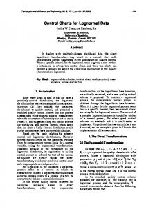
ufacture semiconductors. When using such a process, it is desirable to monitor for a change in the location or scale of the flow width attached to this process. Several samples are taken from the process and the flow width of each is recorded, measured in microns. Some data from such a process is given in Montgomery (2005). First, a reference sample collected before monitoring begins, containing 25 batches taken from the process at 1-hour intervals, each containing 5 measurements. A further 20 batches of 5 measurements are taken after monitoring begins, again at 1-hour intervals. Because our charts do not require a reference sample and can deal with individual observations rather than batches, we view this as constituting a single process with 220 observations. The data is plotted in Figure 1(a). We applied our CvM CPM chart to the output, and the successive values of Wt are plotted in Figure 1(b). From this, we can see there is a change point in the data, which was flagged at data point 199. At this point, Nk,199 was maximized when k = 186, giving a best estimate for the change-point location as ⌧ˆ = 186. We show these estimates superimposed on the data in the above figures.

We now give an example of our CvM chart on a real-world data set. A hard-bake process is used in conjunction with photolithography in order to man-

In applications, we may wish to know not only that a change has occurred but also what is likely to have caused the change. An omnibus detector like ours can detect changes in both location and scale, so signaling a change does not itself tell us whether it is the location or scale that has changed. We will hence consider a basic method of postsignal diagnosis to investigate this. Suppose that the CPM signals a change at time T and estimates the change

(a) Hard-Bake Process

(b) Values of Wt Statistic

Real-Data Application

FIGURE 1. Plot of the Hard-Bake Process Data and the Associated Wt Statistics. The flagged and estimated change point are superimposed as solid and dashed vertical lines, respectively.


Vol. 44, No. 2, April 2012


occurred at ⌧ˆ. We partition the data into the two subsets {X1 , . . . , X⌧ˆ 1 }, {X⌧ˆ , . . . , XT } and then apply simpler two-sample hypothesis tests to these in order to find out the most likely cause of change. For example, to test whether it is the location or scale that is likely to have changed, we apply both a nonparameteric test for location equality and a nonparametric test for scale equality. If the location test gives a lower p-value than the scale test, we conclude that a location shift has occurred, and vice versa.

113

Smirnov. Comparing our CPMs with other state-of-the-art methods showed that our models perform extremely well for detecting shifts in the process mean, being competitive with the Mann–Whitny CPM, while giving far superior performance when the changes involve shifts in the process scale. Comparing our CPMs with the ZEWMA method from Zou and Tsung (2010), we find that, when changes occur after a moderate number of observations have been received, all methods give broadly similar performance for detecting changes to the stream location. However, our methods are superior for detecting decreases in the stream’s scale parameter, while the ZEWMA is better for detecting increases. When the change occurs after a small number of observations, our CPMs are superior to the ZEWMA for detecting all types of changes, except increases in scale.

Here we use the standard Mann–Whitney test (Mann and Whitney (1947)) for location equality and the Ansari–Bradley (Ansari and Bradley (1960)) test for the scale. The p-values for the tests are 5.65⇥10 9 and 1.13 ⇥ 10 2 , respectively. We hence provisionally conclude that the change signal is most likely to have been caused by a location shift in the process, but verifying this conclusively may require further analysis.

Software Implementation

Conclusions

The CPMs described in this paper are implemented in the cpm R package, which can be obtained either from CRAN (http://cran.r-project.org/web/ packages/cpm/index.html) or from the Software section at the first author’s website (http://gordonjross .co.uk).

We introduced two distribution-free change-point models for the purpose of detecting arbitrary changes in an unknown process distribution. A computationally efficient method of computing both models was given, allowing both to be used in Phase II monitoring. Simulation study suggests that the chart based on the Cramer–von-Mises statistic gives better performance than that based on the Kolmogorov– Smirnov statistic, and this chart is also slightly simpler to implement because the mean and standard deviation of the test statistic has an exact functional form. We would therefore recommend the use of the Cramer–von-Mises CPM over the Kolmogorov–

Appendix Table 5 gives the threshold sequences ht corresponding to various choices of the ARL0 for the Cramer–von-Mises and Kolmogorov–Smirnov CPMs. Tables 6, 7, and 8, respectively, provide the standard deviations associated with the mean delays reported in the Experiments section.

TABLE 5. Values of the Threshold Sequence ht that Gives an ARL0 of 200, 370, 500, 1000

Target ARL0 CvM CPM t 20 21 22 23 24 25 26 27

KS CPM

200

370

500

1000

200

370

500

1000

6.5239 6.1624 5.9559 5.7548 5.7150 5.6297 5.6051 5.5780

7.0770 6.7053 6.5451 6.4330 6.3539 6.2648 6.2669 6.2724

7.2457 7.0386 6.7203 6.7867 6.7328 6.5833 6.5510 6.5996

7.6961 7.6776 7.4251 7.3852 7.4136 7.3669 7.3761 7.2357

0.9989 0.9982 0.9983 0.9980 0.9976 0.9973 0.9975 0.9973

0.9993 0.9990 0.9986 0.9987 0.9985 0.9986 0.9988 0.9988

0.9993 0.9993 0.9990 0.9988 0.9990 0.9987 0.9990 0.9989

0.9997 0.9995 0.9995 0.9994 0.9995 0.9994 0.9994 0.9994

Vol. 44, No. 2, April 2012

www.asq.org

114

GORDON J. ROSS AND NIALL M. ADAMS TABLE 5. Continued

Target ARL0 CvM CPM t 28 29 30 30 40 50 60 70 80 90 100 200 300 400 500 600 700 800 900 1000 1500 2000

KS CPM

200

370

500

1000

200

370

500

1000

5.6001 5.5542 5.5674 5.5674 5.5295 5.5163 5.5131 5.5362 5.5437 5.5508 5.5967 5.5735 5.5210 5.6286 5.5354 5.7008 5.7318 5.7515 5.7665 5.7689 5.7723 5.7792

6.2830 6.2707 6.2548 6.2548 6.2877 6.2553 6.3209 6.3575 6.3110 6.3452 6.3615 6.3203 6.4635 6.3092 6.1466 6.3720 6.5082 6.5232 6.5423 6.5392 6.5556 6.5601

6.6193 6.6584 6.5948 6.5948 6.6599 6.6427 6.7078 6.7237 6.7805 6.7037 6.6987 6.7127 6.7808 6.7630 6.6062 6.8209 6.8434 6.8412 6.8572 6.8591 6.8701 6.8793

7.3068 7.3548 7.3543 7.3543 7.4679 7.5856 7.5394 7.5894 7.5838 7.5622 7.6037 7.6276 7.7554 7.6213 7.5865 7.5705 7.5962 7.6213 7.6132 7.6112 7.6398 7.6372

0.9974 0.9975 0.9975 0.9975 0.9973 0.9972 0.9970 0.9968 0.9969 0.9968 0.9968 0.9967 0.9966 0.9961 0.9969 0.9953 0.9970 0.9971 0.9969 0.9972 0.9971 0.9974

0.9986 0.9984 0.9987 0.9987 0.9986 0.9986 0.9986 0.9986 0.9984 0.9985 0.9985 0.9984 0.9983 0.9982 0.9981 0.9983 0.9979 0.9982 0.9981 0.9983 0.9982 0.9983

0.9990 0.9989 0.9991 0.9991 0.9989 0.9989 0.9989 0.9990 0.9989 0.9989 0.9989 0.9988 0.9987 0.9987 0.9987 0.9987 0.9988 0.9987 0.9987 0.9987 0.9988 0.9988

0.9996 0.9994 0.9994 0.9994 0.9994 0.9995 0.9994 0.9994 0.9996 0.9995 0.9995 0.9995 0.9994 0.9994 0.9994 0.9995 0.9994 0.9994 0.9996 0.9995 0.9994 0.9996

TABLE 6. Standard Deviations Associated with the Detection Delays Reported in Table 1 for Location Shifts of Size in Several Distributions

p t(2, 5)/ 5 +

N ( , 1) ⌧

(LN(1, 1/2)

3)/1.6 +

MW

ZEWMA

CvM

KS

MW

ZEWMA

CvM

KS

MW

ZEWMA

CvM

KS

⌧ = 50

1.0 2.0 3.0

12.3 1.74 0.81

118.1 2.1 1.0

14.3 1.8 0.7

30.1 2.3 0.9

3.1 1.1 0.8

4.4 2.0 1.4

3.0 1.0 0.7

3.1 1.1 0.6

7.4 1.2 0.8

40.0 2.7 1.8

6.3 1.2 0.6

6.4 1.1 0.7

⌧ = 300

1.0 2.0 3.0

5.8 1.4 0.7

7.3 2.2 1.0

6.4 1.5 0.7

7.4 1.9 0.8

2.3 0.9 0.7

3.4 1.6 1.1

2.3 0.9 0.7

2.4 0.9 0.6

3.3 0.9 0.6

5.2 2.5 1.6

3.2 0.9 0.5

3.4 0.9 0.6


Vol. 44, No. 2, April 2012


115

TABLE 7. Standard Deviations Associated with the Detection Delays Reported in Table 2 for Scale Shifts of Size in Several Distributions

p t(2, 5)/ 5 +

N ( , 1) ⌧ ⌧ = 50

MW ZEWMA CvM

KS

MW ZEWMA CvM

(LN(1, 1/2) KS 647.9 317.0 96.2 831.4 568.5 293.0

3)/1.6 +

MW ZEWMA CvM

2.0 640.8 3.0 491.1 4.0 434.6 0.5 841.0 0.33 830.8 0.2 832.2

112.1 5.2 2.8 791.6 920.1 636.3

591.8 165.1 28.0 862.5 503.3 172.6

577.2 132.6 21.4 795.1 378.8 118.5

695.2 572.2 495.4 848.8 836.5 829.5

396.3 120.4 40.5 854.6 921.6 886.7

666.6 417.1 160.5 865.4 737.6 395.5

505.1 330.7 261.3 879.1 891.1 893.9

65.4 4.6 2.6 930.7 681.3 361.2

⌧ = 300 2.0 179.4 3.0 59.0 4.0 30.3 0.5 463.1 0.33 443.5 0.2 465.0

6.3 2.7 1.8 724.9 30.9 7.7

39.7 15.7 10.7 43.0 10.0 5.6

36.4 14.3 9.3 46.0 12.8 7.8

279.8 108.4 60.4 537.1 447.5 438.5

22.4 6.6 4.1 774.9 252.9 24.2

69.8 63.5 64.0 22.0 19.6 24.5 13.9 12.4 19.8 160.4 133.0 696.5 17.8 19.9 546.2 9.9 12.1 480.7

4.2 2.2 1.7 248.1 8.8 7.1

KS

375.0 213.6 33.5 18.7 17.4 11.7 788.8 598.0 285.7 138.9 73.5 33.6 25.8 12.2 8.9 22.6 7.2 4.7

20.8 9.9 7.1 16.6 5.7 4.0

TABLE 8. Standard Deviations Associated with the Detection Delays Reported in Table 3 for More General Distribution Shifts

⌧

Change type

MW

ZEWMA

CvM

KS

⌧ = 50

Exp(1) ! Exp(3) Exp(3) ! Exp(1) Gamma(2, 2) ! Gamma(3, 2) Gamma(3, 2) ! Gamma(2, 2) Weibull(1) ! Weibull(3) Weibull(3) ! Weibull(1) Uniform(0, 1) ! Beta(5, 5) Beta(5, 5) ! Uniform(0,1)

19.9 11.4 111.2 80.5 556.1 221.7 545.1 281.3

129.5 26.3 266.9 192.7 800.2 7.7 807.4 15.1

124.9 12.8 123.5 97.3 278.5 88.9 430.0 202.8

126.1 15.9 146.1 120.7 205.8 81.7 346.4 175.5

⌧ = 300


6.0 6.8 13.2 13.5 512.6 33.8 509.2 60.9

8.3 5.3 23.2 15.9 39.6 3.2 239.4 3.9

6.2 7.2 14.5 14.7 13.2 15.6 18.4 22.4

7.0 8.0 16.5 16.7 14.8 14.7 21.4 20.9

References Acosta-Mejia, C. A.; Pignatiello, J. J.; and Rao, B. V. (1999). “A Comparison of Control Charting Procedures for Monitoring Process Dispersion”. IIE Transactions 31, pp. 569–579. Albers, W. and Kallenberg, W. C. M. (2009). “CUMIN Charts”. Metrika 70, pp. 111–130.

Vol. 44, No. 2, April 2012

Anderson, T. W. (1962). “On the Distribution of the TwoSample Cramer–Von Mises Criterion”. Annals of Mathematical Statistics 33, pp. 1148–1159. Ansari, R. A. and Bradley, R. A. (1960). “Rank Sum Tests for Dispersions”. Annals of Mathematical Statistics 31, pp. 1174–1189. Basseville, M. and Nikiforov, I. V. (1993). Detection of

www.asq.org

116


Abrupt Change Theory and Application. Englewood Cli↵s, NJ: Prentice Hall. Buning, H. (2002). “Robustness and Power of Modified Lepage, Kolmogorov–Smirnov and Cramer–von-Mises Two Sample Tests”. Journal of Applied Statistics 29, pp. 907– 924. Chakraborti, S. and van de Wiel, M. A. (2008). “A Nonparametric Control Chart Based on the Mann–Whitney Statistic”. Beyond Parametrics in Interdisciplinary Research: Festschrift in Honor of Professor Pranab K. Sen, pp. 156– 172. Feller, W. (1948). “On the Kolmogorov–Smirnov Limit Theorems for Empirical Distributions”. Annals of Mathematical Statistics 19, pp. 77–189. Gibbons, J. D. (1985) Nonparametric Statistical Inference. New York, NY: McGraw-Hill. Greenwell, R. N. and Finch, S. J. (2004). “Randomized Rejection Procedure for the Two-Sample Kolmogorov–Smirnov Statistic”. Computational Statistics & Data Analysis 46, pp. 257–267. Hackl, P. and Ledolter, J. (1991). “A Control Chart Based on Ranks”. Journal of Quality Technology 23, pp. 117–124. Hawkins, D. M.; Qiu, P. H.; and Kang, C. W. (2003). “The Changepoint Model for Statistical Process Control”. Journal of Quality Technology 35, pp. 355–366. Hawkins, D. M. and Zamba, K. D. (2005). “ A Change-Point Model for a Shift in Variance”. Journal of Quality Technology 37, pp. 21–31. Hawkins, D. M. and Deng, Q. (2010). “A Nonparametric Change-Point Control Chart”. Journal of Quality Technology 42, pp. 165–173. Jensen, W. A.; Jones-Farmer, L. A.; Champ, C. W.; and Woodall, W. H. (2006). “E↵ects of Parameter Estimation on Control Chart Properties: A Literature Review”. Journal of Quality Technology 38, pp. 349–364. Jones-Farmer, L. A. and Champ, C. W. (2010). “A Distribution-Free Phase I Control Chart for Subgroup Scale”. Journal of Quality Technology 42, pp. 373–387.

Kim, P. K. (1969). “On the Exact and Approximate Sampling Distribution of the Two Sample Kolmogorov Smirnov Criterion”. Journal of the American Statistical Association 64, pp. 1625–1637. Mann, H. B. and Whitney, D. R. (1947). “On a Test of Whether One of Two Random Variables Is Stochastically Larger than the Other”. The Annals of Mathematical Statistics 18, pp. 50–60. Montgomery, D. C. (2005). Introduction to Statistical Quality Control. Hoboken, NJ: Wiley. Reynolds, Jr., M. R. and Stoumbos, Z. (2005). “Should Exponentially Weighted Moving Average and Cumulative Sum Charts Be Used with Shewhart Limits?” Technometrics 47, pp. 409–424. Schmid, F. and Trede, M. (1995). “A Distribution Free Test for the Two Sample Problem for General Alternatives”. Computational Statistics and Data Analysis 20, pp. 409– 419. Yeh, A. B.; Mcgrath, R. N.; Sembower, M. A.; and Shen, Q. (2008). “EWMA Control Charts for Monitoring HighYield Processes Based on Non-Transformed Observations”. International Journal of Production Research 46, pp. 5679– 5699. Zamba, K. D. and Hawkins, D. M. (2009). “ Multivariate Change-Point Model for Change in Mean Vector and/or Covariance Structure”. Journal of Quality Technology 41, pp. 285–303. Zhang, J. (2002). “Powerful Goodness-of-Fit Tests Based on Likelihood Ratio”. Journal of the Royal Statistical Society Series B (Methodological) 64, pp. 281–294. Zhou, C.; Zou, C.; Zhang, Y.; and Wang, Z. (2009). “Nonparametric Control Chart Based on Change-Point Model”. Statistical Papers 50, pp. 13–28. Zou, C. and Tsung, F. (2010). “Likelihood Ratio-Based Distribution-Free EWMA Control Charts”. Journal of Quality Technology 42, pp. 174-196.

s


Vol. 44, No. 2, April 2012