Sep 20, 2013 - of Glass is a notable example [11, 15], to which the .... On a different note, and despite the physical appeal of. Thorpe and coworkers ... contains an interpretation of the resulting analytic ex- pressions ..... a cubic equation is obtained, and its solution results in ..... Lect Notes Comput Sc, 2832:78â89,. 2003.
Two rigidity percolation transitions on binary Bethe networks and intermediate phase in glass. Cristian F. Moukarzel
arXiv:1309.5279v1 [cond-mat.dis-nn] 20 Sep 2013
Depto. de F´ısica Aplicada, CINVESTAV del IPN, Av. Tecnol´ ogico Km 6, 97310 M´erida, Yucat´ an, M´exico (Dated: September 23, 2013) Rigidity Percolation is studied analytically on randomly bonded networks with two types of nodes, respectively with coordination numbers z1 and z2 , and with g1 and g2 degrees of freedom each. For certain cases that model chalcogenide glass networks, two transitions, both of first order, are found, with the first transition usually rather weak. The ensuing intermediate pase, although is not isostatic in its entirety, has very low self-stress. Our results suggest a possible mechanism for the appearance of intermediate phases in glass, that does not depend on a self-organization principle. PACS numbers:
I.
INTRODUCTION
Structural (or Graph) Rigidity (SR) [1–5] is the field of applied mathematics that deals with the conditions under which a structure, representable by a graph, can sustain mechanical loads. The rudiments of SR were established by J. C. Maxwell in a classical article [6] that considered the balance of positional degrees of freedom (at the nodes of the graph) and mechanical constraints (edges in the graph). Rigidity, in the context or SR, is the vectorial generalization of connectedness. A graph is connected if it can transmit a current, while it is rigid if it can transmit a force. Connectivity is a particular case of Rigidity, where all nodes have only one degree of freedom (dof) [7]. Among the many applications of SR [8–14], the physics of Glass is a notable example [11, 15], to which the most important applications of the present work pertain. Phillips [16] pioneered the field of SR in Glass, by using constraint counting to explain the observed connection between glass-forming ability and chemical composition in chalcogenides. Thorpe [17] then discussed Phillips’ ideas in the context of Rigidity Percolation (RP). These early works established the bases for the socalled Phillips-Thorpe vector percolation constraint theory [18] of chalcogenide glass, which has in later years received ample support from experiments [19, 20]. In the original version of this theory, constraints are assumed infinitely rigid, as appropriate for T = 0. However, temperature effects, e.g. the fact that links can be broken if the available thermal energy is large enough, can be included in several ways [21, 22]. Within a simple model, temperature effects amount to random link dilution. The models discussed in this work thus have two external parameters: chemical composition, i.e. the relative amount of each atomic species, and link density, loosely representing temperature effects. The original theoretical description of the link between rigidity and glass-forming ability states that, as the chemical composition of a chalcogenide glass is varied, rigidity percolates at a given composition xc , where the system goes from a flexible network to a stressed rigid
one [17, 18]. This critical concentration is, ignoring deviations from Maxwell-Counting, determined by the condition of global constraint balance (GCB), i.e. the composition at which the total number of spatial degrees of freedom equals the total number of mechanical constraints. A more stringent condition, which is not implied by GCB [40], is that of isostaticity, or local constraint balance (LCB). The concept of isostaticity was not part of the early picture for RP in glass, which only discussed GCB. Isostaticity, as a spontaneously organized property of a natural system was first found in sphere packings [12, 23], which are a model for metallic glass. Isostaticity, or LCB, means that not only there is GCB, but that no constraint is redundant. In other words, that constraints are in such way distributed, that none of them is ’wasted’ in an already rigid region, and, therefore, that no degree of freedom is left uncanceled in the system. This delicate balance is never satisfied by systems undergoing random RP, no matter what the density of constraints is. Only those systems satisfy LCB, for which a mechanism for constraint repulsion is at work, that disallows redundant constraints. For sphere packings [12, 23, 24], this mechanism stems form the fact that contact forces must all be compressive, which in turn forbids cycles (overconstrained subgraphs). Thorpe and coworkers [25–27] later proposed an energy-minimization mechanism for constraint repulsion, which appears to be relevant in chalcogenide glasses. Their model predicts the existence of two phase transitions, so it has three phases: floppy, unstressed-rigid, and stressed-rigid. The intermediate phase is composed of varying fractions of an isostatic-rigid phase, with floppy pockets that disappear gradually towards the second transition, as constraints are added to the system. The existence of an intermediate phase in chalcogenides, that appears to be nearly stress-free, had been previously detected by Boolchand [28–31] experimentally. Thorpe and coworkers’ self-organized model [25–27] explains the appearance of the intermediate phase on the grounds that redundant constraints introduce selfstress, and, therefore, increase the elastic energy in the system. Therefore, when the glass is formed, redun-
2 dant constraints would be avoided in order to minimize the energy. However, this line of reasoning might have to be revised in the presence of strong enough external loads acting on the forming glass, as recent work has shown that randomly disordered isostatic networks have zero elastic modulus [32]. Now, the total elastic energy of a rigid network has two parts: one is due to selfstress, and this is effectively minimized for nearly isostatic networks. The second contribution to the elastic energy comes from load-induced stress, and has the form Eload ∼ L2 /B, where L is an external load (e.g. isotropic compression), and B is the elastic modulus that is relevant for that load (e.g. bulk modulus). This contribution is therefore maximized for an isostatic network, according to a recent discussion [32]. Therefore, if the external load is large enough, the total elastic energy might actually be smaller for an overconstrained network than for an isostatic one, under the same set of external conditions. This observation might suggest a possible experimental test of Thorpe et al mechanism for isostaticity, as glass formed under strong enough compression should depart more from isostaticity, i.e. have more self-stress, than glass formed under load-free conditions. Bear in mind, however, that the scale of loads needed to observe this effect in experiments might be too large to be of any relevance. On a different note, and despite the physical appeal of Thorpe and coworkers ideas to explain the genesis of the intermediate phase, it can be seen that, in fact, no selforganization principle or constraint-repulsion mechanism is needed in order to obtain two RP phase transitions and, therefore, an intermediate phase, in a mean-field model of binary chalcogenide networks. The main focus of this work is to study mean-field RP on Bethe networks made from a mixture of two types of sites with different coordination numbers, i.e. a toy model for a binary glass. We will analytically study such “mixed” Bethe networks with arbitrary amounts of random bond-dilution and for arbitrary chemical compositions. It turns out that, under certain conditions, two RP transitions are found (both discontinuous). The ensuing intermediate phase is only isostatic right on the limit with the floppy phase. Nevertheless, it can be argued that this intermediate phase has a low density of redundancies and, therefore, low selfstress. This work is organized as follows. Section II discusses RP on Cayley Trees attached to a rigid boundary. Next in Section III, the analytical methods needed to solve RP on homogeneous Bethe networks without a boundary are reviewed. Section III C discusses how the density of redundant bonds is calculated analytically. Section III C 1 contains an interpretation of the resulting analytic expressions, showing that the system is isostatic at the transition point, while Section III C 2 discusses how this expression is used to locate the true transition point on a Bethe network, and considers some specific examples for which analytic predictions are derived. Section IV generalizes the methods developed in previous sections to the
case of Mixed Bethe networks without chemical order. A specific example is discussed, which displays two RP transitions. Finally, Section V contains a discussion of results, some conclusions, and a perspective for future work.
II.
RP ON CAYLEY TREES
A.
Self consistent equations
Let us first review Central-Force RP on Cayley trees [33] with coordination number z (branching number α = z − 1), where each bond is independently present with probability b. Each node of the tree is assumed to be a rigid object with g degrees of freedom, i.e. at least g independent mechanical constraints acting on it are needed in order to eliminate all its motions. In the following, we will assume g ≥ 2, as g = 1 is usual Percolation [7]. Each present bond acts as a rotatable bar, imposing one mechanical constraint to the degrees of freedom of the two nodes it connects [3]. In a Cayley tree, rigidity stems from the boundary, which itself constitutes layer zero (l = 0) of the tree, and propagates away from the boundary through present links. Let Tl be the probability that an arbitrarily chosen node on layer l be rigidly attached to the boundary, when only its α downwards-pointing links are considered. A node with this property is said to be outwards-rigid (origid). A node in layer (l + 1) will be o-rigid iif it is connected to g or more o-rigid nodes in layer l. Since each of its α links to neighbors on layer l is independently present with probability b, this node will be connected to k o-rigid nodes in layer l with probability � def Pkα (bTl ) = αk (bTl )k (1 − bTl )(α−k) . Therefore, Tl+1 =
α X
Pkα (bTl ).
(1)
k=g
Letting now xl = bTl be the probability that a node in layer l be o-rigid and connected to the node immediately above it on layer (l + 1), one rewrites (1) as xl+1 = b
α X
Pkα (xl ).
(2)
k=g
Far away from the boundary (for l → ∞), xl reaches a fixed point x, that satisfies x=b
α X
Pkα (x) = bSgα (x),
(3)
k=g
Pm where Slm (x) = k=l Pkm (x). This self-consistent equation defines the asymptotic rigid probability T (b) as a
3 function of bond-density b, in the following way [34]: For 0 < x ≤ 1 calculate � T (x) = Sgα (x) (4) b(x) = x/T (x), which together define T (b) implicitly.
B.
Multivaluedness of solutions
Notice that T (b), as given by (4), is multivalued (See red lines in Fig. 1). The trivial solution T = 0∀b is always stable. For b > bCayley two additional solutions exist, one c stable and one unstable. Therefore, for bCayley ≤b≤1 c there are two stable solutions T (b) and therefore a physical criterion is needed to choose the correct one. On a Cayley tree, a well defined procedure exists to determine the appropriate solution, which consists in iterating (1) from a given boundary value T0 . If T0 = 1, equations (1) give rise, for g ≥ 2, to a First-Order Critical RP Transition [33], whereby the order parameter T displays a critical behavior superposed to a first-order jump, above a critical bond density bCayley (See blue line in Fig. 1 for c an example).
III.
RP ON BETHE NETWORKS
A Bethe network has the same local structure as the Cayley tree described in Section II, but has no boundaries. Each node of a Bethe network is connected to z other nodes, without exception. While a tree has no loops (except for those which run through the boundary), any finite Bethe network is bound to have some loops, but those are few in number and can be safely ignored. Many statistical models display the same behavior on Cayley trees with a boundary as they do on Bethe networks without one. For RP this is not the case. It has been shown [35] that the 1st-order critical behavior found for RP on Cayley trees [33] is an artifact due to the excess constraints introduced by the rigid boundary. On a Bethe Network, equations (4) still hold. However, in this case the RP transition is delayed and only happens at a larger b value, becoming a normal first-order one [35], as we review in the following section.
A.
Self-consistent equations
Consider a Bethe network with coordination number z (branching number α = z − 1), and g degrees of freedom per site, where each bond is present with probability b. Choose an arbitrary site i of the network, and let j be a randomly chosen neighbor of i. We will say that j is outwards-rigid (o-rigid for short), if it is rigidly attached to an infinite rigid cluster through outwardspointing links, i.e. those not including the one that con-
nects j to i. Precisely speaking, o-rigidity is not a property of site j, but of site j when considered from neighbor i. This makes o-rigidity a property on the links of a directed graph. However, this consideration is not essential here, and we will continue to refer to o-rigidity as a property of neighboring sites. Now, let T be the probability that a randomly chosen neighbor j of i be o-rigid in the sense above. Notice that j will be o-rigid iif it is connected to g or more origid neighbors, among its α outwards neighbors. Node j is connected to a neighbor that is itself o-rigid, with probability x = bT . Therefore, equation (3) holds for x here as well. A little reflection allows one to conclude that T plays, on Bethe networks, a similar role as on Cayley trees, except for the fact that, on Cayley trees, outwards means “towards the boundary”. Notice that T is not the same as the density R of rigid nodes on the Bethe network. The density R of rigid nodes is found as follows. A site will be rigidly connected to the infinite rigid cluster iif g or more of its z neighbors are o-rigid and connected to it. Therefore R=
z X
(z)
Pj (x),
(5)
j=g
where x = bT , and T , the probability for a neighbor to be o-rigid, satisfies (3). Once T is known, R derives from it trivially using (5), so that its critical behavior derives from that of T . Therefore, we will ignore R and analyze T , in practice regarding it as the “order parameter” of the RP transition, although customarily it is the density R of the infinite cluster what plays that role.
B.
Multivaluedness of solutions
The curve T (b) derived from (4) is multivalued in general, as already discussed for Cayley trees. In the case of Bethe networks, there is no boundary to determine the correct bulk solution by propagation. In order to identify the thermodynamically (globally) stable solution on a Bethe network, one must introduce the concept of redundant constraints and discuss their connection with a free-energy for the RP problem. This has been done in detail previously and we refer the reader to the relevant literature [35] for the conceptual details. For the sake of our work here, it suffices to say that the density of redundant bonds r(b) must satisfy two constraints: Firstly, it must be everywhere continuous. In the second place, whenever multiple (locally) stable solutions exist, the one with the largest r is the thermodynamically (globally) stable one. This second criterion (maximization of r) depends on identifying the number of uncanceled degrees of freedom in the system with a freeenergy for the RP problem. At present, this identification only has the status of a reasonable hypothesis, i.e. one
4 that, having been tested in several instances [34, 35], produces consistent results. However, bear in mind that there is no formal proof of the fact that the number of uncanceled degrees of freedom is the free energy for RP. Establishing this formal connection constitutes one of the most important results still awaiting completion in the field of RP. It turns out that the density of redundant bonds r(p) results from integrating the density of overconstrained bonds, which, in mean-field, is simply T 2 . Therefore, Z p T 2 (b)db. (6) r(b) =
1 0.8
g=2 z=6 T
0.6 0.4 0.2 0 0
0
C.
Exact calculation of redundant bond density 1.
Analytic expression for r
Given that x = bT , one has that T 2 db = T dx − xdT , and therefore Z x(b) Z T (b) r(b) = T dx − xdT. (7) 0
0
The second integral on the r.h.s. is done by parts to obtain Z x x r(b) = 2 T (x)dx − xT |0 . (8) 0
Using (4), the remaining integral can be calculated exactly: Z
dxT (x) =
α Z X j=g
Pjα (x)dx =
α z 1X X z Pj (x) z
(9)
Therefore, α z X 2 X xPjα (x). (j − g)Pjz (x) − z j=g+1 j=g
(10)
0.8
1
0.40 0.30
g=2 z=6 0.20 0.10 0.00 -0.10 0
b)
0.2
0.4 0.6 0.8 Bond Density b
1
FIG. 1: a) Red lines (partially hidden below black and blue ones) indicate the multivalued solution T (b) obtained from equations (4) with 0 ≤ x ≤ 1, for a Cayley tree with g = 2 and z = 6. The entire branch T = 0∀b actually corresponds to a single point x = 0, and is always a locally stable solution. This branch is continued, for x > 0, by an unstable branch with b a decreasing function of x, up to the reversal point bCayley , c where it becomes locally stable, with b an increasing function of x. On a Cayley tree (blue line), a First-Order Critical RP transition happens at bond density bCayley = 0.602789 if c the boundary is perfectly rigid. On a Bethe network with the same g and z the transition happens later (black line), becoming an ordinary First-Order RP transition. The exact location bBethe = 0.656511134 of the transition on the Bethe c network can be determined analytically (See (12)) from the requirement that the density r of redundant bonds (b)) be continuous [35].
z Taking into account that (j + 1)Pj+1 (x) = zxPjα (x), one can also write
k=g j=k+1
z 1 X (j − g)Pjz (x). = z j=g+1
r(x) =
a)
0.4 0.6 Bond Density b
r
This expression was used recently [35] to find r(b) by numerical integration of T 2 (b), while T (b) was calculated by starting from x = 1 and iterating (3), for a given linkdensity b. However, as we now show, r(b) can be calculated analytically with little effort. This will allow us to locate the Bethe RP transition exactly. A similar calculation was done previously [34], but only for the (somewhat simpler) case of Erd˝ os-Renyi graphs. The following section describes how r(b) can be calculated analytically for Bethe networks, starting from (6), and illustrates its use in exactly locating the RP transition with a few simple examples.
0.2
r(x) =
z 1 X (j − 2g)Pjz (x), z j=g+1
(11)
which also defines r(b) implicitly through (4). Expression (11) can be interpreted as follows: Among rigid sites, i.e. those which have g or more rigid neighbors, those with exactly g rigid neighbors contribute no redundant bonds. This is so because sites with exactly g
5 rigid neighbors are isostatically connected to the infinite rigid cluster, and can be removed without altering the rigid properties of the rest of the system. These sites are similar to dangling ends in scalar percolation [36]. Noticing that r is a link-density, by examination of (11) one also concludes that sites with j > g o-rigid neighbors contribute with (j/2 − g) redundancies per site, which is a consequence of the fact that each link is shared by two nodes. In the following, sites with more than g o-rigid neighbors will be called backbone rigid sites. They form the (g + 1)-core contained within the rigid cluster [34]. Notice that (j/2 − g) in (11) is negative unless z ≥ 2g. Since r has to be nonnegative, we conclude that z ≥ 2g is a necessary condition for rigidity on a Bethe network. This is consistent with a simple dof counting argument. On the other hand, rigidity on a Cayley tree only requires z ≥ g + 1, because the boundary provides extra constraints. 2.
Use of r to locate the transition
The continuity requirement for r determines the true transition point on a Bethe network [35] as follows: Below the critical point, the order parameter T , and thus x, are identically zero. The density of redundant bonds is then zero at the critical point, so r(xc ) =
z 1 X (j − 2g)Pjz (xc ) = 0. z j=g+1
(12)
Equation (12) determines xc and, therefore, bc . This can also be written as Pz jPjz (xc ) Pj=g+1 = 2g, (13) z z j=g+1 Pj (xc )
showing that the average number of o-rigid neighbors of a backbone site is exactly 2g at the rigidity transition. This means that, when only backbone sites in the infinite rigid cluster are considered, constraint balance is satisfied at the transition point. Sites which are isostatically connected to the rigid cluster (those with exactly g o-rigid neighbors) also have exact constraint balance because their links are not shared between two o-rigid sites (since they are themselves not o-rigid). We thus conclude that the entire rigid cluster (backbone sites plus isostatically connected sites) satisfies constraint balance at the transition point. This is, of course, just a consequence of the fact that the density of redundancies is zero at the transition point (r(xc ) = 0). However, bear in mind that our calculation neglects finite-size effects, so that r = 0 only means that the number of redundancies is sub-extensive. Clearly, the number of redundancies in the system cannot be exactly zero at the transition point, since a large fraction T 2 of the links are overconstrained there [41]. Now, the precise definition of isostaticity requires that a system be
rigid and have no redundant constraints at all. By a slight abuse of language, we can extend this definition to include systems that are rigid with a sub-extensive number of redundancies. Accepting this extended definition, we can then say that the rigid cluster is isostatic at the transition point in this mean-field system. The general procedure to calculate bc consists in first finding xc from (12), then calculating bc = xc /T (xc ) with T (x) given by (4). For small values of g and z, the roots of (12) can be found analytically. For g = 2 and z = 4, the sum in (12) only contains one term giving rise to xc = 1. This implies T (xc ) = 1 and therefore bc = 1. Thus, a Bethe network with g = 2 and z = 4 is only rigid if undiluted, as discussed already. On the other hand, the Cayley tree with g = 2 and z = 4 can be rigid even in the presence of some small amount of dilution (i.e. bCayley < c 1). For g = 2 and z = 5, the corresponding quadratic equation results in bc = 0.83484234. For g = 2 and z = 6 a cubic equation is obtained, and its solution results in bc = 0.656511134. This last value is consistent with, but more precise than, bc = 0.656, as obtained numerically in previous work [35] with the help of matching algorithms for RP [37, 38]. Notice that bc is slightly smaller than 2/3, which would result for GCB for this case. Fig. 1 shows this last example with g = 2 and z = 6, both for Cayley trees (blue line) and for Bethe networks (black line). The results for Bethe in this figure where obtained by calculating T (x), b(x) and r(x) as given by Eqns. (4) and (11) (red lines), and then choosing as correct solution (black lines) the branch that provides the largest value for r(x). Notice that the density of redundant bonds makes a loop-shaped graph limited by two return points (Fig. 1b, red lines), which correspond to spinodals in the T (b) curve. Actually, one of the two spinodals in the example of Fig. 1 is located at ∞, but the addition of a small field [34] can bring it to finite values of b. The process by which this loop is removed by choosing the branch that maximizes r is a Maxwell construction [35].
IV.
RP ON MIXED BETHE NETWORKS
Although more complex networks can be readily analyzed with the methods developed in this work, the Mixed Bethe Networks (MBN) studied here only have two types ν = 1, 2 of sites. A fraction p1 of the sites has coordination z1 and g1 dof, while the remaining fraction p2 = 1 − p1 has coordination z2 and g2 dof. We will refer to p1 as the “chemical composition” of the network. Consider an undiluted such network with given values of p1 , z1 and z2 . The probability pνρ that a randomly chosen neighbor of a site of type ν be of type ρ depends in general upon the degree to which links between like atoms are favored or disfavored. Under the hypothesis of random bonding, i.e. when all links are equally probable,
6 one has that pνρ only depends on ρ: pνρ =
z ρ pρ def = Pρ , z 1 p1 + z 2 p2
for
1.0
ν, ρ = 1, 2.
0.8
(14)
g1=02 g2=02 z1=04 z2=20
The general case of RP on MBNs with chemical order, i.e. when certain types of links are favored, can also be treated with the methods described in this work, but the mathematics becomes more complicated [42], and will not be discussed in this first presentation. In this work we consider randomly bonded MBNs of the type described above, whose links have been randomly removed, or diluted. For simplicity, we assume homogeneous dilution, i.e. all bonds are present with probability b, no matter what types of sites they link.
0.4 0.2 0.0 0.00
� αρ � X αρ k Tρ = x (1 − x)αρ −k = Sgαρρ (x), k
(15)
k=gρ
where Sgα (x) is the same as defined in (3), and αρ = zρ − 1. The self-consistent equations defining rigidity on an MBN with no chemical order (random bonding) are then T1 = Sgα11 (x) T2 = Sgα22 (x)
(16) (17) def
x = b(P1 T1 + P2 T2 ) = bT.
(18)
Notice that rigidity on randomly-bonded MBNs depends on two parameters: the link density b and the chemical composition p1 . The system’s phase diagram then results from analyzing the average outwards-rigid probability T (b, p1 ) as a function of these two parameters. We will next discuss, in this phase space, trajectories at fixed b (the driving parameter is p1 ) or at fixed p1 (the driving parameter is b). In either case, T can be calculated exactly, as described in the following. 1.
Connectivity b drives the transition
Assume that p1 and p2 = 1 − p1 are given, so we work on MBNs with fixed chemical composition and varying
0.40 0.60 0.80 Bond Density b
1.00
0.04 0.02
Self-consistent equations for rigid probability
Let Tρ , with ρ = 1, 2, be the probability that a neighbor, provided it is of type ρ, be outwards-rigid. An arbitrarily chosen neighbor of a central site, no matter its type, is then outwards- rigid and connected to the central site, with probability x = b(P1 T1 + P2 T2 ). A neighbor of type ρ must in turn have gρ or more o-rigid and connected outwards-neighbors (of any type) in order to be itself outwards-rigid with respect to the central site. Therefore, the outwards-rigid probabilities Tρ of neighbors satisfy
0.20
a)
r
A.
T
0.6
0 g1=02 g2=02 z1=04 z2=20
-0.02 -0.04 0
0.2
b)
0.4 0.6 0.8 Bond Density b
1
FIG. 2: Example of b-driven phase transitions on mixed Bethe networks with g1 = g2 = 2, z1 = 4, and z2 = 20. The “weak” fraction p1 is, from left to right: p1 = 0.12, 0.24, 0.36, . . . , 0.96. a) Average o-rigid probability T , defined by (18), as a function of link-density b. The leftmost case shows two phase transitions. b) Density or redundant links r, as given by (28), as a function of link-density b. Notice the double Maxwell-loop in the rightmost case.
connectivity b. First, from p1 and p2 find P1 and P2 using (14). Then, for 0 ≤ x ≤ 1, calculate T1 = Sgα11 (x) T2 = Sgα22 (x), (19) T = (P1 T1 + P2 T2 ),
and then find b(x) as b=
x x = . (P1 T1 + P2 T2 ) T
(20)
This procedure gives all branches of the eventually multivalued curve T (b) for a given prespecified chemical composition p1 . See red lines in Fig. 2 for an example. The true solution (black lines in Fig. 2) is determined by the continuity of the density of redundant bonds r, as discussed in Section IV C. 2.
Chemical composition p1 drives the transition
In this case we assume b to be known, i.e. work on graphs with fixed dilution and varying chemical compo-
7 1.0
1.0
0.8
0.8
g1=02 g2=02 z1=04 z2=20
0.6
g1=02 g2=02 z1=04 z2=20
T
0.6 T
0.4
0.4
0.2 0.0 0.00
0.2 0.20
0.40
0.60
0.80
1.00
p1
a)
0.0 0.6
0.7
0.8 0.9 Bond Density b
1
0.7
0.8 0.9 Bond Density b
1
a)
0.1
1.0
r
0.8 0 T1, T2
g1=02 g2=02 z1=04 z2=20
-0.1 0
0.2
0.4
0.6
0.8
0.4 0.2
1
p1
b)
0.6
0.0 0.6
b) 0.06
g1=02 g2=02 z1=04 z2=20 0.03 r
FIG. 3: Example of p1 -driven phase transitions on mixed Bethe networks with g1 = g2 = 2, z1 = 4, and z2 = 20. The link-density is, from left to right: b = 0.2, 0.3, 0.4, . . . a) Average o-rigid probability T , defined by (18), as a function of chemical composition p1 . Double phase transitions, which happen for b ≈ 0.85 are not seen in this figure. They are displayed in detail in Fig. 5. b) Density or redundant links r, as given by (28), as a function of chemical composition p1 .
0
sition p1 . For 0 ≤ x ≤ 1 we first calculate: � T1 = Sgα11 (x) T2 = Sgα22 (x),
c)
and then use (18) in the form x/b − T2 P1 = , T1 − T2
(22)
to find P1 (x). From P1 one can find the chemical composition, which is given by p1 = P1 z2 /(z2 P1 + z1 (1 − P1 ))
-0.03 0.6
(21)
0.7 0.8 0.9 Bond Density b
1
FIG. 4: Zoom of double phase transitions in the b-driven case, on mixed Bethe networks with g1 = g2 = 2, z1 = 4, and z2 = 20. The “weak” fraction p1 is, from left to right: p1 = 0.940, 0.945, 0.950, . . . , 0.980 a) Average o-rigid probability T , defined by (18). b) o-rigid probabilities for each of the components. c) Density or redundant links r, as given by (28).
(23)
This procedure gives all branches of the eventually multivalued curve T (p1 ), i.e. rigidity as a function of chemical composition, for a given prespecified bond dilution b. See red lines in Fig. 3 for an example. The true solution (black lines in Fig. 3) is determined by the continuity of the density of redundant bonds r, as discussed in Section IV C.
B.
Redundant bonds in mixed-coordination Bethe networks
As discussed in recent work [35], in order to find the density r of redundant links we need to integrate the density of overconstrained links (as done in Section III C
8 1.0 0.8 0.6 T
g1=02 g2=02 z1=04 z2=20
0.4
a)
(24)
Using (14), the density of overconstrained bonds that has to be integrated in order to obtain the density of redundant bonds is then
0.2 0.0 0.95
easily show that X12 = P1 p12 + P2 p21 X11 = P1 p11 X22 = P2 p22 .
0.96 p1
0.97
X11 T12 + X12 T1 T2 + X22 T22 = (P1 T1 + P2 T2 )2 = T 2 .(25) Therefore,
1.0
r=
T1, T2
0.8 0.6 0.4 0.2 0.0 0.95
b)
0.96 p1
0.97
0.008 g1=02 g2=02 z1=04 z2=20
r
0.004
0.000
Z
b
T 2 db,
(26)
0
which looks exactly the same as (6), but bear in mind that, here, T is given by (18), i.e it is the average of T1 and T2 with weights P1 and P2 . The simplicity of (26) is a consequence of the random-bond hypothesis. While the case of chemical order will not be considered here, we can anticipate that, whenever the network has chemical order, the density of overconstrained links no longer equals T 2 . In other words, for a network with chemical order, the probability for a randomly chosen link to be overconstrained is not simply the product of the a-priori probabilities that its end sites be outwardsrigid (which is T for each site). Now, since x = bT (Eq. (18)), and, following the same steps as in Section III C 1, one has Z x x T (x)dx − xT |0 = r = 2 0 � � Z x � � Z x x x T2 dx − xT2 |0 . T1 dx − xT1 |0 + P2 2 = P1 2 0
0
(27) 0.95
c)
0.96 p1
0.97
FIG. 5: Zoom of double phase transitions in the p1 -driven case, on mixed Bethe networks with g1 = g2 = 2, z1 = 4, and z2 = 20. The link-density b is, from left to right: b = 0.830, 0.835, 0.840, . . . , 0.865. a) Average o-rigid probability T , defined by (18). b) o-rigid probabilities for each of the components. c) Density or redundant links r, as given by (28).
Using (15) and (11), this can be written as r =
z1 z2 P1 X P2 X (j − 2g1 )Pjz1 (x) + (j − 2g2 )Pjz2 (x), z1 j=g +1 z2 j=g +1 1
2
(28) which equals the average of the redundant-link density rρ for each homogeneous system (See (11)), with weights Pρ . C.
for Bethe Networks). A link or bond is overconstrained whenever both its end sites are outwards-rigid. A bond that connects a site of type ρ to a site of type ν is therefore overconstrained with probability Tρ Tν . If a fraction Xνρ of all links connect sites of type ν to sites of type ρ, the average density of overconstrained links is X11 T12 + X12 T1 T2 + X22 T22 . On the other hand, one can
Continuity of r
Whenever there are multiple stable solutions for T (b, p1 ), the ambiguity is raised by requiring that r be maximal and a continuous function of the parameter that drives the transition (either b or p1 ). This is done by comparing the values of r (Eq. (28)) for the various branches with the help of either (20) or (23).
9 The resulting final rigidity probabilities T are shown in Fig. 2 for fixed p1 and varying b, and in Fig. 3 for fixed b and varying p1 . In both cases one finds instances where two RP transitions exist, for certain ranges of parameters. These ranges turn out to be rather narrow for the cases displayed in Figs. 2 and 3, which correspond to g1 = g2 = 2, z1 = 4, and z2 = 20. In fact it is easier to find double transitions when there is both coordination contrast and dof contrast, but we chose to analyze a case with g1 = g2 and only coordination contrast, because this is similar to what happens in chalcogenide glass, where all atoms have the same number of dof (six in three dimensions). The connectivity range in which two p1 -driven RP transitions occur is indeed so narrow that it is not observed in Fig. 3. In order to more clearly appreciate the double transitions, we have made dedicated plots which show the double transitions in more detail. Figures 4 and 5 show zoomed-in plots of the double transitions, respectively for the b-driven and p1 -driven cases. The plots of r (Figures 4c and 5c) show that, associated with double transitions, there are two successive Maxwell loops in r. Several observations can be done regarding the intermediate phase, or first rigid phase, for this example: 1) The intermediate phase, as already discussed in Section III C 2 is isostatic right at the transition from the floppy phase. 2) The density r or redundant constraints is rather small in the intermediate phase, much smaller than in the second rigid phase. A similar observation can be done regarding the density T 2 of overconstrained links. 3) In the intermediate phase T2 ≈ 0.9 while T1 ≈ 0.2 (See Figures 4b and 5b), so that the strong component (sites with coordination z2 = 20) rigidizes much more than the weak component (sites with z1 = 4). At the second phase transition, where the second rigid phase starts, the weak component rigidizes abruptly, from T1 ≈ 0.2 to T1 ≈ 0.8, while the jump in T2 is there almost unnoticeable. Therefore, although both components suffer discontinuities in T at both transitions, in practice one can say that the strong component 2 rigidizes at the first transition, while the weak component 1 does so only at the second transition. In the intermediate phase, the density of overconstrained links T 2 is rather small of the order of 0.1, while it becomes of around 0.6 at the second transition. Therefore, the intermediate phase obtained in this model is rigid and, although not isostatic, it is practically stressfree compared to the second rigid phase.
V.
DISCUSSION
We have presented an analytical study of Rigidity Percolation (RP) on randomly bond-diluted (link density b) Bethe networks made from a binary mixture of sites, respectively with fractions p1 and p2 , coordination numbers z1 and z2 , and having g1 and g2 degrees of freedom (dof) at each site. Bond dilution can be thought of as representing temperature effects in an approximate way.
While chemical order, i.e. preferential bonding or dilution, can also be studied with the methods discussed here, in this work only random bonding (no chemical order) and homogeneous dilution was analyzed. Our main result is that, for certain parameter combinations, two RP phase transitions, either b-driven or p1 -driven, are found. A previous numerical study by Thorpe and coworkers on a related problem (in [11]), found no evidence of two phase transitions. A key step in this study was the calculation of the density r of redundant links, which results from integrating the density T 2 of overconstrained links, as given by Eq. (6). In previous work on homogeneous Bethe networks [35], this integral was done numerically, while T was found by iterating (1). In contrast to this, we have shown that Eq. (6) can be explicitely integrated, so that r can be calculated analytically, resulting in Eq. (11) for homogeneous Bethe networks, and (28) for mixed Bethe networks. For homogeneous networks, having an analytical expression for r allows one to determine the transition point exactly (Eq. (12)) for a few simple examples, and our results are in good agreement with previous numerical work [35]. An analysis of the transition-point equation in the form of Eq. (13) furthermore allows one to conclude that, right at the transition, the rigid cluster is isostatic, i.e. satisfies constraint balance. On mixed Bethe networks it is found that, for certain combinations of parameters, two RP phase transitions instead of one, are found. The resulting intermediate phase is usually rather narrow. It is easier to obtain double transitions for networks with g1 6= g2 and z1 6= z2 , i.e. both coordination contrast and dof contrast. However, in this analysis we concentrated on showing that a model binary glass, with g1 = g2 = 2 and z1 6= z2 , shows two transitions. Fixing z1 = 4, which is the minimum required to obtain a rigid structure when g = 2, we find that z2 = 16 is the minimum required coordination of the “strong” component, in order to obtain two RP transitions. However, in this case the intermediate phase is extremely narrow, so we chose to analyze z2 = 20 instead, since its intermediate phase is stronger. Figs. 2 and 3 show, respectively, the b-driven and the p1 driven transitions for a broad range of parameters, while Figs. 4 and 5 concentrate on those cases for which an intermediate phase exists. The intermediate phase is only isostatic at one of its endpoints, but it can be argued that its self-stress is everywhere rather low, compared to that of the second rigid phase. Furthermore, we have observed that, approximately speaking, the strong component rigidizes abruptly at the first transition (T2 jumps form zero to a large value) , while the weak one only does so at the second transition, remaining only very weakly rigid (T1 is small) in the intermediate phase. Our results, therefore, suggest an alternative mechanism for the appearance of an intermediate phase in glass, which does not derive from a self-organization principle but is a consequence of the heterogeneity in the proper-
10 ties of the components forming the network. Although the resulting intermediate phase is not isostatic, it can be argued that its self-stress is very low compared to that of the second rigid phase. Notice that available experimental results on glass point to the existence of an intermediate phase with low stress but they cannot determine whether this phase is rigorously isostatic or not. Thorpe et al [25–27], on the other hand, explain the intermediate phase as being a consequence of self-stress minimization. Their proposed mechanism would give rise to an isostatic intermediate phase, even on networks made from a single component. We have noted that selfstress minimization does not necessarily mean elasticenergy minimization, as the elastic modulus of nearly isostatic structures is very low. Therefore, under strong enough pressure, an isostatic structure would in fact maximize the total elastic energy. This observation suggests a possible experimental test of the proposed isostatic properties of the intermediate phase. Clearly, self-organization a la Thorpe et al, can be included in a model as the one discussed here [39], and it would be interesting to see what results from the inter-
play of two different mechanisms giving rise to multiple phase transitions. An important ingredient that is still lacking in our present analysis is chemical order, i.e the fact that different atoms bond preferentially to atoms of the same or a of a different species. The introduction of chemical order is at present work in progress. Chemical order complicates the treatment slightly, but appears feasible nevertheless. Numerical studies intended to corroborate the results presented in this work are under way, and will be published elsewhere. Apart from mixed Bethe networks, of course it is of interest to analyze numerically threedimensional models of chalcogenide glass, in order to verify if the mechanism for intermediate phase described here is still valid for more realistic cases.
[1] L. Asimow and B. Roth. Rigidity of graphs. Trans. Am. Math. Soc., 245:279–289, 1978. [2] L. Asimow and B. Roth. Rigidity of graphs .2. J. Math. Anal. Appl., 68:171–190, 1979. [3] H. Crapo. Structural rigidity. Struct. Topol., 1:26–45, 1979. [4] L. Lovasz and Y. Yemini. On generic rigidity in the plane. Siam J Algebra Discr, 3:91–98, 1982. [5] W. Whiteley. Infinitesimally rigid polyhedra .1. statics of frameworks. Trans. Am. Math. Soc., 285:431–465, 1984. [6] J. C. Maxwell. Constraint counting. Philos Mag ER, 27:294, 1864. [7] C. Moukarzel and P. M. Duxbury. Comparison of rigidity and connectivity percolation in two dimensions. Phys. Rev. E, 59:2614–2622, 1999. [8] S. Feng and P. N. Sen. Percolation on elastic networks - new exponent and threshold. Phys. Rev. Lett., 52:216– 219, 1984. [9] W. Whiteley. A correspondence between scene analysis and motions of frameworks. Discret Appl. Math., 9(3):269, 1984. [10] C. Moukarzel and P. M. Duxbury. Stressed backbone and elasticity of random central-force systems. Phys. Rev. Lett., 75:4055–4058, 1995. [11] M. Thorpe and P. M. Duxbury, editors. Rigidity Theory and Applications. Fundamental Materials Research. Kluwer Academic & Plenum Press, New York, 1999. [12] C. Moukarzel. Granular matter instability: a structural rigidity point of view. In Rigidity Theory and Applications, Fundamental Materials Science, page 125, New York, 1999. Plenum Press. [13] A. J. Rader, B. M. Hespenheide, L. A. Kuhn, and M. F. Thorpe. Protein unfolding: Rigidity lost. Proceedings Of The National Academy Of Sciences Of The United States Of America, 99:3540–3545, 2002.
[14] A. R. Berg and T. Jordan. Algorithms for graph rigidity and scene analysis. Lect Notes Comput Sc, 2832:78–89, 2003. [15] J. C. Mauro. Topological constraint theory of glass. Am. Ceram. Soc. Bull., 90:31–37, 2011. [16] J. C. Phillips. Topology of covalent non-crystalline solids .1. short-range order in chalcogenide alloys. J. NonCryst. Solids, 34(2):153, 1979. [17] M. F. Thorpe. Continuous deformations in random networks. J. Non-Cryst. Solids, 57(3):355, 1983. [18] J. C. Phillips and M. F. Thorpe. Constraint theory, vector percolation and glass-formation. Solid State Commun., 53(8):699, 1985. [19] D. R. Swiler, A. K. Varshneya, and R. M. Callahan. Microhardness, surface toughness and average coordinationnumber in chalcogenide glasses. J. Non-Cryst. Solids, 125(3):250, November 1990. [20] P. Boolchand, R. N. Enzweiler, R. L. Cappelletti, W. A. Kamitakahara, Y. Cai, and M. F. Thorpe. Vibrational thresholds in covalent networks. Solid State Ion., 39:81– 89, 1990. [21] G. G. Naumis. Energy landscape and rigidity. Physical Review E, 71:026114, 2005. [22] P. K. Gupta and J. C. Mauro. Composition dependence of glass transition temperature and fragility. i. a topological model incorporating temperature-dependent constraints. Journal Of Chemical Physics, 130:094503, 2009. [23] C. F. Moukarzel. Isostatic phase transition and instability in stiff granular materials. Phys. Rev. Lett., 81:1634– 1637, 1998. [24] C. F. Moukarzel. Response functions in isostatic packings. In Haye Hinrichsen and Dietrich E. Wolf, editors, The Physics of Granular Media, pages 23–43. WileyVCH, Berlin, 2005. [25] M. F. Thorpe, D. J. Jacobs, M. V. Chubynsky, and
Acknowledgments
The author acknowledges financial support from Conacyt under SNI program.
11
[26]
[27] [28]
[29]
[30] [31]
[32] [33]
J. C. Phillips. Self-organization in network glasses. J. Non-Cryst. Solids, 266:859–866, 2000. M. F. Thorpe, M. V. Chubynsky, D. J. Jacobs, and J. C. Phillips. Non-randomness in network glasses and rigidity. Glass Phys. Chem., 27:160–166, 2001. M. V. Chubynsky and M. F. Thorpe. Self-organization and rigidity in network glasses. Curr. Opin. Solid State Mat. Sci., 5:525–532, 2001. D. Selvanathan, W. J. Bresser, P. Boolchand, and B. Goodman. Thermally reversing window and stiffness transitions in chalcogenide glasses. Solid State Commun., 111(11):619, 1999. D. Selvanathan, W. J. Bresser, and P. Boolchand. Stiffness transitions in sixse1-x glasses from raman scattering and temperature-modulated differential scanning calorimetry. Phys. Rev. B, 61:15061–15076, 2000. Y. Wang, P. Boolchand, and M. Micoulaut. Glass structure, rigidity transitions and the intermediate phase in the ge-as-se ternary. Europhys. Lett., 52:633–639, 2000. P. Boolchand, X. Feng, and W. J. Bresser. Rigidity transitions in binary ge-se glasses and the intermediate phase. J. Non-Cryst. Solids, 293:348–356, 2001. C. F. Moukarzel. Elastic collapse in disordered isostatic networks. Europhys. Lett., 97:36008, 2012. C. Moukarzel, P. M. Duxbury, and P. L. Leath. Firstorder rigidity on cayley trees. Phys. Rev. E, 55:5800–
5811, 1997. [34] C. F. Moukarzel. Rigidity percolation in a field. Phys. Rev. E, 68:056104, 2003. [35] P. M. Duxbury, D. J. Jacobs, M. F. Thorpe, and C. Moukarzel. Floppy modes and the free energy: Rigidity and connectivity percolation on bethe lattices. Phys. Rev. E, 59:2084–2092, 1999. [36] D. Stauffer and A. Aharony. Introduction to Percolation Theory. Taylor and Francis, Bristol, 2nd. edition, 1994. [37] C. Moukarzel. An efficient algorithm for testing the generic rigidity of graphs in the plane. J. Phys. A-Math. Gen., 29:8079–8098, 1996. [38] D. J. Jacobs and B. Hendrickson. An algorithm for twodimensional rigidity percolation: The pebble game. J. Comput. Phys., 137(2):346, NOV 1 1997. [39] J. Barre, A. R. Bishop, T. Lookman, and A. Saxena. Adaptability and ”intermediate phase” in randomly connected networks. Phys. Rev. Lett., 94:208701, 2005. [40] Despite wrong claims in numerous recent articles, where GCB=isostaticity is explicitely stated. [41] However, this does not necessarily imply that the number of redundancies is large. A single redundant link may be enough to make a large number of links overconstrained. [42] C. Moukarzel to be published.