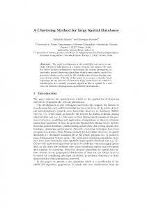
Dec 21, 2017 - Steve Oudotd,Kathryn Hessc,and Cathrin Briskena a Swiss Institute ...... Let X be a topological space and let f : X â R be a Morse-type function.
Two-Tier Mapper: a user-independent clustering method for global gene expression analysis based on topology Rachel Jeitzinera , M athieu Carri`ered , Jacques Rougemontb , Steve Oudotd , Kathryn Hessc , and Cathrin Briskena a Swiss Institute for Experimental Cancer Research,
arXiv:1801.01841v1 [q-bio.GN] 21 Dec 2017
b Bioinformatics and Biostatistics Core facility, c Brain and Mind Institute, School of Life Sciences, Ecole Polytechnique F´ ed´ erale de Lausanne, CH-1015 Lausanne, Switzerland d INRIA Saclay France There is a growing need for unbiased clustering methods, ideally automated. We have developed a topology-based analysis tool called Two-Tier Mapper (TTMap) to detect subgroups in global gene expression datasets and identify their distinguishing features. First, TTMap discerns and adjusts for highly variable features in the control group and identifies outliers. Second, the deviation of each test sample from the control group in a high-dimensional space is computed and the test samples are clustered in a global and local network using a new topological algorithm based on Mapper. Validation of TTMap on both synthetic and biological datasets shows that it outperforms current clustering methods in sensitivity and stability; clustering is not affected by removal of samples from the control group, choice of normalization nor subselection of data. There is no user induced bias because all parameters are data-driven. Datasets can readily be combined into one analysis. TTMap reveals hitherto undetected gene expression changes in mouse mammary glands related to hormonal changes during the estrous cycle. This illustrates the ability to extract information from highly variable biological samples and its potential for personalized medicine.
1
Introduction
Large datasets are generated at an exponentially increasing pace in biology and medicine, while the development of tools to analyze these data is lagging behind. The high variability of biological, in particular human, samples poses a challenge. It takes large sample numbers to understand the distribution of the data and to extract statistically significant features [16]. Often the choice of normalization is ambiguous and this affects the outcome of the analysis [16].
Topology is a field of mathematics devoted to the study of shapes. Topological data analysis (TDA) is used to reduce dimensions and to recognize patterns ([4], [10]). Global gene expression data samples for instance are considered as point clouds in a high-dimensional space. Topological methods can transform them into networks; the nodes are clusters of samples and the edges are determined by common samples between nodes [24]. Analysis of such networks enables discovery of specific patterns in any dataset. As topology is not sensitive to scale it is useful for highly variable biological data.
1
TDA approaches have been applied to numerous scientific domains including biology ([10]). A clustering method based on algebraic topology, Mapper, [24] has been applied to analyze large biological datasets, such as global gene expression profiles [26], temporal single-cell RNA-seq data [31], and genomic data of viral evolution [8]. For the global gene expression analysis [14], [9], [3], the data were pre-processed with a statistical tool and the combination of this statistical tool and Mapper is called Progression Analysis of Disease (PAD). Since the outcome of several statistical method, depending for the case of PAD on linear regression, can be strongly affected by outliers in both the control and the test group [28], [21], large sample numbers are critical for the method to render reliable results [34]. Finding the outliers and removing them is troublesome in small datasets, where the definition of outliers is arbitrary [34],[23].
Like other clustering methods such as k-means [20], PAD, as well as Mapper alone, and hierarchical clustering depend on parameters the user choses; modifying parameters changes the output significantly [35]. Finally, clustering methods such as k-means do not verify stability results: small perturbations in the dataset can lead to different clusters and different conclusions [21].
Here, we present a topology-based method inspired by PAD for global gene expression analysis particularly suited for small sample numbers (n < 25), called Two-Tier Mapper (TTMap) which identifies significant variation and relatedness in datasets and i) can be used in a paired analysis, ii) takes into account batches, iii) is stable, and iv) does not require the user to choose any parameters.
2
Results
2.1
Method description
2.1.1
Overview
Each global gene expression profile represents a high dimensional vector in Rn with n the number of genes. The input (Fig 1 a, green) of Two-Tier Mapper (TTMap) is given by two matrices in log-2 scale, one for the control samples N the other for the test samples T. Batches are defined as groups of samples distinguished by technical variation such as date and site of analysis, technical platform used or biological disparity such as different strains of mice.
TTMap comprises two independent parts, the Hyperrectangle Deviation Assessment (HDA) and the Global-toLocal Mapper (GtLMap). The first characterizes the control group and adjusts for outliers yielding the corrected control group that serves as a reference to calculate the deviation of each test vector individually. The second part uses the Mapper algorithm [32] where the parameters were carefully chosen; a two-tier cover, a special distance and an automated parameter of closeness. The two-tier cover detects global and local differences in the patterns of deviations thereby capturing the structure of the test group. The test samples are clustered according to the
2
shape of their deviation. The extent of deviation of individual clusters translates into a color-code. A list of the differentially expressed genes is also provided (Fig 1 a) (Details in Online Methods).
2.1.2
Hyperrectangle deviation assessment (HDA)
Hyperrectangle deviation assessment (HDA) compares the value of each feature of any control sample N to the others in the same batch of the group N (Fig 1 a, ”adjustement of control group”). If the difference in absolute value is further than e, a parameter computed using the variances of all the genes (Online methods), from the median of the others, it is considered an outlier and replaced by Not a Number (NA). The numbers of replaced values in each sample in the control group (Fig 1 a, shown by N ∗ ) are represented as a barplot (Fig 1 b). This allows the user to discern outlier samples for standard statistical analyses and to identify highly variable features of the control group (Fig 1 b). Thus, HDA creates a matrix that describes the range of expression values expected in group N corrected for outliers. The (k, j)-coefficient of this matrix of the corrected control group, (N k )j , which corresponds to the j th feature of sample k, is computed by:
((N )k )j =
N A
if |(Nk )j − mediani∈I (Nk ),i6=k (Ni )j | ≥ e
(N ) k j
otherwise.
,
Here, (Ni )j denotes the value of the expression of gene j in sample i, and I (Nk ) ⊆ {1, . . . , S} is the set of indices of control samples in the batch containing Nk . NAs are replaced by the median of the normal values in their batch.
Each feature has a range of values, in which control measurements are expected, for sample Tk and gene j given by Bjk =
�
� min (N i )j , max (N i )j ,
i∈I (Tk )
i∈I (Tk )
where I (Tk ) is the set of indices of control samples in the batch containing Tk . For each batch, these normal ranges determine a hyperrectangle in n-dimensional space Bk = B1k × · · · × Bnk (Fig 1 c: example with n = 2). Each test sample Tk is decomposed as Tk = N c.Tk + Dc.Tk , where N c.Tk is the normal component, which is its projection onto the hyperrectangle Bk and hence is the closest point to Tk inside Bk (Fig 1 c) and the deviation component (Dc.Tk ), which is the remainder of the projection (Fig 1 c) (Online Methods)
More precisely, for each test sample Tk and feature j, HDA computes x ¯kj ∈
�
� min (N i )j , max (N i )j ,
i∈I (Tk )
i∈I (Tk )
such that |(Tk )j − x ¯kj | ≤ |(Tk )j − x| for all x∈
�
� min (N i )j , max (N i )j .
i∈I (Tk )
i∈I (Tk )
3
Then, (N c.Tk )j = x ¯kj
for all 1 ≤ j ≤ n
and (Dc.Tk )j = (Tk )j − (N c.Tk )j
2.1.3
for all 1 ≤ j ≤ n.
Global-to-Local Mapper (GLMap)
The second step of TTMap first calculates distances and provides a visualization of these distances and relations in the dataset, in a manner analogous to Mapper [24]. It forms bins according to a measure of similarity on the test vectors.
The default similarity measure in GLMap is the mismatch distance, dM given by a sum of mismatches, where a mismatch is defined by a gene that is differentially expressed in opposite direction as measured by the deviation component (Online Methods, Fig 1 d, n=1). The deviation must be bigger than α to avoid counting noise as mismatch. The mismatch distance, or sum of mismatches is defined as follows (Fig 1 d), for a fixed α ≥ 0 dM (X, Y ) =
n X
dm ((Dc.X)i , (Dc.Y )i ), where
i=1
dm (x, y) =
0 1 |x−y| 8αn
if sign(x) = sign(y), if sign(x) 6= sign(y)
.
and |x| or |y| ≥ α otherwise
If features measured are gene expression values, then the default value does not need to be changed and is set to α = 1, corresponding to a 2-fold-change, which is a standard cut-off for gene expression.
Furthermore, GLMap uses a filter function, given by properties of interest of the samples. It can be chosen by the user to take into account relevant variables, such as the age of the patients in a cohort. The default filter function in GLMap, called total absolute deviation and denoted τ , measures the overall deviation of a test vector from the control, i.e., τ : T → R : Tk 7→
X
| (Dc.Tk )l |,
l∈S
where S is a subset of features, determined by the user, the default being to select all features, and T is the set of test vectors, which is a subset of Rn . Let Im τ denote the image of τ with multiplicity, i.e., Im τ = {(τ (X), σ) | X ∈ T, σ ∈ {1, . . . , mult(X)}} ⊆ R × N, with the lexicographic order, where mult(X) = card(τ −1 (τ (X))) is the multiplicity of τ (X) and for any 0 ≤ a < b ≤ 100, let q[a,b[ = π1
�
� y ∈ Im τ | quantilea (Im τ ) ≤ y < quantileb (Im τ ) , 4
where π1 is the natural projection on the first component, and quantilea (Im τ ) is the a-th quantile of the ordered values in Im τ .
In default mode, GLMap applies the Mapper algorithm [24] to the quadruple given by the mismatch distance dM , a closeness parameter � (computed from the data ,Online Methods, which depends on the variance in the control group), the total absolute deviation τ , and the covering of Im τ given by I = {Im τ, q[0,25[ , q[25,50[ , q[50,75[ , q[75,100] }. This means that GLMap performs single-linkage clustering with parameter dM , i.e. two samples X and Y are clustered together if and only if there is a list of samples X = X0 , X1 , ..., Xn = Y such that dM (Xi , Xi+1 ) < � for all 0 ≤ i ≤ n − 1 to • all of T, giving the connected components {C01 , . . . , C0l(0) } of the graph G� defined by the vertex set {Tk } and the edge set {(Ta , Tb ) s.t. dM (Ta , Tb ) < �} and then to • the pre-image with respect to τ of each of the quantiles q0,25 , q25,50 , q50,75 , and q75,100 , which gives the connected components {Ci1 , . . . , Cil(i) } of the subgraph G� (i) = τ −1 (Ii ), where Ii ∈ I. Two connected components Cij and Ckl are represented as spheres with diameters increasing with the number of samples in each component. The spheres are connected by an edge whenever Cij ∩ Ckl 6= ∅, i.e. the algorithm links clusters that share samples as every sample is assessed twice for connectivity, once globally and once within its quartile, links are formed between local and global structures, enabling the discovery of subgroups based on the filter function of the global clusters (Fig 1 a, Part2).
The color of a sphere in the output figure of the method (see example in section 2.4, Figure 3 a) is determined by the average of the values of the filter function applied to the samples in the bin. A legend for the color code is provided at the bottom of the output figure, for the size of the balls on the right, and for the different tiers on the left, i.e. the overall clustering and the clustering in the different quartiles, (Fig 1 a, Part2). A list of the differentially expressed genes per cluster is provided.
2.2
Theoretical aspects
To assess the theoretical stability of TTMap, the effect of modifications of the source space, of the filter function and of approximations with a point cloud on its outputs was studied (Online methods). Since there is no natural distance on the outputs of TTMap, one can not assess the stability directly on the TTMap graphs. Therefore, the information contained in the TTMap graphs is summarized as a diagram in R2 (Supplementary Fig S4 d), similar to a persistence diagram (PD) [17], where there is a natural distance d that generalizes the distance on PD, allowing a comparison of TTMap graphs. The PD are summaries of the topological features of the graph (connected component, hole, branch, etc...) depicted as dots. Here, we supplemented PD with links between the “local” features and the connected components
5
(or the global clusters), forming a descriptor, denoted DM (X, f, I), for a space X and a filter function f : X → R that verifies mild regularity conditions. In terms of these enriched PD, we establish the following theorems, stated informally here and precisely in the Online Methods in Theorem 4.2,4.4,4.5, 4.6 respectively. • Completeness The descriptor is complete, i.e., from the diagram DM (X, f, I) the information contained in the graph of T T M ap(X, f, I) can be recovered. • Stability with respect to changes of the filter function If the filter function f on the space is perturbed, the distance between the diagrams of f and of its perturbation is not greater than the amount of perturbation. • Stability with respect to perturbations of the domain If the starting space X is perturbed, then the distance between the diagrams of X and of its perturbation depends linearly on the amount of perturbation. • Stability with respect to point cloud approximations If data points are sampled on a space X, then the difference between the diagrams associated to X and to the δ-neighborhood graph built on the point cloud is less than a value depending on δ.
2.3
In silico validation
TTMap was tested on simulated data that mimics a situation for which standard methods are weak, i.e., small sample size (n> S, and if the probabilities accumulated around 0 as is the case for gene expression data, then the sum over all genes of mismatches follows a Poisson distribution with Pn mean j=1 (Pkl )j . This in turn allows one to determine how significant the number of mismatches between Pn X and Y is, if both vectors follow the same distribution. Hence, � is given by P ( j=1 (Pkl )j < �) = β, which can be obtained from the quantiles of a Poisson law. Thus, samples are linked if the number of mismatches between them is less than �, which is the β% confidence threshold of mismatches for samples following the same distribution. If � is chosen such that P (
Pn
l j=1 (Pk )j
< �) = 0.025, it means that only in 2.5% of the cases if Xk and Xl are dis-
tributed in the same way, they would have such a small number of mismatches and therefore it is certain that Pn Xk and Xl must be clustered together. In the same way, if � is chosen such that P ( j=1 (Pkl )j < �) = 0.975, it means that only in 97.5% of the cases if Xk and Xl are distributed in the same way, they would have such a high number of mismatches and therefore it is certain that Xk and Xl must be separated. The user can therefore choose either to cluster samples together only if one is sure that samples should be clustered together (0.025) or choose to separate samples only if one is sure that samples need to be separated or finally the user has the option to put another value for parameter �, when the % of mismatches to be expected is already known.
• Distance: Alternative distances, such as correlation distance, Euclidean distance, useful when there is no control group, and complete mismatch distance, a stringent version of the mismatch distance defined above, 13
are implemented in GLMap and can be selected. Of note, in those cases the parameter � needs to be adapted and has no appropriate default value. The mismatch distance is appropriate for gene expression data, since it captures deviation of samples from the control values with the same orientation, regardless of the magnitude of deviation.
• The default filter function can be changed by the user and any metadata can be taken as input, which needs to be a vector of the same length as the number of samples. • S: If the user is interested in the deviation of a specific subset of features, e.g., genes linked to a certain pathway, then the set S can be modified appropriately, it is provided as a vector of gene identifications.
4.4
Data sources
Drosophila Affymetrix array data files were downloaded from GEO accession no GSE7763. Mouse data was kindly provided by A. Snijders and colleagues [33].
4.5
Synthesised data
Since microarray gene expression data, is modelled as a normal distribution ([23]), the simulated data has been generated as follows. For a fixed natural number m less than 10,000, K random lists of 10,000 real numbers are generated each, where C1 , . . . CK/2 are the K/2 controls and T A1 , T A2 , . . . , T AK/4 , T B1 , T B2 , . . . , T BK/4 , are the test samples, each with 10,000 genes. The subgroups T A and T B have a mean per gene that is ∆ times higher, respectively lower than the mean of the control in m genes. Hence, (C1 )i , . . . , (CK/2 )i ∈ N (µ, σ 2 ) for all 1 ≤ i ≤ 10, 000, and (T A1 )i , (T A2 )i , . . . (T AK/4 )i , (T B1 )i , (T B2 )i , . . . , (T BK/4 )i ∈ N (µ, σ 2 ) for all 1 ≤ i ≤ 10, 000 − m, while (T A1 )i , (T A2 )i , . . . , (T AK/4 )i ∈ N (µ + ∆, σ 2 ), and (T B1 )i , (T B2 )i , . . . , (T BK/4 )i ∈ N (µ − ∆, σ 2 ) for all 10, 000 − m < i ≤ 10, 000 and K is either 12, 200 or 400.
4.6
Code availability
TTMap is implemented as an open-source R package under revision at the Bioconductor. 14
4.7
Theoretical part
In this section, all functions are assumed to be of Morse type, as defined in [5]. This mild assumption is purely technical and assures that the mathematical objects we deal with are well defined. All the assumptions made in the stability theorems are verified concerning TTMap subsequently in section 4.7.4. 4.7.1
Mathematical background
Reeb Graphs Given a topological space X and a continuous function f : X → R, we define the equivalence relation ∼f between points of X by: x ∼f y ⇐⇒ f (x) = f (y) and x, y belong to the same connected component of f −1 (f (x)) = f −1 (f (y)). The Reeb graph [30], denoted by Rf (X), is the quotient space X/ ∼f . As f is constant on equivalence classes, there is an induced map f˜ : Rf (X) → R such that f = f˜ ◦ π, where π is the quotient map X → Rf (X). If f is a function of Morse type, then the Reeb graph is a multigraph [15], whose nodes are in one-to-one correspondence with the connected components of the critical level sets of f . Extended Persistence Given any Reeb graph Rf (X), the so-called extended persistence diagram Dg (f˜) is a multiset of points in the Euclidean plane R2 that can be computed with extended persistence theory [13, 11]. Each − of its points has a specific type, which is either Ord0 , Rel1 , Ext+ 0 or Ext1 . Orienting the Reeb graph vertically so
f˜ is the height function, we can see each connected component of the graph as a trunk with multiple branches, some oriented upwards, others oriented downwards and holes. The following correspondences are obtained, where the vertical span of a feature is the span of its image by f˜: ˜ • The vertical spans of the trunks are given by the points in Ext+ 0 (f ); • The vertical spans of the branches that are oriented downwards are given by the points in Ord0 (f˜); • The vertical spans of the branches that are oriented upwards are given by the points in Rel1 (f˜); ˜ • The vertical spans of the holes are given by the points in Ext− 1 (f ). These correspondences provide a dictionary to read off the structure of the Reeb graph from the corresponding extended persistence diagram (Figure S4.a). Note that it is a bag-of-features type descriptor, taking an inventory of all the features (trunks, branches, holes) together with their vertical spans, but leaving aside the actual layout of the features. As a consequence, it is an incomplete descriptor: two Reeb graphs with the same persistence diagram may not be isomorphic as combinatorial graphs or as metric graphs. 4.7.2
Generalized structure of TTMap
Let X be a topological space and let f : X → R be a Morse-type function. Consider a family of pairwise disjoint intervals of R with non-empty interiors, such that the union of all the intervals is still an interval. Add R to this 15
family and call the result I . Considering the class of Morse-type pairs (X, f ) such that I is a cover of im(f ), our aim is to study the structure of M(X, f, I ) and its stability with respect to perturbations of (X, f ) within this class. Note that, T T M ap(Dc.T, τ, I ) is a special case of M(P, f, I ), where P is given by Dc.T and X is the corresponding underlying support, f is given by τ and I is given by the quantiles qab and the real line and δ is given by the parameter � (2.1.3). Definition 4.1. We define the following descriptor for M(X, f, I ): DM(X, f, I ) := (Dg (f˜), φ, {∆I }I∈I ), where: ˜ • φ : Dg (f˜) → Ext+ 0 (f ) maps a persistence pair (i.e. (a, b) where a and b are the birth and the death time respectively of a topological feature to the connected component of X to which its corresponding feature belongs, • ∆I = {(x, x) | x ∈ I} is the diagonal subset of I × I. Intuitively, M(X, f, I ) can be reconstructed from DM(X, f, I ) in 3 steps (Figure S4.c, d, e and f): ˜ 1. Create one super-node per point in Ext+ 0 (f ). 2. For each interval I ∈ I , create one node per point (x, y) ∈ Dg (f˜) such that I is contained entirely in the lifespan of (x, y), which is materialized in the descriptor DM(X, f, I ) by the fact that the line segment ∆(x,y) bounded by the horizontal and vertical projections of (x, y) onto the diagonal ∆ contains ∆I . If + ˜ ˜ (x, y) ∈ Ord0 (f˜) ∪ Rel1 (f˜) ∪ Ext+ 0 (f ) then create a vertex also if I contains x. If (x, y) ∈ Ext0 (f ) then create
a vertex also if I contains y. 3. Draw the links prescribed by φ between the super-nodes and the rest of the nodes. Theorem 4.2. Completeness. DM(X, f, I ) is a complete descriptor of M(X, f, I ). Proof. At any level α ∈ R, the following equality holds: � # C : C is a connected component of f˜−1 ({α}) = � # (x, y) ∈ Dg (f˜) : α ∈ lifespan (x, y) , where:
lifespan (x, y) =
(1)
˜ [x, y] if (x, y) ∈ Ext+ 0 (f ) (y, x) if (x, y) ∈ Ext− (f˜) 1 [x, y) (y, x]
if (x, y) ∈ Ord0 (f˜) if (x, y) ∈ Rel1 (f˜)
Indeed, let α ∈ R. Assume for simplicity that α 6∈ Crit(f ) (if α ∈ Crit(f ) then the same analysis holds with the extra technicality that the type of each interval endpoint, open or closed, must be taken into account). Define the
16
following quadrants (Figure S4.b): 2 Qα : x ≤ α and y ≥ α} NW = {(x, y) ∈ R 2 Qα : x ≥ α and y ≥ α} NE = {(x, y) ∈ R 2 Qα : x ≤ α and y ≤ α} SW = {(x, y) ∈ R 2 Qα : x ≥ α and y ≤ α} SE = {(x, y) ∈ R − ˜ ˜ ˜ Since points in Ord0 (f˜) and Ext+ 0 (f ) are located above the diagonal and points in Ext1 (f ) and Rel1 (f ) are located
below, proving Equation (1) amounts to showing that �� dim H0 f˜−1 ({α}) = |Ord0 (f˜) ∩ Qα NW |
(2)
− ˜ α α α ˜ ˜ + |Ext+ 0 (f ) ∩ QNW | + |Ext1 (f ) ∩ QSE | + |Rel1 (f ) ∩ QSE |.
For this the Mayer-Vietoris theorem is used with spaces A = f˜−1 ((−∞, α]), B = f˜−1 ([α, +∞)), A ∩ B = f˜−1 ({α}), and A∪B = Rf (X). This theorem can be used because the Morse-type condition implies that A, B are deformation retracts of neighborhoods A0 , B 0 in Rf (X) with A0 ∩ B 0 deformation retracting onto A ∩ B. Hence, the following sequence is exact: ∂2 H2 (Rf (X)) −→ H1 f˜−1 ({α})
� K
1 z � }| �{ −1 ˜ −→ H1 f ((−∞, α]) ⊕ H1 f˜−1 ([α, +∞))
φ
ψ
−→ H1 (Rf (X)) � ∂1 −→ H0 f˜−1 ({α}) � � ζ −→ H0 f˜−1 ((−∞, α]) ⊕ H0 f˜−1 ([α, +∞)) {z } | K0
ξ
∂
0 −→ H0 (Rf (X)) −→ 0
To be more specific, exactness gives the following relations: im(∂2 ) = ker(φ)
(3)
im(∂1 ) = ker(ζ)
(4)
im(φ) = ker(ψ)
(5)
im(ζ) = ker(ξ)
(6)
im(ψ) = ker(∂1 )
(7)
im(ξ) = ker(∂0 )
(8)
It follows from (8) and from [2] that dim(im(ξ)) = dim(ker(∂0 )) = dim(H0 (Rf (X))) ˜ = |Ext+ 0 (f )|.
(9)
Moreover, according to Theorem 2.9 in [6], we have Hp (Rf (X)) = 0 for any p ≥ 2. Using (3), it follows that im(∂2 ) = 0 = ker(φ), hence
0 = dim H1 f˜−1 ({α})
��
= dim(ker(φ)) + dim(im(φ)) (10)
= dim(im(φ)).
17
Using equations (4) to (10) and Theorem 2.5 in [6], the following equalities hold: �� dim H0 f˜−1 ({α}) = dim(ker(ζ)) + dim(im(ζ)) = dim(im(∂1 )) + dim(ker(ξ)) = dim(H1 (Rf (X))) − dim(ker(∂1 )) + dim(ker(ξ)) ˜ = |Ext− 1 (f )| − dim(im(ψ)) + dim(ker(ξ)) ˜ = |Ext− 1 (f )| − dim(K1 ) + dim(ker(ψ)) + dim(ker(ξ)) ˜ = |Ext− 1 (f )| − dim(K1 ) + dim(im(φ)) + dim(ker(ξ)) ˜ = |Ext− 1 (f )| − dim(K1 ) + dim(ker(ξ)) ˜ = |Ext− 1 (f )| − dim(K1 ) + dim(K0 ) − dim(im(ξ)) + ˜ ˜ = |Ext− 1 (f )| − dim(K1 ) + dim(K0 ) − |Ext0 (f )|
It remains to compute dim(K1 ) and dim(K0 ). Using the correspondence between connected components and branches of Rf (X) and points of Dg (f˜) [2], it holds that �� dim(K1 ) = dim H1 f˜−1 ((−∞, α]) + dim H1 f˜−1 ([α, +∞))
��
− ˜ α α ˜ = |Ext− 1 (f ) ∩ QSW | + |Ext1 (f ) ∩ QNE |
(11)
and �� dim(K0 ) = dim H0 f˜−1 ((−∞, α]) + dim H0 f˜−1 ([α, +∞))
��
+ ˜ α α = |Ord0 (f˜) ∩ Qα NW | + |Ext0 (f ) ∩ (QNW ∪ QSW )| + ˜ α α + |Rel1 (f˜) ∩ Qα SE | + |Ext0 (f ) ∩ (QNW ∪ QNE )|.
(12)
Combining these results, we obtain �� − ˜ α ˜ dim H0 f˜−1 ({α}) = |Ext− 1 (f )| − |Ext1 (f ) ∩ QSW | α α α ˜ ˜ ˜ − |Ext− 1 (f ) ∩ QNE | + |Ord0 (f ) ∩ QNW | + |Rel1 (f ) ∩ QSE | + ˜ α α α α ˜ + |Ext+ 0 (f ) ∩ (QNW ∪ QSW )| + |Ext0 (f ) ∩ (QNW ∪ QNE )|
˜ − |Ext+ 0 (f )| α ˜ = |Ext− 1 (f ) ∩ QSE | + ˜ α α ˜ + |Ord0 (f˜) ∩ Qα NW | + |Rel1 (f ) ∩ QSE | + |Ext0 (f ) ∩ QNW |,
which gives (2) and thus proves Equation (1). The theorem is proved using the three steps of the reconstruction scheme detailed before the statement 4.2. According to the one-to-one correspondence between the connected components of Rf (X) and the points of ˜ Ext+ 0 (f ), Step 1 ensures that there are as many super-nodes as there are connected components in Rf (X). 18
Equation (1) can be extended to intervals at no cost to prove that the number of vertices created in Step 2 and the number of nodes in M(X, f, I ) (apart from the super-nodes) is the same. Finally, each node v of M(X, f, I ) corresponds to some connected component of the preimage f −1 (I) of some interval I ∈ I . That connected component lies entirely in some connected component Xi of X, therefore v gets connected to the super-node corresponding to Xi in M(X, f, I ). This is the only type of connection that matters for M(X, f, I ), since every pair of intervals other than R in I has an empty intersection. Since the connected component corresponding to v belongs to at least one feature of Rf (X), or equivalently one persistence pair of Dg (f˜), this proves that the links prescribed by φ in Step 3 and the ones of M(X, f, I ) are the same. This result states that whenever two descriptors are the same, their corresponding TTMap graphs must also be the same and therefore for what follows the results are shown in terms of diagrams. 4.7.3
Stability theorems
Note that {∆I }I∈I induces the grid (End(I \ R) × R)∪(R × End(I \ R)), (Figure S4 e). Intuitively, the distances of the points of Dg (f˜) to this grid give the amount of perturbation allowed to preserve the structure of M(X, f, I ). Reciprocally, for a given amount of perturbation ε, drawing a square of radius ε around each diagram point allows us to see which diagram points may change grid cells and how the structure of M(X, f, I ) is impacted. Definition 4.3. Let f, g be two Morse-type functions defined on topological spaces X, Y . The descriptor distance between DM(X, f, I ) and DM(Y, g, I ) is: d(DM(X, f, I ), DM(Y, g, I )) = inf cost(Γ), Γ
where Γ ranges over all partial matchings between Dg (f˜) and Dg (˜ g ) such that (p, p0 ) ∈ Γ ⇒ (φ(p), φ(p0 )) ∈ Γ. Theorem 4.4. Stability with respect to changes of the filter function.
For any Morse-type functions
f, g : X → R: d(DM(X, f, I ), DM(X, g, I )) ≤ kf − gk∞ . Proof. Decompose X into its various connected components: X = X1 t X2 t ... t Xn , and let fi := f |Xi : Xi → R and gi := g|Xi : Xi → R. Note that Dg (f ) = Dg (fi ) t ... t Dg (fn ), and similarly for g and the induced maps f˜ and g˜. Thus, one can build a matching Γ that preserves connected components by taking any matching for each pair of subdiagrams Dg (fi ), Dg (gi ). For instance, let us take for each pair Dg (fi ), Dg (gi ) the matching achieving S d(DM(Xi , fi , I ), DM(Xi , gi , I )). Call it Γi , and let Γ = i Γi . Hence, the following inequalities hold:
19
d(DM(X, f, I ), DM(X, g, I )) ≤ cost(Γ) ≤
max cost(Γi )
i∈{1,...,n}
max d(DM(Xi , fi , I ), DM(Xi , gi , I ))
=
i∈{1,...,n}
˜ max d∞ gi )) since Xi is connected b (Dg (fi ), Dg (˜
=
i∈{1,...,n}
max kf˜i − g˜i k∞ by the stability theorem [12]
≤
i∈{1,...,n}
= kf˜ − g˜k∞ = kf − gk∞ since the quotient maps f˜ and g˜ preserve function values.
Theorem 4.5. Stability with respect to perturbations of the domain.
Let X and Y be two compact
Riemannian manifolds or length spaces with curvature bounded above. Denote by ρ(X) and ρ(Y ) their respective convexity radii. Let f : X → R and g : Y → R be Lipschitz-continuous Morse-type functions, with Lipschitz constants cf and cg respectively. Assume dGH (X, Y ) ≤ C ∈ C (X, Y ) such that �m (C)
0 is the minimum distance of the points of Ext1 (f ) to the diagonal
20
∆. Let δ ∈ [4�, min{r(X)/4, ρ(X)/4, s/2c}), and Gδ (P ) be the δ-neighborhood graph built on top of P with parameter δ. Then, the following inequality holds: � � d DM(X, f, I ), DM(Gδ (P ), fˆ, I )) ≤ 2cδ, where fˆ is the piecewise linear interpolation of f along the edges of Gδ (P ) [?]. Proof. Let CX = min{kx − x0 kd : x, x0 do not belong to the same connected component of X}, and let x, x0 ∈ X be two points achieving CX . Let y = 21 (x + x0 ) ∈ Rd . Then kx − ykd ≥ r(X) since y belongs to the medial axis of X. Hence, CX = 2kx − ykd ≥ 2r(X). Since δ < 41 r(X) < CX , it follows that X and Rips1δ (P ) have the same number of connected components. Then, the proof of Theorem 4.6 follows the same line as the proof of Theorem 4.4. The only difference in the proof is the use of Theorem 7.5 in [7] instead of the stability theorem [12]. 4.7.4
Hypothesis verification
In order to use those theorems, one needs to verify their hypothesis. Hence, the topology induced by the distance d∗ should verify that it is equivalent to the euclidean distance to be able to use the last theorem. Moreover, the function need to be Lipschitz in order to use the theorems 4.5 and 4.6. Lastly, f needs to be of Morse-type in order to use all of the theorems of stability (4.2, 4.4,4.5,4.6).
For that, we will proceed in several steps : Let x, y be two deviation components, whence x, y ∈ Rn . Then, d∗ (x, y) = dM (x, y) + d¯E (x, y), where d¯E (x, y) is the bounded euclidean distance by 1/4 and dM (x, y) is given by Pn dM (x, y) = i=1 dmi (xi , yi ), where 0 if sign(xi ) = sign(yi ), 1 if sign(xi ) 6= sign(yi ) (13) dmi (xi , yi ) = and |x i | or |yi | ≥ α |xi −yi | otherwise
8αn
We observe that even if all the values are noise smaller than α (around 0), then the d(x, y) < 1/2, and therefore not perturbing the results if we replace � by � + 1/2 in the corresponding section. We will prove that with this distance 1. defines a topology. 2. verifies that (Rn , Td∗ ) = (Rn , TE¯ ), which is the topology with the bounded euclidean distance and which is known (Munkres) to be the same as (Rn , TE ), the standard topology with the euclidean distance. 3. the f : (Rn , Td∗ )
(R, TE ) Pn x = (x1 , . . . , xn ) → 7 i=1 |xi | is Lipschitz. 4. the function f is Morse-type. 21
→
1. Let us show that {Bd∗ (x, �) | � > 0, x ∈ Rn } defines a base of a topology. Indeed, for every x ∈ Rn and x ∈ Bd∗ (x, 1/2) so the first axiom is verified. Secondly, let x, y ∈ Rn be two vectors and δ and � two real numbers then, let t ∈ Bd∗ (x, δ) ∩ Bd∗ (y, �). Let
( ν=
min
min{|ti | | ti 6= 0, i = 1, . . . , n},
min{|α − |ti || | ti 6= α, i = 1, . . . , n}, ) 1/4, δ − d∗ (x, t), � − d∗ (y, t)
> 0.
We want to show that Bd∗ (t, ν) ⊆ Bd∗ (x, δ) ∩ Bd∗ (y, �). The proof is the same for y and x just replacing � by δ. Let us therefore focus on showing that Bd∗ (t, ν) ⊆ Bd∗ (x, δ).
Let z ∈ Bd∗ (t, ν). Hence, d∗ (z, t) < ν and therefore dM (z, t) =
n X
dmi (zi , ti ) < ν
i=1
since dmi (zi , ti ) ≥ 0 this means that dmi (zi , ti ) < ν for every i = 1, . . . , n.
Lemma (A). If ti 6= 0, then zi 6= 0 and sign(zi ) = sign(ti ). Proof. Since, d∗ (z, t) ≤ ν then dE¯ (z, t) ≤ ν. P As ν < 1/4, dE¯ (z, t) = dE (z, t) and hence i=1 |zi − ti | < ν. This implies that |zi − ti | < ν for every i = 1, . . . , n. Moreover, since |ti | = 6 0, we have that|zi − ti | < ν ≤ |ti |. Therefore, zi 6= 0 because otherwise we get |ti | < |ti |, which is a contradiction. Moreover if ti > 0 and zi < 0 then |zi − ti | = ti − zi = |ti | + |zi |, since zi is negative. This can not be strictly smaller than |ti | otherwise we get |zi | < 0 which is a contradiction. Similarly if ti < 0 and zi > 0, then |zi − ti | = zi − ti = |zi | + |ti |, which can not be strictly smaller than |ti |. Therefore, zi and ti must have the same signature.
Lemma (B). If |ti | = 6 α either |ti | and |zi | are > α or |ti | and |zi | < α. Proof. By the above argument, we know that |zi − ti | < ν and ν ≤| α − |ti | |.
Let us suppose |ti | > α then | α − |ti | |= |ti | − α, and |zi − ti | < |ti | − α implies −|zi − ti | > −|ti | + α, which results in |zi | ≥ |ti | − |zi − ti | > |ti | − |ti | + α = α.
22
Hence, |zi | > α.
Let us suppose |ti | < α then | α − |ti | |= α − |ti |, and |zi | ≤ |zi − ti | + |ti | < α − |ti | + |ti | = α and hence |zi | < α. Let us enumerate the cases : • H = {i ∈ {1, . . . , n} | |ti | = α}. • I = {i ∈ {1, . . . , n} | i ∈ / H, sign(ti ) = 0}. • J = {i ∈ {1, . . . , n} | i ∈ / H ∪ I, sign(xi ) = sign(ti )}. • K = {i ∈ {1, . . . , n} | i ∈ / H ∪ I, sign(xi ) 6= sign(ti ), |ti | < α}. • L = {i ∈ {1, . . . , n} | i ∈ / H ∪ I, sign(xi ) 6= sign(ti ), |ti | ≥ α}. Let us calculate, dM (x, z) =
n X
dmi (xi , zi ) =
i=1
+
X
X
dmi (xi , zi ) +
i∈I
+
X
dmi (xi , zi )
i∈H
X
dmi (xi , zi )
i∈J
dmi (xi , zi ) +
i∈K
X
dmi (xi , zi )
i∈L
Now • For i ∈ H, there are two cases: – If dmi (xi , ti ) = 0, then by Lemma A, we have that sign(ti ) = sign(zi ) and therefore sign(zi ) = sign(xi ), and therefore dmi (xi , zi ) = dmi (xi , ti ) = 0. – If dmi (xi , ti ) = 1, then dmi (xi , zi ) < dmi (xi , ti ) = 1. • For i ∈ I since ti = 0 there are several scenarios : – |xi | ≥ α : in this case either zi and xi have the same signature and then dmi (xi , zi ) = 0 < dmi (xi , ti ) or the have opposite signatures and then dmi (xi , zi ) = 1 = dmi (xi , ti ). In both cases dmi (xi , zi ) ≤ dmi (xi , ti ). – 0 < |xi | < α : if sign(zi ) = sign(xi ), then dmi (xi , zi ) = 0 < dmi (xi , ti ), otherwise by Lemma B as ti < α we have that zi is smaller than α as well and hence sign(zi ) 6= sign(xi ) then dmi (xi , zi ) = |xi −zi | 8nα
=
|xi | 8nα
+
|zi | 8nα
= dmi (xi , ti ) + dmi (ti , zi ).
– |xi | = 0 then ti = xi and dmi (xi , zi ) = dmi (ti , zi ) • For i ∈ J since sign(ti ) = sign(xi ) and from Lemma A, we know that sign(ti ) = sign(zi ). Therefore, dmi (xi , zi ) = dmi (xi , ti ) = 0. 23
• For i ∈ K, then |ti | < α, and we know from Lemma B. that this implies |zi | < α as well. We again have two cases here : – |xi | ≥ α, dmi (xi , zi ) = 1 = dmi (xi , ti ).
– |xi | < α, then dmi (xi , zi ) =
|xi −zi | 8nα
≤
|xi −ti | 8nα
i −ti | i −zi | + |z8nα = dmi (xi , ti ) + |t8nα = dmi (xi , ti ) + dmi (ti , zi ).
• For i ∈ L, since |ti | ≥ α, we know from Lemma B that |zi | ≥ α as well, which implies that dmi (xi , ti ) = 1 = dmi (xi , zi ). Put together we have that dM (x, z) =
n X
dmi (xi , zi )
i=1
=
X
dmi (xi , zi ) +
i∈H
+
X
X
dmi (xi , zi ) +
i∈J
+
dmi (xi , zi )
i∈I
X
X
dmi (xi , zi )
i∈K
dmi (xi , zi )
i∈L
≤
X
dmi (xi , ti ) +
i∈H
+
X
X
dmi (xi , ti )
i∈I
dmi (xi , ti ) + dmi (ti , zi )
i∈J
+
X
dmi (xi , ti ) + dmi (ti , zi )
i∈K
+
X
dmi (xi , ti )
i∈L
≤dM (x, t) + dM (t, z) Hence, d∗ (x, z) = dM (x, z) + dE¯ (x, z) ≤ dM (x, t) + dE¯ (x, t) + dM (t, z) + dE¯ (t, z) = d∗ (x, t) + d∗ (t, z) ≤ d∗ (x, t) + δ − d∗ (x, t) = δ. 2. ” ⊇ ” Let � > 0 and let x ∈ Rn if δ = � > 0 then Bd∗ (x, δ) ⊆ BE¯ (x, �). Indeed, if y ∈ Bd∗ (x, δ), then d∗ (x, y) < δ and hence, dE¯ (x, y) ≤ dM (x, y) + dE¯ (x, y), since dM (x, y) ≥ 0 for every x, y and hence dE¯ (x, y) ≤ d∗ (x, y) < δ = �. Therefore, y ∈ BE¯ (x, �). 1 + 1)) > 0 then ” ⊆ ” Let � > 0 and let x ∈ Rn if δ = min(α/2, 1/4, �/( 8α
BE¯ (x, δ) ⊆ Bd∗ (x, �). Indeed, if y ∈ BE¯ (x, δ), then dE¯ (x, y) < δ and since δ < α/2, and δ < 1/4, then for every i ∈ {1, . . . , n} either sign(xi ) = sign(yi ) or sign(xi ) 6= sign(yi ) and both |xi | and |yi | are less than or equal to α. 24
We use the fact that dE¯ (x, y) < 1/4 implies dE¯ (x, y) = dE (x, y). Then, dE¯ (x, y) < α/2 implies that Pn i=1 |xi − yi | < α/2 and therefore |xi − yi | < α/2. If sign(xi ) 6= sign(yi ), then either xi > 0 and yi < 0, implying that |xi − yi | = xi − yi > xi = |xi | and therefore |xi | < α/2. This in turn implies that |yi | < |xi − yi | + |xi | < α/2 + α/2 = α, or yi > 0 and xi < 0 which with the same reasoning shows that |xi | and |yi | are smaller than α.
Coming back to the original problem, we obtain either d∗ (x, y) = dE¯ (x, y) when sign(xi ) = sign(yi ) or d∗ (x, y) = dM (x, y) + dE¯ (x, y) =
X |xi − yi | i∈I
8αn
+ dE¯ (x, y),
√
n times the L2 norm, it is clear that √ |xi − yi | n 1 ≤ · d ¯ (x, y) ≤ · d ¯ (x, y). 8αn 8αn E 8α E
and since the L1 norm is bounded by
Therefore, d∗ (x, y) ≤
1 · δ + δ ≤ �, 8α
where I = {i ∈ {1, . . . , n} | sign(xi ) 6= sign(yi ) and |xi | and |yi | ≤ α}. Therefore, y ∈ Bd∗ (x, �). 3. f is Lipschitz since f : (Rn , Td∗ ) = (Rn , TE ) → (R, TE ). and hence
d(f (x), f (y)) =| f (x) − f (y) |=|
n X
|xi | −
i=1
≤
n X
X
|yi | |
i=1
| xi − yi |≤ dE (x, y).
i=1
4. It is clearly of Morse-Type, since now f : (Rn , Td∗ ) = (Rn , TE ) → (R, TE ) is the L1 -norm. Each interval in R has as pre-image a void thickened diamond in Rn , which is compact and locally connected. Since the thickening is given by the length of the interval, it is then straightforward to obtain the needed homeomorphism and conclude that it is of Morse-type.
References [1] J Amory, R Lawler, and J Hitti. Increased tumor necrosis factor-alpha in whole blood during the luteal phase of ovulatory cycles. 49:678–82, 09 2004. [2] U Bauer, X Ge, and Y Wang. Measuring Distance Between Reeb Graphs. In Proceedings of the 30th Symposium on Computational Geometry, pages 464–473, 2014. [3] PG C´ amara. Topological methods for genomics: Present and future directions. Current Opinion in Systems Biology, 2016. 25
[4] G Carlsson. Topology and data. Bulletin of the American Mathematical Society, 46:255–308, 2009. [5] G Carlsson, V de Silva, and D Morozov. Zigzag Persistent Homology and Real-valued Functions. In Proceedings of the 25th Symposium on Computational Geometry, pages 247–256, 2009. [6] M Carri`ere and S Oudot. Structure and Stability of the 1-Dimensional Mapper. CoRR, 2015. [7] M Carri`ere, S Oudot, and M Ovsjanikov. Local Signatures using Persistence Diagrams. HAL preprint, 2015. [8] JM Chan, G Carlsson, and R Rabadana. Topology of viral evolution. Proceedings of the National Academy of Science, 110. [9] J Chang, M Nicolau, TR Cox, D Wetterskog, JWM Martens, HE Barker, and JT Erler. Loxl2 induces aberrant acinar morphogenesis via erbb2 signaling. Breast Cancer Research, 15. [10] F Chazal and Michel B. An introduction to topological data analysis: fundamental and practical aspects for data scientists. arXiv. [11] F Chazal, V de Silva, M Glisse, and S Oudot. The Structure and Stability of Persistence Modules. Springer, 2016. [12] D Cohen-Steiner, H Edelsbrunner, and J Harer. Stability of Persistence Diagrams. Discrete and Computational Geometry, 37(1):103–120, 2007. [13] D Cohen-Steiner, H Edelsbrunner, and J Harer. Extending persistence using Poincar´e and Lefschetz duality. Foundation of Computational Mathematics, 9(1):79–103, 2009. [14] L De Cecco, M Nicolau, M Giannoccaro, MG Daidone, P Bossi, L Locati, L Licitra, and S Canevari. Head and neck cancer subtypes with biological and clinical relevance: Meta-analysis of gene-expression data. Oncotarget, 6:9627–9642, 2015. [15] V de Silva, E Munch, and A Patel. Categorified Reeb Graphs. Discrete and Computational Geometry, 55:854– 906, 2016. [16] MA Dillies, A Rau, J Aubert, C Hennequet-Antier, M Jeanmougin, N Servant, C Keime, G Marot, D Castel, J Estelle, G Guernec, B Jagla, L Jouneau, Lalo¨e, D, C Le Gall, B Scha¨effer, S Le Crom, M Guedj, and F Jaffr´ezic. A comprehensive evaluation of normalization methods for illumina high-throughput rna sequencing data analysis. Briefings in Bioinformatics, 14(6):671–683, 2013. [17] H Edelsbrunner and J Harer. Computational Topology: an introduction. AMS Bookstore, 2010. [18] M Ester, HP Kriegel, J Sander, and X Xu. A density-based algorithm for discovering clusters in large spatial databases with noise. pages 226–231, 1996. [19] C Fraley and AE Raftery. Model-based clustering, discriminant analysis, and density estimation. Journal of the American Statistical Association, 97(458):611–631, 2002.
26
[20] JA Hartigan and MA Wong. A k-means clustering algorithm. Applied Statistics, 28:100–108, 1979. [21] C Hennig, M Meila, F Murtagh, and R Rocci. Computational Topology: an introduction. CRC Press, 2015. [22] H HuJun, WA Gupta, A Shidfar, D Branstetter, O Lee, D Ivancic, M Sullivan, RT Chatterton, WC Dougall, and S Khan. Rankl expression in normal and malignant breast tissue responds to progesterone and is upregulated during the luteal phase. Cancer Research Treatment, 146:515–523, 2014. [23] L Klebanov and A Yakovlev. How high is the level of technical noise in microarray data. Biology Direct., 2. [24] P Lum, G Singh, A Lehman, T Ishkanov, M Vejdemo-Johansson, M Alagappan, J Carlsson, and G Carlsson. Extracting insights from the shape of complex data using topology. Scientific Reports, 3, 2013. [25] H Mi, X Huang, A Muruganujan, H Tang, C Mills, D Kang, and PD Thomas. Panther version 11: expanded annotation data from gene ontology and reactome pathways, and data analysis tool enhancements. Nucleic Acids Research, 45(D1):D183–D189, 2017. [26] M Nicolau, A Levine, and G Carlsson. Topology based data analysis identifies a subgroup of breast cancers with a unique mutational profile and excellent survival. Proceedings of the National Academy of Science, 108(17):7265–7270, 2011. [27] JL Nielson, J Paquette, AW Liu, CF Guandique, AC Tovar, T Inoue, KA Irvine, JC Gensel, J Kloke, TC Petrossian, PY Lum, GE Carlsson, GT Manley, W Young, MS Beattie, MC Bresnahan, and AR Fergusona. Topological data analysis for discovery in preclinical spinal cord injury and traumatic brain injury. Nature Communication, 6:8581, 2015. [28] JW Osborne and A Overbay. The power of outliers (and why researchers should always check for them). practical assessment. Research and Evaluation, 9. [29] I Pardo, HA Lillemoe, RJ Blosser, M Choi, CA Sauder, DK Doxey, T Mathieson, BA Hancock, D Baptiste, R Atale, M Hickenbotham, J Zhu, J Glasscock, AM Storniolo, F Zheng, RW Doerge, Y Liu, S Badve, M Radovich, SE Clare, and Susan G. Komen for the Cure Tissue Bank at the IU Simon Cancer Center. Nextgeneration transcriptome sequencing of the premenopausal breast epithelium using specimens from a normal human breast tissue bank. Breast Cancer Research, 16. [30] G Reeb. Sur les points singuliers d’une forme de pfaff compl`etement int´egrable ou d’une fonction num´erique. Compte Rendu de l’Acad´emie des Science de Paris, 222:847–849, 1946. [31] AH Rizvi, PG Camara, EK Kandror, TJ Roberts, I Schieren, T Maniatis, and R Rabadan. Single-cell topological rna-seq analysis reveals insights into cellular differentiation and development. Nature Biotechnology, 35. [32] G Singh, F M´emoli, and Gr Carlsson. Topological Methods for the Analysis of High Dimensional Data Sets and 3D Object Recognition. In Symposium on Point Based Graphics, 2007.
27
[33] AM Snijders, S Langley, JH Mao, S Bhatnagar, KA Bjornstad, CJ Rosen, A Lo, Y Hang, EA Blakely, GH Karpen, MJ Bissell, and AJ Wyrobek. An interferon signature identified by rna-sequencing of mammary tissues varies across the estrous cycle and is predictive of metastasis-free survival. Oncotarget, 5:4011–4025, 2014. [34] RL Somorjai, B Dolenko, and R Baumgartner. Class prediction and discovery using gene microarray and proteomics mass spectroscopy data: curses, caveats, cautions. Bioinformatics, 19 12:1484–1491, 2003. [35] U Von Luxburg. Clustering stability: an overview. Found Trends Mach Learn, 2.
28
Name
Abbr.
Name
Abbr.
Adult Accessory gland
A
Adult Ovary
O
Adult Brain
B
Larval Feeding Fatbody
Fq
Adult Carcass
C
Larval Feeding Carcass
Fc
Adult Crop
R
Adult Salivary Gland
S
Adult Heart
D
Adult Spermatheca Mated 2
K3
Adult Eye
E
Larvae Wandering Tubules
Wt
Larval Feeding Hind Gut
Fg
Adult Testes
T
Adult Hind Gut
G
Adult Thoracic Muscle
V
Adult Head
H
Adult Trachea
X
Larval Feeding Mid Gut
Fm
Adult Thoracoabdominal ganglion
U
Larval Feeding Salivary Gland
Fs
Larval Feeding CNS
Fn
Adult Spermatheca Mated
K
Larval Wandering fat body
W
Adult Spermatheca Virgin
K2
Adult Wings
P
Adult Mid Gut
M
Whole Larvae Feeding
F
Adult Ejaculatory Duct
Z
Larval Feeding Trachea
Fx
Larval Feeding Malpighian Tubule
Ft
5th Passage Drosophila S2 Cells
Y
Adult Fatbody
Q
Table S1: Legend used for the fly data set, Abbr. = Abbreviation
29
b
Hyperrectangle Deviation Assessment
Control Group
Corrected control Group
N1, … ,NS
N1, … ,NS
Adjustement of Control Group
0
Input
1
Discovery of highly variable genes #of corrected values
Part 1
Frequency 4000 10000
a
Test Group
Deviation component
T1, … ,TR
Dc.T1, … ,Dc.TR
c
Part 2
(Nc.T) B
Dc.T1, … ,Dc.TR
Upper Quartile
11
Upper quartile
3rd Quartile
2nd Quartile
Calculation of mismatches Heatmap of distance matrix
Lower Quartile Lower quartile
Overall Mean Deviation
=1 = 2
(Nc.T) A
9 10
3rd quartile
2nd quartile
(Dc.T) =0 A T=(x,y) (Dc.T) B Normal Values
Global to local Mapper
Deviation component
Samples
123456789 Samples
0 20 40 % of corrected values per gene
Gene B
Identification of outliers in the control group
Gene A
7 8
d
5 6
Cluster 1
Cluster 2
Cluster 3
Dc.Y
1 2 3 4
0.23
gene_1.3 0.43
Visualisation
Mismatch
Match
Samples
Analysis of clusters
Samples
Mismatch distance matrix
Dc.X
Cluster1 Cluster2 Cluster3 gene_1.1
gene_2.1
gene_3.1
gene_1.2
gene_2.2
gene_3.2
gene_1.3
gene_2.3 gene_2.4
Figure 1: Schematic overview of TTMap.
30
Match
Mismatch
Figure 1: Schematic overview of TTMap. (a) The inputs (green) are given by two gene expression matrices, the control (N) and the test group (T), rows represent genes and columns samples. In Part 1, TTMap adjusts the ¯∗ ), feature by feature. It calculates deviation from this corrected control group control group for outlier values (N for individual samples in the test group (Dc.T∗ ). In Part 2, TTMap computes a similarity measure, the mismatch distance (represented as a heatmap) using the deviation components. The Mapper [32] algorithm is used with a two-tier cover to generate a visual representation of the clustering creating a network of global clusters (Overall) and local clusters (1st, 2nd, 3rd, 4th quartile of a filter function). It takes as inputs the mismatch distance and the deviation components. (b) Possible outputs after the first part of TTMap: histogram representing the frequency of features per percentage of outliers (left) and a barplot of the number of outliers per sample in the control group (right) to enable the discovery of highly variable genes or samples (red, arrow). (c) Scheme of a test sample T together with its deviation components Dc.T = (Dc.TA , Dc.TB ) and normal component N c.T = (N c.TA , N c.TB ) from the hyperrectangle (box) of normal values, example for n = 2 genes A and B d) Scheme defining a match and a mismatch between two deviations components (Dc) of test samples X and Y with cutoff α to remove noise close to 0 (n = 1). The mismatch distance between two samples is the sum of mismatches through all the genes.
31
0
20
20
0.2 0.4 0.6 0.8 1.0 Variance in in thethe control group Variance control group
60 40 20 0 Ɣ
80
Ɣ
60
80
Ɣ
Variance in the control group Ɣ
40
60
Ɣ
20
40 20
Ɣ Ɣ
True Positives (TP) and True Negatives (TN) (%)
100
100
f
Ɣ Ɣ
0
Ɣ
0
True negatives (%)
0
True positives (%)
Accuracy(%) (%) Accuracy 40 40 60 60 80 80 20 20 00 0 0.2 0.4 0.6 0.8 1.0 Variance in the control group
e
0.2 0.4 0.6 0.8 1.0 Variance in the control group Variance in the control group
80
100 100
d
0
100
0 0 0.2 0.4 0.6 0.8 1.0 Variance in the control group
c
Significant genes % 50 10 1 0.5 0.1 Mclust
Accuracy (%) 40 60 80
Accuracy (%) 40 60 80
100
b
100
a
0
0.2 0.4 0.6 0.8 1.0 Variance in the control group
0 0.2 0.4 0.6 0.8 1.0 Variance in the control group
Figure 2: In silico validation of TTMap.(continued on the next page)
32
Figure 2: In silico validation of TTMap. (a) Plot showing the accuracy of TTMap in percentage of time it correctly finds the right subgroups on an in silico dataset over a range of different variances, N > 30 individual curves were established for different percentages of significant genes, the accuracy of Mclust on the same dataset is shown in black, using epsilon with probability 0.025 (b) using epsilon with probability 0.975 (c) Plot showing Mclust on the deviation components N = 10 per condition. (d) Percentage of true positives and (e) true negatives when the right groups are found N > 30 per condition (f) True positives (TP) and True negatives (TN) using moderated-t-test when the correct groups are given and when they are unknown.
Figure 3: Validation of TTMap on a well-characterized dataset from the fly-atlas (continued on the next page).
33
Figure 3: TTMap characterize deviations of organs from whole fly tissues. (flyatlas: GSE7763). (a) Output of TTMap showing the global clusters (Overall) that capture overall differences and local clusters within each quartile (1st, 2nd, 3rd, 4th Q., legend on the left) of the amount of deviation function with its links to the global clusters. The size of the sphere corresponds to the number of samples in the cluster (legend of the size of spheres on the right), the color the average amount of deviation. The number above the sphere is an identification and the letter under it is reflecting the organs that are in that cluster (K: spermatacea virgin, K2: spermatacea mated and K3: spermatacea virgin (redone), V: adult toracic muscle, Wq: fatbody of the wandering larvea, Fq: fatbody of the feeding larvea, F: whole larvea, T: Testes, B: Brain). On the bottom a legend of the color code, representing the mean amount of deviation. (b) Barplot representing the number of uniquely clustering organs on log-transformed data and on quantile-normalised data for DBSCAN, Kmeans and TTMap to measure the stability of the methods by normalisation. (c) Barplot representing the number of uniquely clustering organs when the data is randomly subselected for 50% of the genes on log-transformed data and on quantile-normalised data for DBSCAN, Kmeans and TTMap to measure the stability of the methods by random subselection.
34
a b
Estrous
Proestrous
Estrous cycle (4-5 days)
Gestation Cornified cells Leukocytes
Diestrous
Number of outlier values
400
E vs P
18%
47%
2115
509
E vs D
-2 0 2 Value of deviation components
1428
2537 36%
2228
119 19%
1742 45%
872
1824
28%
D vs P
32%
127
834
745
1377 348 1355
Grouped
Separated
Grouped
3
E vs D
581 245
Grouped
Csn3
�
Mybpc1
3�
3�
P4
P5
2
í�
2
��
�
í�
0
��
Irf7
3
��
í�
4.2
Grouped
Lalba
í�
FC 2.0 2.05 2.15
531
Separated
í�
20%
20%
positive regulation of TNF superfamily cytokine production regulation of response to biotic stimulus response to virus negative regulation of catabolic process positive regulation of response to external stimulus response to lipid regulation of mXOWLíRUJDQLVP�SURFHVV lymphocyte activation regulation of protein complex assembly peptide metabolic process -log(Pval) response to cytokine leukocyte activation 9 cellular response to cytokine stimulus 6 regulation of protein secretion cellular amide metabolic process
Grouped
Separated
E vs P
6
e
1110
1349
326
0%
79
Amount of deviation
669 765
TTMap
Samples Color code
3�
2986
5% 0
0
Standard method D vs P
800
f
C57-BL6
c
1200
d
Balb-C
Nucleated epithelial cells
3�
3�
P3
P4
3�
í�
1
0 3�
P2
P3
P4
P5
P1
P2
P3
P4
P5
Figure 4: Estrous cycle related gene expression changes in the mammary glands of C57Bl6 and BalbC mice. (continued on the next page).
35
Figure 4: Estrous cycle related gene expression changes in the mammary glands of C57Bl6 and BalbC mice. (a) Scheme of mice estrous cycle lasting around 4-5 days. The estrous cycle is divided into Proestrous (P) followed by Estrous (E) and then by Diestrous (D) phase, determined according to the prevalence of different cell types (nucleated epithelial cells, cornified cells, leukocytes) in vaginal cytology. After E, mice can undergo gestation and D is skipped. (b) Barplot representing the number of outlier values in the control group (estrous phase) per sample. Samples having a high number of outlier values and a prevalence to remain isolated during clustering when E is the test group are outliers (arrowhead). (b) Venn diagrams of the differentially expressed genes between E vs P, D vs E, and E vs D using standard analysis tools (orange) and TTMap (green) on Balb-C compared to C57-BL6 analysed separately. In red, the fraction of common significant genes per strain (% over total number of significant genes). (c) Venn diagrams of the common differentially expressed genes when the analysis is done separately on the two mouse strains (Separated) or with the two mouse strains combined (Grouped) into one analysis using TTMap. Adjacent to them heatmaps of the deviation components illustrating in each situation the reason why the genes were missed. (d) Panther pathway analysis [25] of significant genes identified by TTMap in the comparison D vs P shown by Fold Change (FC) of importance of the pathway with -log(Pval) as a color code (e) Boxplot representing the deviation component values in the identified subgroups of P (P1, P2, P3, P4, P5) by TTMap ordered by amount of deviation compared to the estrous samples (controls) of the genes Lalba, Csn3, Mybpc1 and Irf7.
36
100
100
b
0
0
20
20
�í� �í� �í�
Accuracy (%) 40 60 80
Delta=2 Delta=4
Accuracy (%) 40 60 80
a
0.2
0.4
0.6
0.8
1.0
Variance in the control group
0.2
0.4 0.6 0.8 1.0 Variance in the control group
100
c
0
20
Accuracy (%) 40 60 80
# Samples =6 # Samples =100
0.2
0.4 0.6 0.8 1.0 Variance in the control group
Supplementary Figure S1: Supplementary in silico data (a) accuracy plot when increasing delta b) accuracy when the subgroups have different sizes (c) accuracy plot when increasing the number of samples in the control group (d) accuracy plot when the sample size both in the control and in the test group are enlarged
37
b
TTMap Mttest 12
23
50
Number of genes
a
40 30 20
Relevance Very High High Moderate Low Not Available
10 0
Spermatacea
Supplementary Figure S2: (a) Venn diagramm of significant genes of K with TTMap and with moderated-t-test (Mttest). (b) Barplot showing the relevance of the genes missed by Mttest on K, K2 and K3
38
a
b
PCA plot of different strains
20
50
value
3
PC2
0
40
2
30
1
20
!1
0 !2
10
−20
group BC C57 D
−40
Es P Diestrous C57/BL-6
−30
c
Proestrous
Estrous Balb-C
−20
−10
0
10
PC1
20
0.5
30
0.5
d
response to interfHURQïEHWD
myeloid leukocyte activation
response to virus
T cell activation
angiogenesis
lymphocyte activation
gland development
leukocyte activation cell activation
response to cytokine
positive regulation of cytokine production
regulation of neuron differentiation
inflammatory response
regulation of neurogenesis
regulation of cytokine production
regulation of cell development
immune effector process
negative regulation of cell differentiation
regulation of immune response
regulation of intracellular signal transduction
regulation of vHVLFOHïPHGLDWHG�Wransport
regulation of response to stress
regulation of response to external stimulus
regulation of nervous system development
-log(Pval)
innate immune response
-log(Pval)
negative regulation of developmental process response to o[\JHQïFRQWDLQLQJ�FRPSRXQG positive regulation of signal transduction
7.5
negative regulation of multicellular organismal process
5.0
generation of neurons
2.5
positive regulation of cell communication positive regulation of signaling
10.0
positive regulation of transport
10.0
defense response
7.5
immune system process
5.0
response to other organism
2.5
immune response response to external biotic stimulus regulation of immune system process positive regulation of immune system process
negative regulation of protein metabolic process
response to biotic stimulus
regulation of signal transduction
regulation of transport
regulation of cell communication
response to external stimulus
regulation of signaling
regulation of localization
regulation of protein modification process
regulation of multicellular organismal process regulation of response to stimulus
regulation of phosphate metabolic process
positive regulation of biological process
neurogenesis
positive regulation of cellular process
negative regulation of signaling
0
regulation of phosphorylation
2
4
6
negative regulation of cell communication regulation of phosphorus metabolic process 1.80
1.85
1.90 1.95 2.00 2.10
f
3.2
Number of outlier values
400
Number of outlier values
e
300
400
Balb-C C57-BL6
200
Balb-C C57-BL6
200
100
0
0
Samples
Samples
Supplementary Figure S3: (a) PCA plot of RNA-seq profiles of mammary glands from Balb-C (light) and C57/BL6 mice (dark), in different phases of the estrous cycle. (b) Circle plot heatmap showing significant genes when the proestrous phase is considered as the control, without strain constraint. (c) heatmap of Panther pathway analysis by Fold Change with -log(Pval) as a color code of E vs P and (d) of E vs D
39
b
a
Q αNW
Q αNE
Q αSW
Q αSE
α
α
c
d
e
f
Supplementary Figure S4:
(a) Example of correspondences between topological features of a graph and points
in its corresponding extended persistence diagram. Note that ordinary persistence is unable to detect the blue upwards branch. (b) Plot of the various Qα ∗ in the plane. (c) The Reeb graph and (d) its Mapper computed with a cover of im(f ) with disjoint intervals. (e) By adding R to this cover, the descriptor is calculated and (f) the Mapper can be retrieved from the descriptor in (e).
40