Type Assigment Systems for Lambda Calculi and for the ... - CiteSeerX

Type Assigment Systems for Lambda Calculi and for the Lambda Calculus of Objects Luigi Liquori

Computer Science Department Universiy of Turin Ph.D. Thesis in Computer Science December 20, 1996

Contents 1 Prefazione (Italiano)

1.1 Sistemi di Assegnazione di Tipi per il -calcolo : : : : : : : : : : : : : 1.2 Sistemi Tipati per il -calcolo : : : : : : : : : : : : : : : : : : : : : : 1.2.1 \Cubi" di Sistemi Tipati per il -calcolo e Logica Intuizionista 1.3 Relazione tra Tas e Ts per il -calcolo : : : : : : : : : : : : : : : : : 1.3.1 I Tipi Dipendenti dai Termini : : : : : : : : : : : : : : : : : : 1.4 Tas per Linguaggi Object-Oriented : : : : : : : : : : : : : : : : : : : 1.5 Il Lambda Calculus of Objects : : : : : : : : : : : : : : : : : : : : : : 1.6 Una Relazione di Sottotipo per obj : : : : : : : : : : : : : : : : : : : 1.7 Risultati della Tesi : : : : : : : : : : : : : : : : : : : : : : : : : : : : 1.8 Organizzazione della Tesi : : : : : : : : : : : : : : : : : : : : : : : : :

2 Typed Systems for the -Calculus

2.1 The Cube of the Typed Systems for the -Calculus 2.1.1 Properties of Barendregt -Cube : : : : : : 2.2 Constructive Type Systems : : : : : : : : : : : : : 2.3 Type Dependencies : : : : : : : : : : : : : : : : : : 2.4 The Strati ed Presentation of the TS Cube : : : : :

3 The Cube of Type Assignments Systems TAS

: : : : :

: : : : :

: : : : :

: : : : :

: : : : :

: : : : :

: : : : :

: : : : :

: : : : :

: : : : :

: : : : : : : : : : : : : : :

: : : : : : : : : : : : : : :

5

5 7 8 9 11 12 13 15 16 17

19 20 26 27 29 31

35

3.1 The Cube of Type Assignment Systems : : : : : : : : : : : : : : : : : : : 38 3.2 Basic Properties of TAS : : : : : : : : : : : : : : : : : : : : : : : : : : : 46 3.3 The Church-Rosser Theorem : : : : : : : : : : : : : : : : : : : : : : : : : 55 1

2

CONTENTS 3.4 The Subject Reduction Theorem : : : : : : : : : : : : : : : : : : : : : : 58 3.5 Normalization : : : : : : : : : : : : : : : : : : : : : : : : : : : : : : : : : 63

4 Relations between the TS and the TAS Cubes 4.1 4.2 4.3 4.4

Relations between Systems : : : Systems without polymorphism How to obtain an isomorphism : Conclusions and Future Work :

5 What is Object-Orientation

: : : :

: : : :

: : : :

: : : :

: : : :

: : : :

: : : :

: : : :

: : : :

: : : :

: : : :

: : : :

5.1 What is Object-Orientation : : : : : : : : : : : : : : 5.1.1 Objects and Message Passing : : : : : : : : : 5.1.2 Objects and Encapsulation : : : : : : : : : : : 5.1.3 Object and Types : : : : : : : : : : : : : : : : 5.1.4 Delegation-Based Languages : : : : : : : : : : 5.1.5 Type Inheritance : : : : : : : : : : : : : : : : 5.1.6 Method Specialization : : : : : : : : : : : : : 5.1.7 Subtyping : : : : : : : : : : : : : : : : : : : : 5.1.8 Polymorphic Types : : : : : : : : : : : : : : : 5.2 Abstract Data Types and Existential-Types : : : : : 5.2.1 The Existential Model of Pierce and Turner : 5.2.2 Methods and Object-Types : : : : : : : : : : 5.2.3 Methods and Objects : : : : : : : : : : : : : : 5.2.4 Methods and Message Send : : : : : : : : : : 5.2.5 Classes and Inheritance : : : : : : : : : : : : : 5.2.6 Conclusions : : : : : : : : : : : : : : : : : : : 5.3 The Primitive Object Calculus of Abadi and Cardelli 5.3.1 Syntax and Operational Semantics : : : : : : 5.3.2 The Type System: a Survey : : : : : : : : : : 5.3.3 Adding Subtyping : : : : : : : : : : : : : : : : 5.3.4 Adding Recursive-Types : : : : : : : : : : : :

: : : : : : : : : : : : : : : : : : : : : : : : :

: : : : : : : : : : : : : : : : : : : : : : : : :

: : : : : : : : : : : : : : : : : : : : : : : : :

: : : : : : : : : : : : : : : : : : : : : : : : :

: : : : : : : : : : : : : : : : : : : : : : : : :

: : : : : : : : : : : : : : : : : : : : : : : : :

: : : : : : : : : : : : : : : : : : : : : : : : :

: : : : : : : : : : : : : : : : : : : : : : : : :

: : : : : : : : : : : : : : : : : : : : : : : : :

: : : : : : : : : : : : : : : : : : : : : : : : :

: : : : : : : : : : : : : : : : : : : : : : : : :

71 72 82 86 90

95

95 98 99 100 103 103 105 105 107 108 110 111 112 112 113 115 116 117 119 121 122

CONTENTS

3

6 The Lambda Calculus of Objects

6.1 The obj : Syntax and Semantics : : : : : : : : : : : : : : : : 6.1.1 Syntax of the Core Language : : : : : : : : : : : : : 6.1.2 The Operational Semantics of obj : : : : : : : : : : 6.1.3 Examples of Objects, Inheritance and Self-References 6.2 Static Type System : : : : : : : : : : : : : : : : : : : : : : : 6.2.1 Static and Strong Typing : : : : : : : : : : : : : : : 6.2.2 Message-Send and Method Specialization : : : : : : : 6.2.3 Operational Equivalence and Objects-Types : : : : : 6.2.4 Syntax of the Type System : : : : : : : : : : : : : : 6.2.5 Analysis of the Main Typing Rules : : : : : : : : : : 6.2.6 Example of Typing Derivations : : : : : : : : : : : : 6.3 Subject Reduction and Type-Soundness : : : : : : : : : : : : 6.4 Expressive Power : : : : : : : : : : : : : : : : : : : : : : : : 6.5 Conclusions : : : : : : : : : : : : : : : : : : : : : : : : : : :

7 Adding Subtyping to the Calculus of Objects 7.1

7.2

7.3 7.4

7.5

The obj :

Syntax and Semantics : : : : : : : : : : : : : : : 7.1.1 Syntax of obj : : : : : : : : : : : : : : : : : : : : : 7.1.2 The Operational Semantics of obj : : : : : : : : : Static Type System of obj : : : : : : : : : : : : : : : : : : 7.2.1 Types, Rows, and Kinds in obj : : : : : : : : : : : 7.2.2 The Typing Rules : : : : : : : : : : : : : : : : : : : 7.2.3 The Subtyping Relation and the Subsumption Rule 7.2.4 Examples Typing Derivation : : : : : : : : : : : : : Labeled-Types and Method Specialization: Some Problems 7.3.1 Subtyping and Binary Methods : : : : : : : : : : : Basic Properties of the System : : : : : : : : : : : : : : : : 7.4.1 Substitution Properties : : : : : : : : : : : : : : : : 7.4.2 Normal Form Derivations : : : : : : : : : : : : : : 7.4.3 Technical Lemmas : : : : : : : : : : : : : : : : : : The Subject Reduction Theorem : : : : : : : : : : : : : :

: : : : : : : : : : : : : : :

: : : : : : : : : : : : : : : : : : : : : : : : : : : : :

: : : : : : : : : : : : : : : : : : : : : : : : : : : : :

: : : : : : : : : : : : : : : : : : : : : : : : : : : : :

: : : : : : : : : : : : : : : : : : : : : : : : : : : : :

: : : : : : : : : : : : : : : : : : : : : : : : : : : : :

: : : : : : : : : : : : : : : : : : : : : : : : : : : : :

: : : : : : : : : : : : : : : : : : : : : : : : : : : : :

125 126 126 127 129 131 131 131 132 133 134 136 137 138 139

141 144 145 146 148 148 150 152 154 157 162 163 164 167 173 176

4

CONTENTS 7.6 Related Papers and Future Work : : : : : : : : : : : : : : : : : : : : : : 181

Chapter 1 Prefazione (Italiano) Questa tesi si inserisce nell'ambito dello studio della Teoria dei Tipi per il -calcolo. E suddivisa in una parte \fondazionale" ed in una \applicativa": i) La parte fondazionale studia vari sistemi di assegnazione di tipi per il -calcolo puro. In particolare sono state provate le proprieta fondamentali di tali sistemi e sono stati considerati i rapporti con i corrispondenti sistemi di tipi per il -calcolo tipato e con la logica intuizionista. ii) La parte applicativa studia una possibile estensione del -calcolo ad un linguaggio che puo essere visto come \paradigma" per studiare tecniche nuove di programmazione come l'Object Oriented . Un sistema di assegnazione di tipi per tale linguaggio e stato de nito e le proprieta fondamentali di tale sistema sono state provate.

1.1 Sistemi di Assegnazione di Tipi per il -calcolo Il -calcolo [Chu41] e un potente formalismo per esprimere funzioni. La sua regola di computazione ( ) ore un semplice meccanismo di calcolo. Un Sistema di Assegnazione di Tipi (tas) per il -calcolo e un sistema formale, espresso in deduzione naturale (a la Prawitz [Pra65]), che assegna ad un -termine M un tipo . In un tas, i \tipi" assegnati ad M sono visti come proprieta possedute dal termine M . Da un punto di vista set-theoretic , un tipo e interpretato come un sottoinsieme del 5

6

Chapter 1. Prefazione (Italiano)

Dominio Semantico di Interpretazione S , i cui elementi rappresentano l'interpretazione dei -termini a cui posso assegnare il tipo . Per esempio, se si puo derivare un tipo per M , denotato con ` M : , allora l'interpretazione di , denotata come [ ] , sara un sottoinsieme di S e l'interpretazione di M , denotata come [ M ] , sara un elemento di [ ]. Negli ultimi decenni, la Teoria dei Tipi e diventata importante nello studio dei linguaggi di programmazione. Consideriamo il -calcolo come paradigma di un linguaggio di programmazione: se posso assegnare ad un -termine M un tipo , allora rappresenta una proprieta invariante per computazione, ovvero se M si riduce ad N , espresso con M ! N , allora anche N avra la proprieta . Da un punto di vista set-theoretic, l'interpretazione [ N ] coincide con quella di [ M ] . Quindi [ M ] ed [ N ] denotano lo stesso elemento del dominio semantico S di interpretazione dei -termini. La proprieta sintattica che esprime l'invarianza computazionale dei tipi e chiamata \proprieta di riduzione del soggetto" (SR), cioe :

` M : & M ! N ) ` N : . Un'altra interessante proprieta computazionale, che un sistema di assegnazione di tipi puo avere, e la cosiddetta \normalizzazione forte" (SN) dei -termini tipabili: tale proprieta caratterizza tutte le computazioni di un termine a cui abbiamo assegnato un tipo. In un tas che possiede SN, ogni termine tipabile M raggiunge in un numero nito di passi la sua forma normale N , ovvero nessuna -regola e applicabile su N . Questa proprieta garantisce la terminazione dei programmi che sono tipabili. Quando guardiamo al -calcolo come un linguaggio di programmazione paradigmatico, possiamo immaginare i -termini come programmi scritti in stile ML [MTH90], dove l'utente puo scrivere un programma P , ed un tipo (se esiste) per P viene \inferito" nella fase di compilazione. L'assegnazione di un tipo per P puo essere visto come una \interpretazione astratta" del programma che puo essere usata come criterio di correttezza. I tas sono stati introdotti da Curry [Cur34] per la Logica Combinatoria ed in seguito modi cati da Curry, Feys, Hindley e Seldin [CF58, CHS72] per il -calcolo. Nella sua forma piu generale, un tas prova \giudizi" della forma ? ` M : ,

1.2. Sistemi Tipati per il -calcolo

7

dove M e un termine del -calcolo puro, e un tipo e ? e un \contesto" che assegna tipi alle variabili libere di M . Tale giudizio viene interpretato come l'assegnazione del tipo al termine M , quando assegnamo alle variabili libere di M i tipi speci cati in ?. In letteratura esistono diversi tas: l'insieme dei -termini a cui possiamo assegnare un tipo e l'insieme dei \costruttori di tipi" (e quindi di tipi) varia da un sistema all'altro. Ad esempio, il Curry Type Assignment System (F 1) [Cur34], ha come unico costruttore di tipo la \freccia" o costruttore di funzioni. In questo sistema possiamo assegnare alla funzione identita x:x tutti i tipi ottenibili per sostituzione dal tipo piu generale !, dove e una variabile di tipo. Diremo che ! e lo \schema di tipo principale" per x:x ed indicheremo con

f! j 2 TypeCurry g, l'insieme di tutti i tipi per l'identita . Un esempio di -termine al quale non possiamo assegnare nessun tipo nel Curry's Type Assignment System, e (x:xx)(x:xx). Intuitivamente, non e tipabile poiche il sottotermine xx non puo essere tipato: se lo fosse, allora la variabile x dovrebbe avere allo stesso tempo un tipo funzionale ! ed un tipo , e cio contraddice l'unicita dell'informazione di tipo contenuta nel contesto che assegna un tipo ad x. Altri tas importanti in letteratura sono il sistema di assegnazione di tipi del secondo ordine, meglio conosciuto come Polymorphic Type Assignment System (F2) [Lei83], il sistema di assegnazione di tipi di ordine superiore (F!) [GR88], il sistema di assegnazione di tipi ricorsivi () [CC90], ed il sistema di assegnazione di tipi intersezione, o Intersection Type Assignment System (\) [BCD83].

1.2 Sistemi Tipati per il -calcolo I tipi possono essere usati direttamente per \decorare" i termini del -calcolo. Il linguaggio decorato viene detto -calcolo tipato [Chu41]. Nel -calcolo tipato, a dierenza del -calcolo puro, ogni termine chiuso possiede un unico tipo (in alcuni sistemi a meno di riduzioni sui tipi). Ad esempio, la funzione identita tra interi x:int:x ha tipo int!int. In questo approccio, detto a la Church, un Sistema di Tipi (ts) e un insieme di regole, espresso in deduzione naturale, che prova giudizi della forma ? ` M : , dove M e un

8


-termine tipato, e un tipo e ? e un contesto. Il signi cato del giudizio e che M ha un (unico) tipo , in un contesto ? che assegna i tipi alle variabili libere di M . Esempi di -calcoli tipati sono il Church's Typed -calculus (!) [Chu41], il sistema tipato di ordine superiore (!), il Girard's Polymorphic Type System (2 o System F) [Gir86], il Logical Framework (LF o P) di Harper, Honsell e Plotkin [HHP92] ed il Calcolo delle Costruzioni di Coquand e Huet (CC o P!) [CH88]. Se guardiamo al -calcolo come paradigma di un linguaggio di programmazione, l'approccio a la Church corrisponde ad un linguaggio \esplicitamente tipato" come, ad esempio HASKELL.

1.2.1 \Cubi" di Sistemi Tipati per il -calcolo e Logica Intuizionista

H. Barendregt [Bar92] ha studiato alcuni sistemi tipati per il -calcolo, integrandoli in un unico formalismo, detto cubo dei -calcoli, o -cubo o TS -cubo (vedi Figura 2.1). Questo formalismo consiste in un numero ridotto di \schemi" di regole ed in una regola di \formazione" di tipo che permette di introdurre dierenti costruttori di tipo per ogni sistema del -cubo. In particolare, 8 sistemi tipati per il -calcolo sono stati studiati e disposti (gra camente) sui vertici di un cubo. L'origine del cubo corrisponde al calcolo tipato semplice di Church, mentre le tre dimensioni del cubo corrispondono all'introduzione di nuove regole di formazione di tipo, cioe i Tipi Polimor , i Tipi di Ordine Superiore ed i Tipi Dipendenti da Termini. Lo studio di ts trae le sue motivazioni dalla relazione che intercorre tra alcuni sistemi tipati ed alcuni sistemi formali della logica intuizionista. Tale relazione e stata profondamente studiata da Curry ed Howard [How80], e viene riferita in letteratura come Isomor smo di Curry-Howard, o principio \formule logiche come tipi" e \prove logiche come -termini tipati". Per quanto riguarda la parte sinistra del cubo (cioe quella senza tipi dipendenti), la relazione tra sistemi tipati per il -calcolo e sistemi della logica intuizionista e la seguente: I tipi sono in corrispondenza biunivoca con le formule della logica, ed i -termini tipati sono in corrispondenza biunivoca con le dimostrazioni delle formule corrispondenti al loro tipo.

1.3. Relazione tra Tas e Ts per il -calcolo

9

Ad esempio il -termine tipato x:int:x interpreta la codi ca della prova logica per int!int cioe la deduzione naturale

int ` int (I ) ` int!int Le corrispondenze tra sistemi tipati e sistemi formali della logica intuizionista sono:

! 2 ! CC

corrisponde alla Logica Proposizionale , corrisponde alla Logica Proposizionale del Secondo Ordine, corrisponde alla Logica Proposizionale di Ordine Superiore, corrisponde alla Logica dei Predicati di Ordine Superiore .

Se invece consideriamo la parte del cubo con tipi dipendenti, allora la connessione tra sistemi tipati e logiche intuizioniste e meno chiara [Ber88]. Infatti, nel sistema piu potente del -cubo CC, ogni formula logica provabile ' e tale che la sua interpretazione in CC e \abitata", cioe esiste un -termine tipato chiuso M , tale che possiamo derivare per M il tipo che corrisponde alla codi ca di ' (\soundness" dell'isomor smo di Curry-Howard), ma esistono tipi abitati in CC tali che la loro interpretazione nel sistema logico corrispondente non e derivabile (\incompleteness" dell'isomor smo di CurryHoward).

1.3 Relazione tra Tas e Ts per il -calcolo In [Lei83, GHR93] si e osservato che alcuni tas (F 1, F2, F!) possono essere ottenuti da ts applicando ai termini tipati ed agli schemi di regola una opportuna funzione, detta di \cancellazione di tipi" che elimina le decorazioni di tipo dai -termini tipati. In particolare: F1 F2 F!

si ottiene da !, si ottiene da 2, si ottiene da !.

10


In [GHR93], la funzione di cancellazione, chiamata E , e stata estesa a tutti i sistemi tipati del -cubo di Barendregt. Questa funzione \induce" 8 tas che possono essere disposti (gra camente), come nel -cubo, in un nuovo cubo, detto Cubo dei Sistemi di Assegnazione di Tipi (o TAS -cubo). La parte destra del TAS -cubo rappresenta un primo tentativo di de nire tas con tipi dipendenti da termini. In particolare, il tas corrispondente al sistema tipato LF viene chiamato DF1: esso rappresenta il piu piccolo tas con tipi dipendenti da termini, mentre il tas corrispondente al Calcolo delle Costruzioni CC, viene chiamato DF !. Se consideriamo la parte sinista del TAS -cubo (quella senza tipi dipendenti), la funzione di cancellazione E induce un isomor smo tra ts e tas derivazioni: ovvero, se D e una derivazione corretta in un sistema tipato, allora applicando E ad ogni oggetto (contesti e -termini tipati) in D otteniamo una valida derivazione nel corrispondente tas ottenuto dal sistema tipato via E . L'isomor smo di Curry-Howard tra i sistemi di assegnazione di tipi e sistemi della logica intuizionista dovra essere riscritto in forma piu debole: I tipi sono in corrispondenza biunivoca con le formule della logica, le derivazioni di tipo sono in corrispondenza biunivoca con le dimostrazioni delle formule, ed i -termini puri sono in corrispondenza biunivoca con l'insieme (in nito) delle dimostrazioni delle formule logiche corrispondenti ai tipi che possono essere loro assegnati.

Ad esempio il -termine puro x:x e in corrispondenza biunivoca con l'insieme di tutte le dimostrazioni delle formule logiche corrispondenti ai tipi che possono essergli assegnati. Se assegnamo a x:x il tipo (polimorfo) 8:! con la derivazione x: ` x : (!Intro) ` x:x : ! (8 Intro) ` x:x : 8:! allora l'insieme delle dimostrazioni delle formule logiche conterra la dimostrazione ` (I ) ` ! (8 I ) ` 8:!

1.3. Relazione tra Tas e Ts per il -calcolo

11

Le corrispondenze tra sistemi di assegnazione di tipi e sistemi formali della logica intuizionista sono: F1 F2 F!

corrisponde alla Logica Proposizionale , corrisponde alla Logica Proposizionale del Secondo Ordine, corrisponde alla Logica Proposizionale di Ordine Superiore.

1.3.1 I Tipi Dipendenti dai Termini

I tipi dipendenti sono stati introdotti da de Bruijn [dB80] per codi care formule nella Logica dei Predicati. Nella sua forma essenziale, un tipo dipendente ha la forma x:: , dove e un binder per la variabile di termine x, e sono tipi, e x puo occorrere in (ma non in ). I tipi dipendenti possono essere assegnati ai termini del -calcolo tipato. Dato un termine M [x] in cui la variabile x occorre libera, possiamo assegnare ad M [x] il tipo dipendente [x] in cui la variabile x occorre libera. Possiamo quindi costruire la funzione x::M [x] ed assegnarle il tipo x:: [x]. Se interpretiamo i tipi come insiemi e le -astrazioni come funzioni tra insiemi, otterremo una funzione dal dominio, rappresentato dall'interpretazione di , denotata con [ ] , ad una \famiglia di insiemi", denotata con [ [x] ] , parametrizzata dal valore che associamo in input a tale funzione. Per il ts LF, l'isomor smo di Curry-Howard e ancora valido e tale sistema corrisponde al sistema logico formale del Calcolo dei Predicati (PRED). I tipi dipendenti sono interessanti anche dal punto di vista dell'espressivita dei linguaggi di programmazione: infatti la possibilita di de nire, ad esempio, strutture liste dati parametrizzate nel numero dei suoi elementi viene espressa, in forma coincisa, con il tipo dipendente n:int:list(n), dove list( ) e un \costruttore" (ovvero una costante) di lista parametrica. Lo studio di tas con tipi dipendenti dai termini non puo essere univocamente determinato dalla ricerca delle connessioni tra la teoria dei tipi e i sistemi formali della logica. esso, invece, trae motivazioni dall'informatica, ed in particolare dallo studio di linguaggi

12


di programmazione stile ML, dove il programmatore scrive codice non tipato ed il compilatore inferisce un tipo per il programma. Se un tipo e inferito, allora cio corrisponde ad un criterio di correttezza del programma. La possibilita di introdurre una disciplina di tipi piu ranata come quella dei tipi dipendenti dai termini incrementa l'espressivita del linguaggio.

1.4 Tas per Linguaggi Object-Oriented I linguaggi di programmazione Object-Oriented possono essere classi cati, in accordo al modello sottostante, come linguaggi basati sulle Classi (class-based) o basati sul concetto di Delegati (delegation-based). Nei linguaggi basati sulle classi, come ad esempio SmallTalk [BI82, GR83] e C ++ [ES90], l'implementazione di un oggetto e speci cata da un \template", cioe la sua classe, ed ogni oggetto e creato per istanza dalla sua classe. I linguaggi basati sul concetto di delegati, come ad esempio Self [US87], sono costruiti sull'idea che gli oggetti sono creati \dinamicamente" modi cando altri oggetti attraverso opportune operazioni. Piu precisamente, l'interfaccia di un oggetto (cioe le operazioni, o messaggi, a cui esso risponde) puo essere estesa aggiungendo un metodo oppure ride nendo (override) il corpo di un metodo gia presente nell'interfaccia. Gli oggetti modi cati sono considerati come Prototipi per gli oggetti creati. Una \computazione" in un linguaggio object-oriented e una sequenza di \scambi di messaggi" tra oggetti; un messaggio e eseguito dall'oggetto ricevente se il messaggio e nell'interfaccia dell'oggetto stesso, oppure e delegato all'oggetto prototipo. Gli oggetti sono entita del primo ordine (ovvero, possono essere passati come parametri oppure possono essere il risultato di una computazione), costituiti da insiemi di metodi (gli attributi, o variabili di istanza, possono essere considerati come metodi costanti), ed i metodi sono funzioni con un parametro, usualmente chiamato self, che denota l'oggetto ricevente del messaggio. Tra le proposte piu interessanti di linguaggi ad oggetti ricordiamo quelle di Abadi e Cardelli [AC94] e Fisher, Honsell e Mitchell [FHM94]: i) Abadi e Cardelli [AC94] hanno presentato un calcolo ad oggetti che supporta riscrittura di metodi ed eredita via \sussunzione di oggetti" (ovvero un oggetto con una interfaccia estesa puo essere utilizzato in ogni contesto che attende un oggetto con una interfaccia piu limitata). La sussunzione tra oggetti ha la sua controparte semantica

1.5. Il Lambda Calculus of Objects

13

nella possibilita di de nire una relazione di sottotipo. ii) Fisher, Honsell e Mitchell [FHM94] hanno presentato un calcolo funzionale, il Lambda Calcolo ad Oggetti, ovvero un -calcolo arricchito con delle primitive ad-hoc per costruire oggetti via estensione o riscrittura di metodi ed invio di messaggi ad oggetti. Questo calcolo ore: a) Una grande espressivita computazionale che permette una naturale codi ca del funzionale di punto sso e dei numeri naturali. b) Un semplice meccanismo di eredita per \prototipizzazione". c) Il dinamic-lookup dei metodi (ovvero, un oggetto risponde ad un messaggio eseguendo il metodo corrispondente al messaggio ricevuto de nito piu recentemente). d) Un sistema statico di tipi che supporta una elegante forma di mytype specializzazione dei metodi (ovvero, un metodo ricorsivo \specializza" il suo tipo nell'oggetto che eredita), ed il riconoscimento dell'errore \message-not-understood" , ottenuto inviando un messaggio ad un oggetto che non possiede nel suo protocollo il messaggio stesso.

1.5 Il Lambda Calculus of Objects Un oggetto costruito via estensione nel Lambda Calculus of Objects (obj ) ha la seguente forma:

he1 + m=e2i, dove e1 rappresenta il prototipo (da cui si eredita il protocollo) ed m e il nome del metodo che stiamo aggiungendo, con relativo corpo e2. Analogamente, un oggetto costruito via override in obj ha la seguente forma:

he1

= i.

m e2

Spedire un messaggio m ad un oggetto e viene espresso con:

he1 m = e2i ( m,

14


dove e + , o , e viene interpretato nella semantica operazionale di obj con:

h

e2 e1

m = e2i.

Questa forma di applicazione, permette di trattare naturalmente il simbolo self (che denota l'oggetto ricevente) dei linguaggi object-oriented direttamente via -astrazione. Intuitivamente, il corpo del metodo m, cioe e2, e una funzione il cui primo parametro attuale sara sempre l'oggetto ricevente stesso. Se inviamo un messaggio m ad un oggetto e che non possiede il metodo m nella sua interfaccia (o in quella del suo prototipo) allora la valutazione di e produrra il valore errore message-not-understood . Ad esempio la valutazione hm = ei ( n restituisce message-not-understood. La creazione degli oggetti in obj e abbastanza rigida, poiche il sistema di tipi impone che i metodi aggiunti (o riscritti) devono riferire, nel loro corpo, a metodi che sono gia stati inseriti nel prototipo a cui facciamo riferimento. Questa caratteristica induce una semantica operazionale che non e molto naturale: tale semantica usa una de nizione di oggetto in forma normale (o standard) per cui ogni metodo viene de nito (o riscritto) esattamente una volta; cio signi ca considerare gli oggetti come sequenze ordinate di metodi invece di insiemi. Inoltre il sistema di tipi non prevede una relazione di sottotipo. Soluzioni parziali (ed ortogonali) a questo problema sono state presentate in [BL95, FM95]. Il sistema di assegnazione di tipi per obj determina un criterio di correttezza (computazionale) sui programmi che sono tipabili; si dice, quindi, che il tas e \sound" rispetto alla semantica operazionale, cioe : Se ` e : , allora la valutazione di e non produrra mai l'errore message-not-understood.

La parte centale del sistema di tipi usato in [FHM94] consiste nel tipo degli oggetti: un tipo di un oggetto ha la seguente forma: class

t:hhm1:1; : : : ; mk :k ii.

La struttura hhm1:1; :: : ; mk :k ii viene chiamata riga. La variabile t puo occorrere nei i, con il signi cato dell'oggetto stesso. Dunque il tipo di un oggetto e essenzialmente

1.6. Una Relazione di Sottotipo per obj

15

un tipo record ricorsivo . Il tipo oggetto descrive la proprieta di un oggetto di possedere come interfaccia m1; : : :; mk metodi e quindi di poter rispondere a mi messaggi (1 i k), producendo come output un risultato di tipo i, dove ogni occorrenza di t nei i sta per il tipo class t:hhm1:1;: : : ; mk :k ii.

1.6 Una Relazione di Sottotipo per obj In [BL95] si e arricchito il sistema di tipi di obj con una relazione di sottotipo. La de nizione intuitiva si sottotipo e : Un tipo e un sottotipo di un tipo , denotato con , se ogni oggetto di tipo puo essere usato in un contesto che attende un oggetto di tipo .

Poiche nei linguaggi delegation-based i tipi rappresentano le \interfacce" degli oggetti, allora la relazione di sottotipo assicura compatibilita tra interfacce piu estese verso interfacce piu limitate (ma non, ovviamente, il viceversa). Questa relazione di sottotipo e anche detta di \sottotipo in larghezza". Gli autori di [FM94] osservavano che nei linguaggi delegation-based non era possibile aggiungere una relazione di sottotipo. Gli autori di [BL95] hanno individuato una restrizione della relazione di sottotipo in larghezza compatibile con le caratteristiche peculiari dei linguaggi delegation-based. Questa restrizione permette di ottenere , dove e sono tipi oggetti, solo se i metodi di , che non sono in , non sono riferiti nei rimanenti metodi di . Il sistema di tipi esteso con la relazione di sottotipo permette di tipare un maggior numero di espressioni senza perdere nessuna proprieta peculiare di obj . L'estensione del sistema di tipi con la relazione di sottotipo e stata possibile aggiungendo i Labeled-Types , che codi cano nel tipo di un metodo m l'informazione relativa ai metodi usati da m. L'aggiunta dei labeled-types ha permesso una de nizione di una semantica operazionale piu intuitiva di quella originale di [FHM94]: infatti, le regole di valutazione cercano i metodi negli oggetti direttamente, senza ricorrere a nessuna \forma normale". Quindi il nuovo calcolo, che e stato chiamato obj , e una estensione conservativa del calcolo originale obj .

16


1.7 Risultati della Tesi In questa sezione riassumeremo, brevemente, i contributi originali della tesi: i) Per i sistemi del TAS -cubo sono state provate le proprieta sintattiche fondamentali come la proprieta di Church-Rosser, la riduzione del soggetto e la normalizzazione forte dei termini tipabili. La dimostrazione della proprieta di Church-Rosser utilizza la tecnica delle riduzioni parallele sviluppata da Tait e Martin-Lof [Tak89]. La riduzione del soggetto e particolarmente elaborata per la presenza nel TAS -cubo di regole non dirette dalla sintassi (in particolare quelle che introducono i tipi del secondo ordine) e perche i -termini possono occorrere nei tipi. La normalizzazione forte dei tas con tipi dipendenti e stata ottenuta mappando, attraverso una funzione [PM89, GHR93] che cancella le dipendenze, i tas con tipi dipendenti (parte destra del TAS -cubo) nei corrispondenti tas senza tipi dipendenti (parte sinistra del TAS -cubo), per i quali vale la proprieta di normalizzazione forte. ii) In [GHR93] sono state studiate le relazioni che intercorrono tra il TS -cubo ed il TAS -cubo. In [GHR93] e stato provato che, in presenza di tipi dipendenti, non esiste una corrispondenza biunivoca tra ts e tas derivazioni. Inoltre e stata congetturata l'esistenza di una corrispondenza biunivoca tra ts e tas giudizi. In questa tesi, la congettura e stata smentita per i tas con tipi dipendenti e polimor , mostrando un tas giudizio che non e ottenibile per cancellazione da un giudizio derivabile nel ts corrispondente. Questo risultato implica che esistono tipi abitati in tas che non sono ottenibili per cancellazione dai tipi abitati nei corrispondenti ts. iii) Per i tas con i tipi dipendenti ma senza tipi polimor e stata contestualmente provata una corrispondenza biunivoca tra ts a tas giudizi. iv) Dopo questo risultato negativo, ci si e chiesto se era possibile modi care opportunamente la funzione di cancellazione E in modo tale da indurre un nuovo cubo di sistemi di assegnazione di tipi. Una nuova funzione, meno distruttiva della precedente, detta E 0, e stata de nita ed un nuovo TAS 0-cubo e stato de nito. Per questo cubo e stato provato l'isomor smo tra derivazioni.

(Parte di questi risultati sono stati pubblicati in [vBLRU94, vBLRU95]).

1.8. Organizzazione della Tesi

17

v) Viene presentata una estensione del Lambda Calculus of Objects (obj ), dove gli oggetti che possiedono una interfaccia estesa possono essere sussunti in un contesto che attende un oggetto con una interfaccia piu limitata. Questo calcolo e una estensione conservativa del suo predecessore. Per introdurre la sussunzione tra metodi sono stati introdotti i Labeled-Types (all'interno di un tipo oggetto) che codi cano l'informazione di \quali" messaggi sono stati usati all'interno del body di un metodo. vi) Per il calcolo obj , sono state provate le proprieta di riduzione del soggetto e di soundness del sistema di tipi. (Parte di questi risultati sono stati pubblicati in [BL95]).

1.8 Organizzazione della Tesi Questa Tesi di Dottorato e organizzata nei seguenti capitoli:

Nel Capitolo 2 e presentato il -cubo di Barendregt, insieme alle sue proprieta sintat-

tiche fondamentali. Inoltre sono mostrate le dierenze principali che intercorrono tra le versioni originali di alcuni sistemi tipati ed le corrispondenti (equivalenti) versioni nel -cubo. In ne e mostrata una nuova (equivalente) versione del -cubo (TS -cubo), dove la sintassi viene divisa in tre dierenti (e mutuamente ricorsive) categorie sintattiche; questa versione sara utilizzata nei successivi capitoli per de nire un corrispondente cubo di sistemi di assegnazione di tipi per il -calcolo.

Nel Capitolo 3 e presentato un cubo di sistemi di assegnazione di tipi (TAS -cubo), ottenuto dal TS -cubo applicando una opportuna funzione di cancellazione che cancella

le informazioni di tipo dalle -astrazioni. Le proprieta sintattiche di tale cubo (ChurchRosser, Subject Reduction, Strong Normalization ed altre proprieta fondamentali) sono state provate.

Il Capitolo 4 e devoluto allo studio delle relazioni che intercorrono tra il TS -cubo ed il TAS -cubo. In particolare sono state de nite delle relazioni di consistenza, similarita , ed

isomor smo tra ts e tas corrispondenti. Sono state provate la similarita dei ts e tas senza tipi dipendenti ed il fallimento della similarita per i sistemi con i tipi dipendenti. Inoltre e stata presentata una nuova de nizione di una funzione di cancellazione che induce

18


un nuovo cubo di sistemi di assegnazione di tipi (TAS 0-cubo). Per questo cubo e stato provato l'isomor smo con il TS -cubo. Poiche il -cubo ed il TS -cubo sono equivalenti, l'isomor smo del TAS 0-cubo con il -cubo segue \a fortiori". Si presentano in ne lavori correlati e sviluppi futuri della ricerca.

Il Capitolo 5 introduce i concetti fondamentali dei linguaggi Object-Oriented e della

Teoria dei Tipi sottostante a tali linguaggi. Sono inoltre presentati i modelli class-based e delegation-based con particolare riferimento al \modello esistenziale" (class-based) di Pierce e Turner [PT94] ed al Calculus of Primitive Objects di Abadi e Cardelli [AC94].

Il Capitolo 6 presenta il Lambda Calculus of Objects di Fisher Honsell e Mitchell

[FHM94]. La sintassi, la semantica operazionale ed il sistema di tipi sono date e le proprieta di Subject Reduction e Soundness del sistema di assegnazione di tipi sono enunciate. Sono presentati un discreto numero di esempi di oggetti che mostrano l'espressivita del calcolo; per alcuni oggetti e presentata la corrispondente derivazione di tipo.

Il Capitolo 7 introduce una estensione conservativa di obj , ottenuta aggiungendo una re-

strizione della relazione di sottotipo in larghezza al tas del Lambda Calculus of Objects. Viene inoltre riportata l'osservazione di [FM95] riguardo all'impossibilita di aggiungere una relazione di sottotipo ai linguaggi delegation-based. Il nuovo linguaggio obj con relativa semantica operazionale viene de nito ed il sistema di tipi, basato sui labeledtypes, viene presentato. Un buon numero di esempi che mostrano l'espressivita di obj ed un esempio di un oggetto, tipabile in obj ma non in obj , e considerato. Le proprieta sintattiche fondamentali provate per obj sono state provate anche per obj . Si discutono in ne lavori correlati e sviluppi futuri della ricerca.

Chapter 2 Typed Systems for the -Calculus Introduction Types can be used as predicates for terms of -calculus. Terms can be directly decorated with types and then every closed term comes directly with a unique, intrinsic type. In this fully typed approach, a typed system is a set of rules for proving judgments of the shape ? `t M : , where M is a typed term, is a type, and ? is a context. The meaning of such a judgment is: the term M has type under the context ?, and ? records the types of the free variables of M and . The typed approach, called a la Church by Barendregt, gives rise to several typed -calculi, where terms are decorated with types in various ways. Examples of typed -calculi are the simply typed -calculus (!) of Church [Chu41], the second order calculus of Girard and Reynolds (2) [Gir86, Rey74], and the Calculus of Constructions (P! ) of Coquand and Huet [Coq91, CH88]. Barendregt gave in [Bar92] a compact and appealing presentation of a class of typed systems, arranging them in a cube . In this cube, every vertex represents a dierent typed system. One vertex is the origin and represents the simply typed -calculus; the three dimensions of the cube represent the introduction of some new rules of type formation, namely Polymorphism, HigherOrder and Dependencies (see De nition 2.4.1 (iv)). This structure allows for a deep comparative analysis of dierent typed -calculi. The relation with (intuitionistic) logic through the so-called Curry-Howard isomorphism [How80], or `formulae-as-types' principle, has been profoundly studied for Baren19

20

Chapter 2. Typed Systems for the -Calculus

dregt's cube, and has been clearly established for the plane of the cube without dependences. However, in the opposite plane, this relation is less clear, as demonstrated by Berardi in [Ber88]. The eight typed systems in Barendregt's cube correspond \roughly" to eight dierent intuitionistic logical systems through the following principle: Given a typed term M , if we can derive for M a type in a system of the -cube, then the term M can be seen as the coding of a logical proof, proving the formula ' that can be interpreted as the type assigned to M .

For example, ! corresponds to minimal propositional logic, 2 to minimal secondorder propositional logic, and P! to minimal higher-order predicate logic. When we look at -calculus as a paradigmatic programming language, the typed approach corresponds to explicitly typed languages, like for example HASKELL. This chapter is organized as follows: Section 2.1 contains a short presentation of Barendregt's cube, as presented in his paper [Bar92]. Moreover, we present, without proof, the main syntactical results that Barendregt's cube enjoys, like the Church-Rosser Property, subject reduction, strong normalization, and a list of properties that will be useful in the next chapters. A through investigation of this properties can be found in [Bar92, GN91]. In Section 2.2 , we present the main dierences between the original presentation of some well known systems, namely the simply typed Church's -calculus, and the second order polymorphic Girard's -calculus, and the corresponding presentations in the Barendregt's cube, whereas Section 2.3 gives an idea of what a dependent-type is. Section 2.4 present a strati ed presentation of the same cube, where strati ed means that we split the abstract syntax into three syntactic categories, called \-terms", \constructors" and \kinds": the reason to do this will become clear in the subsequent chapters of this thesis, where a corresponding cube of type assignment systems will be de ned, and some suitable relations between the two cubes will studied.

2.1 The Cube of the Typed Systems for the -Calculus Barendregt's cube is a uniform presentation of eight typed systems. It provides a ne structure of the Calculus of Constructions [CH88], which is the strongest system in the

2.1. The Cube of the Typed Systems for the -Calculus

21

cube. All systems are given in a constructive way, in the sense that in the rules there are no statements written such as, e.g., 2 Type. In fact, some well known systems, like ! and 2, are given in a constructive way. Barendregt's cube is normally presented using a rather compact notation, using rule schemes rather than rules. The classi cation of these systems is given by controlling the way in which abstraction is allowed. We begin the presentation with the syntax and some useful de nitions. De nition 2.1.1 Given the set of sorts , i.e.:

s 2 f; 2g, the sets of pseudo-terms is inductively de ned by the following grammar:

A ::= s j a j a:A:B j AB j a:A:B j a:A:B. De nition 2.1.2 The set of free variables of A, denoted by FV (A), is inductively de ned by:

FV () = ;; FV (a) = fag; FV (BC ) = FV (B ) [ FV (C ); FV (a:B:C ) = FV (B ) [ (FV (C ) n fag); FV (a:B:C ) = FV (B ) [ (FV (C ) n fag): De nition 2.1.3 The result of a simultaneous substitution # = [A1=a1 ; : : :; An=an ], applied to a term D, is denoted either by D[A1 =a1 ; : :: ; An=an ], or by D #. We normally assume that no variable bound in D is free in any of the Ai 's and that the set fa1; : : : ;an g is disjoint from the set of bound variables of D. Formally, the substitution on typed terms is inductively de ned by:

a#i b# (BC )# (b:B:C )# (b:B:C )#

Ai; for 1 i n; b; for every b 62 fa1; : :: ; ang; B #C #; b:B #:C #; b:B #:C #:

22


De nition 2.1.4 (Typed reduction) -reduction on typed terms (denoted as ! ! ) is de ned as usual, i.e., as the contextual, re exive and transitive closure of the following one-step reduction rule:

(a:A:B)C ! B [C=a]. The symbol = denotes -conversion, i.e., the least equivalence relation generated by !! . De nition 2.1.5 The set of subterms of A, denoted by ST (A), is inductively de ned by:

ST () = fg; ST (a) = fag; ST (BC ) = fBC g [ ST (B ) [ ST (C ); ST (a:B:C ) = fa:B:C g [ ST (B) [ ST (C ); ST (a:B:C ) = fa:B:C g [ ST (B ) [ ST (C ): De nition 2.1.6 i) A statement is an expression of the form: A : B, where A and B are pseudo-terms. The left part of the statement is called the subject, the right part is called the predicate. ii) A declaration is a statement whose subject is a variable. De nition 2.1.7 i) A context is a sequence of declarations, whose subjects are distinct. The empty context is denoted by ". ii) Equality on contexts is inductively de ned by: a) " = "; b) ?; a:A = ?0; b:B, if ? = ?0, a b, and A B . iii) We write a:A 2 ?, if the declaration a:A occurs in ?. iv) The domain of ?, denoted by Dom (?), is the set fa j 9 A [a:A 2 ?]g.


23

v) If ?1 and ?2 are contexts such that Dom (?1 ) \ Dom (?2 ) = ;, then ?1 , ?2 is a context obtained by concatenating ?1 to ?2 . S vi) FV (?) = fFV (A) j 9a [a:A 2 ?]g. vii) We extend the notion of substitution to contexts by: "# = ", and (?; b:B )# = ?#; b:B #.

In the next de nition, we give the presentation of Barendregt's typed systems, as can be found in [Bar92] De nition 2.1.8 (Barendregt's General Typed System) i) The following rules are used to derive judgments of the form ? `t A : B , where ? is a context and A : B is a statement; in this case A and B are called (legal) terms, and ? is a (legal) context. ii) The derivation rules are:

(Axiom )

" `t : 2 ? `t A : s a 62 Dom (?) (Proj) ?; a:A `t a : A ? `t A : B ? `t C : s c 62 Dom (?) (Weak ) ?; c:C `t A : B (Conv ) ? `t A : B ? `t C : s B = C ? `t A : C ?; a:A `t B : C (I ) ? `t a:A:B : a:A:C ? `t A : c:C:D ? `t B : C (E ) ? `t AB : D[B=c] ?; a:A `t B : s1 (F s1;s2 ) ? `t a:A:B : s2 iii) The eight systems are de ned by taking the (Axiom ), (Proj ), (Weak ), (Conv ), (I ), (E ) rules, plus a speci c subset of the set of rules f(F ;); (F 2;); (F ;2); (F 2;2 )g as follows:


24

2

>

!

-

6 -

6

!

P2

>

P! 6

6

>

!

-

-

P

>

P!

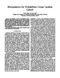
Figure 2.1: Barendregt's -Cube

! 2 ! P P! ! P2 P!

(F ;) (F ;) (F 2;) (F ;) (F ;2) (F ;) (F 2;) (F ;2) (F ;) (F 2;2 ) (F ;) (F 2;) (F 2;2 ) (F ;) (F ;2) (F 2;2 ) (F ;) (F 2;) (F ;2) (F 2;2 ); where the pair (s1; s2 ), in the rule (F s1 ;s2 ), denotes the sort of the premise and of the conclusion, respectively; as example, the rule (F 2; ) denotes the following rule: ?; a:A `t B : 2 (F 2;) ? `t a:A:B : which corresponds to the introduction of a polymorphic-type. Figure 2.1 shows the eight typed systems arranged as vertices of the Barendregt's cube . Observe that, in this cube, the edges are intended as an inclusion relation between systems.


25

De nition 2.1.9 i) If ? `t A : , then A is a \type" in the context ?. ii) If ? `t A : 2, then A is a \kind" in the context ?. iii) If ? `t A : B and ? `t B : , then A is a (typed) -term in the context ?. iv) If ? `t A : B and ? `t B : 2, then A is a \constructor". Since `t : 2, it follows that a type is also a constructor.

In what follows, we adopt the notational convention on the names of pseudo-terms: -term-variables will be denoted by x, y, z, :: :, and -terms by M , N , : ::, whereas typeand constructors-variables will be denoted by , , , : : :, and types and constructors by , , , , : :: This choice will be useful in the next chapter, when those conventions will be taken as part of the syntax of a new \strati ed" presentation of the -cube. Remark 2.1.10 Most of the systems in the -cube appear elsewhere in the literature. In particular: the system ! corresponds to Church's typed system [Chu41], whereas 2 is the second order polymorphic -calculus, which is essentially Girard's system F [Gir86]. The step to go from system ! to system 2 is to allow for polymorphic-types, i.e., introducing the mechanism of binding (free) constructor-variables, as for

? `t ::M : ::, and replacing them by constructors, as in ? `t M : [ =]. The step to go from system ! to system ! is to allow for higher-order types, i.e., types dependent on types , that makes it possible to derive ? `t (:: ) : . The step to go from system ! to system P, is to allow for the construction of dependent-types, i.e., types dependent on -terms, that makes it possible to derive ? `t (x:: )N : .


26

So, in the previous table, the rule (F 2;) introduces polymorphic-types, the rules (F ;2), and (F 2;2 ) introduces the higher-order types, and dependent-types respectively. The well known systems of the simply typed -calculus, and the system F of Girard are given in an equivalent constructive version. The system P is often called Logical Framework [HHP92]. The system P! (also called CC) is the Calculus of Construction of Coquand and Huet [CH88].

2.1.1 Properties of Barendregt -Cube

The properties of this cube are proved in [Bar92, GN91]. We list just a few of them, those that are used in the next chapters. Proposition 2.1.11 If ? `t A : s1 and ? `t A : s2, then s1 s2 .

Property 2.1.12 A[B=b][C=c] A[C=c][B [C=c]=b], provided b 62 FV (C ). Property 2.1.13 (Church-Rosser Property for Typed Systems) A = B & ? `t A : C & ? `t B : C ) 9 D [A ! ! D & B !! D]. Property 2.1.14 The General Typed System derives judgments of the following shapes:

? `t M : , ? `t : K , or ? `t K : 2. De nition 2.1.15 i) A typed legal context is inductively de ned as follows: a) " is legal; b) ?; a:A is legal ( ) ? is legal & ? `t A : s, & a 62 Dom (?). ii) The relation v is inductively de ned on legal contexts as follows: a) " v ?; b) ? v ?0 ) ?; a:A v ?0; a:A; c) ? v ?0 ) ? v ?0;a:A.

Property 2.1.16 i) ? v ?0 & ? ` A : B ) ?0 ` A : B. ii) D: ?; c:C `t A : B ) 9 D0 D [D 0: ? `t C : s]. Property 2.1.17 (Typed Generation Lemma) i) ? `t a : A ) 9 s, B [? `t B : s & a:B 2 ? & A = B].

2.2. Constructive Type Systems

27

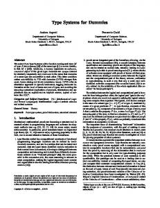
Syntax of Type!: ::= j !

x: 2 ? 2 Type! (Axiom ) ? `t x: (!Elim)

? `t M : ! ? `t N : ? `t MN :

(!Intro)

?; x: `t M : ? `t x::M : !

Figure 2.2: Church's Typed -Calculus ii) ? `t a:A:B : C ) 9 s1 , s2 , s3 [? `t A : s1 & ?; a:A `t B : s2 & C = s3]. iii) ? `t a:A:B : C ) 9 s, D [? `t a:A:D : s & ?; a:A `t B : D & C = a:A:D]. iv) ? `t AB : C ) 9 D, E [? `t A : d:D:E & ? `t B : D & C = E [B=d]]. Property 2.1.18 ? `t A : B ) B 2 _ ?t `t B : s. In particular, if A M , then B , and is a type with respect to the context ?. Property 2.1.19 (Termination for typed terms) If ? `t A : B , then A and B are both strongly normalizing.

The next section will present the main dierences between the systems in the cube and their original versions. Moreover, Section 2.3 will present the main ideas underlying dependent-types of P.

2.2 Constructive Type Systems In this section, we show the dierences between the original presentation of the simply and polymorphic typed -calculi, presented in Figures 2.1.1 and 2.1.1 , and their presentations in the -cube. In this cube, the systems are given in a constructive way, in the sense that types are formally generated by the system itself and not in the informal metalanguage. There is a constant such that : corresponds to 2 Type. So, the original notion of context as set containing at least all the declarations for the free variables of the subject of the judgment, becomes the notion of context as list , containing


28

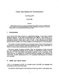
Syntax of Type8: ::= j ! j 8:

x: 2 ? 2 Type8 (Axiom ) ? `t x: (!Elim)

? `t M : ! ? `t N : ? `t MN :

? `t M : 8: 2 Type8 (8Elim) ? `t M : [ =]

(!Intro)

?; x: `t M : ? `t x::M : !

(8Intro)

? `t M : 62 FV (?) ? `t :M : 8:

Figure 2.3: The Girard's Polymorphic -Calculus at least all the declarations for the free variables of both the subject and the predicate of the judgment. We will now show, with help of an example, how some informal statements can be formally written as derivations in the -cube. i) Consider the following de nition of arrow-type formation: ; 2 Type ) ! 2 Type. This corresponds to the following derivation in the -cube: (Axiom ) ... (Proj ) " `t : 2 (1) ... (Weak ) : `t : : `t : 2 (2) (Weak ) :; : `t : :; : `t : (3) :; :; x: `t : (I ) :; : `t x:: : where (1); (2), and (3) stand for 62 Dom ("), 62 Dom (:), and y 62 Dom (:; :) respectively, and we will see in this section that x:: ! , if x 62 FV () [ FV ( ). ii) Consider the following derivation in the original presentation of the simply typed -calculus of Church:

Example 2.2.1

2.3. Type Dependencies

29

! 2 Type y:! `Ch y : ! This derivation will be denoted in its constructive version !, by the following derivation: D y 62 Dom (:; :) (Proj ) :; :;y:x:: `t y : x:: where D is the derivation of part (i), and x does not occurs in , and . (Axiom )

Remark 2.2.2 Observe that the order of the type-variables in the context of the rst example is not important, although in the second example it is. In fact, we can derive (using dierent derivations)

:;: `t x:: : ; :; :; y:x:: `t y : x:: ; but we cannot derive

:; y:x:: ; : `t y : x:: ; :; y:x:: ; : `t y : x:: ; y:x:: ;:; : `t y : x:: ; as one easily checks by looking at the rule schemes of the cube. So, modifying the order of a (legal) context aects derivability.

2.3 Type Dependencies In the previous section, we showed the main dierences between the original presentation of the simply typed -calculus of Church, system F , and their equivalent variants in the Barendregt's cube. In this section, we present the main ideas that motivate the use of dependent-types. Dependent-types have been fruitfully used for fully formalizing mathematical objects (see AUTOMATH [dB80], LF [HHP92], and NUPRL [Con86], and the Type Theory of Martin-Lof [Mar84]). What follows is mainly taken from [Bar92]. Dependent-types where invented by N.G. de Bruijn in the seventies; the main idea is the introduction of product-types . Product-types have the following form:

30

Chapter 2. Typed Systems for the -Calculus x:: ,

where x is a -term variable, and are types, and x may occur free in . The underlying idea is as follows: for every x of type , there exists a term M [x] of type [x], where M [x] and [x] denote that M and contain free occurrences of x. Then we can build the function:

x::M [x] of type x:: [x]. So, by interpreting types as set and -abstractions as functions over sets, we get a function from the domain, represented by the interpretation of , to the codomain, represented by the interpretation of a family of types, each one depending on the input argument of the above function. If the bound variable x does not occur in , i.e. (with a little abuse of notation), [ ] , then the family of sets obviously collapses in a single set, representing the codomain of the function. In this case we recover the usual interpretation of the arrow-type. The typed systems with dependences where invented to prove the validity of a logic formulas in the predicate calculus PRED. In fact, the main idea is as follows: [dB80] Given a logic formula ' in PRED, there exist a translation map jj jj from formulas in PRED into types in P such that ' is a valid formula if and only jj'jj is inhabited in P, i.e. there exists ?, and M , such that ? `t M : jj'jj is derivable in system P. In fact, system P is given that name because of PRED. The rst project realizing this correspondence was AUTOMATH [dB80], which uses a slight modi cation of P. The main dierence between P and the system used by AUTOMATH, is that in P the kind of a logic formulas is , whereas AUTOMATH introduces a special constant Prop of kind , which represents the kind of well formed formulas, and a logic formula ' is valid if and only if its translation, T j'j is inhabited, where T is a special variable of kind Prop!. A recent system using dependent-types for formalizing logics is the system LF [HHP92], developed at the Edimburgh University by Harper, Honsell and Plotkin. It is essentially the system P.

2.4. The Strati ed Presentation of the TS Cube

31

2.4 The Strati ed Presentation of the TS Cube In the previous section, we showed the original presentation of the Barendregt's cube of typed systems, as in [Bar92]. In this section, we present a `strati ed` version of the systems in the cube, i.e., we will split the terms considered by Barendregt in three dierent classes, being those of -terms, constructors, and kinds, such that each class comes with its own derivations rules. This should enable the appreciation of the presentation of our cube of type assignment systems in the next chapter. Notational Conventions In this section (and in Chapters 2, and 3), a term will be either an (un)typed -term , a constructor, a kind, or a sort. The symbols M , N , P , Q, : : : range over (un)typed -terms; , , , , : : : range over constructors; K ranges over kinds; s ranges over sorts: A, B , C , D, : : : range over arbitrary terms; x, y, z, : : : range over -term-variables; , , , : : : range over constructor-variables; a, b, c, : : : range over -term-variables and constructor-variables. The symbol ? will range over contexts. All symbols can appear indexed. The symbol denotes the syntactic identity of terms, and we will consider terms modulo -conversion. The notation ni=1ai:Ai:B is an abbreviation of a1:A1: an:An :B . De nition 2.4.1 (Abstract Strati ed Typed Syntax) Given the set of sorts, i.e.:

s 2 f; 2g, the sets of typed -terms (t), typed constructors (Const ), and typed kinds (Kindt ) are mutually de ned by the following grammar, where M; , and K are metavariables for -terms, constructors and kinds respectively:

M ::= x j x::M j MM j :K:M j M ::= j x:: j :K: j x:: j :K: j j M K ::= j x::K j :K:K The set Tt of typed terms is the union of the sets t , Const and Kindt .

32


Remark 2.4.2 The introduction of three classes of `terms' in De nition 2.4.1 induces a strati ed version of the set derivation rules; each class comes with its own derivations rules. The names of the rules are, to save space, restricted to a few characters. We have tried to use an orthogonal approach in baptizing the rules: in general, a name for a rule is composed like (X ?YZ ), meaning that: i) it is a rule that follows the syntax of objects in class X , where X is omitted for -terms, is C for constructors, and K for kinds, ii) Y is either a) I for an introduction rule, that are used to deal with the various -abstractions, b) E for an elimination rule, that deal with applications, c) F for a formation rule, that deal with the -abstraction, iii) and Z is used (as X above) to indicate the class either of the bound variable (in case of an introduction or formation rule), or of the right-hand side term in an application (in case of a formation rule). De nition 2.4.3 (General Typed System) i) The General Typed System proves judgments of the form ? `t A : B , where ? is a context and A : B is a statement. ii) The General Typed System's set of rules, can be divided in four groups, depending of the subjects of the statements: Common Rules ? `t A : s a 62 Dom (?) ? `t A : B ? `t C : s c 62 Dom (?) (Proj) ( Weak ) ?; a:A `t a : A ?; c:C `t A : B (Conv ) ? `t A : B ? `t C : s B = C ? `t A : C Typed -Term Rules ?; x: `t M : ? `t M : x:: ? `t N : (E ) (I ) ? `t x::M : x:: ? `t MN : [N=x] ?; :K `t M : ? `t M : :K: ? `t : K (IK ) (EK ) ? `t :K:M : :K: ? `t M : [ =]

2.4. The Strati ed Presentation of the TS Cube Typed Constructor Rules ?; x: `t : K (C -IC ) ? `t x:: : x::K ?; :K1 `t : K2 (C -IK ) ? `t :K1: : :K1:K2 ?; x: `t : (C -FC ) ? `t x:: : Typed Kind Rules

(Axiom)

" `t : 2 ?; :K1 `t K2 : 2 ? `t :K1:K2 : 2

33

? `t : x::K ? `t M : ? `t M : K [M=x] ? `t : :K1:K2 ? `t : K1 (C -EK ) ? `t : K2[ =] ?; :K `t : (C -FK ) ? `t :K: :

(C -EC )

(K -FC )

?; x: `t K : 2 ? `t x::K : 2

(K -FK ) iii) Let the following sets of rules be de ned by: Base-Rules = f(Axiom ); (Proj ); (Weak ); (I ); (E ); (C -FC )g, Polymorphism = f(IK ); (EK ); (C -FK )g, Dependencies = f(C -IC ); (C -EC ); (K -FC ); (Conv )g, Higher-Order = f(C -IK ); (C -EK ); (K -FK ); (Conv )g. When allowing abstraction to constructor-variables, redexes in constructors can be created. The rule (Conv ) is present in both the sets Higher-Order and Dependencies because we want to identify -equivalent constructors. iv) The eight typed systems in the strati ed version of Barendregt's cube can be represented by the set of derivation rules used in each system.

! ! 2 ! P P! P2 P!

= = = = = = = =

Base ?Rules ; ! [ Higher ?Order ; ! [ Polymorphism ; ! [ Higher ?Order [ Polymorphism ; ! [ Dependencies ; ! [ Dependencies [ Higher ?Order ; ! [ Dependencies [ Polymorphism ; ! [ Dependencies [ Higher ?Order [ Polymorphism :

34


For each set of rules S , we write ? `S A : B to indicate that ? `t A : B can be derived using only the rules in S . The expression `system S ' refers to the typed system obtained by restricting the full system to allow only the rules in S . If ? `t M : for a typed -term M , then ? `t : (see [Bar92]). In this case we say that is a type or, to be more precise, a type with respect to the context ?. De nition 2.4.4 i) We write D: ? `t A : B to express that D is a derivation for the judgment ? `t A : B. ii) We write D 0 D when D 0 is a subderivation of D. iii) In what follows we will use the notation:

C1 : : : D: C

Cn

(R)

to denote the derivation D, proving the judgment C , that is obtained by applying the rule (R) to the premises C1 ; :: : ; Cn , which are conclusions of some derivations.

Chapter 3 The Cube of Type Assignments Systems TAS Introduction In the previous chapter, we saw that terms of the -calculus can be directly decorated with types. In this fully typed approach, every closed term comes directly with a unique, intrinsic type. In this chapter, we discuss another way of giving types to terms of the -calculus: the type assignment approach. It was introduced by Curry [Cur34] for the Theory of Combinators, and then modi ed by Curry [CF58, CHS72] for the -calculus; it, essentially, proves judgments of the shape: ? ` M : , where M is a term of the (untyped) -calculus, is a type (i.e. an element of a given set Type of types), and ? is a context, assigning types to the free variables of M and . Such a judgment means that we can assign the type to the -term M , when types are assigned to the free variables of M and as speci ed in the context ?. In this approach, types are viewed as predicates, or properties, of terms, and each closed term can be assigned either none or in nitely many types. This approach were called a la Curry by Barendregt, and these systems are sometimes called type assignment systems. When we look at -calculus as a paradigmatic programming language, this approach corresponds to ML-like languages, where the user can write programs in a completely 35

36

Chapter 3. The Cube of Type Assignments Systems TAS

untyped language, and types are automatically inferred at compile time. The approach can be also intended as the construction of an abstract interpretation of the program, that can be used as a correctness criterion. In [Cur34, Lei83, GR88], it was observed that some of the type assignment systems already known in the literature can also be obtained from a typed system through an erasing function that erases type information from terms in a typed system. In particular, the Curry type assignment system [Cur34] (F1) can, in this way, be obtained from !, the polymorphic type assignment system (F2) [Lei83] from 2, and the higherorder type assignment system (F!) [GR88] from the higher-order -calculus !. For those systems, if D is a typed derivation, and E is the above meant erasing function, then by applying E to the \subject" of every judgment in D, we obtain a valid type assignment derivation with the same structure of the typed one. Vice versa, every type assignment derivation can be viewed as the result of an application of E to a typed one. In particular, the erasing function E induces an isomorphism between every typed system on the dependency-free side of Barendregt's cube and the corresponding type assignment system. In [GHR93], the erasing function was extended in a natural way to all typed systems in Barendregt's cube, including the systems with dependent-types, as studied in [Ber88, HHP92]. The essential dierence is that the domain of E was extended to includes types too, since now terms can occur in types. To be precise, if a typed system consists of a set S of derivation rules, the rules of the corresponding type assignment system can be obtained by applying E to every object occurring in the rules of S . This erasing function E induces a cube of type assignment systems. Namely, for every typed system St in Barendregt's cube, there is a corresponding type assignment system Su , of which the rules are obtained from those of St via the extended erasing function E . Note that, in this setting, if ? ` M : is a typed judgment, then the corresponding type assignment judgment is E (?) ` E (M ) : E (), where now E () can be dierent from (E (?) from ?), in case is a dependent-type (? contains dependent-types). The fact that in [GHR93] also systems that contain dependences were considered, was a rst attempt to study dependent-types in a type assignment approach. In that paper, and also in [PM89], was proved that the introduction of dependences does not increase the expressiveness of a system, i.e., the terms typable in a type assignment system with dependences are all nothing but those typable in the similar system, obtained

37 from the rst by erasing the dependences. The above mentioned erasing function E , at least for the dependency-free plane of TS and TAS , induces an isomorphism between derivations in corresponding systems. More precisely, if D is a derivation in a typed system, by applying E to every object (i.e. term, constructor, or kind) in D, a valid derivation in the corresponding type assignment system is obtained. Vice-versa, again only for dependency-free systems, every type assignment derivation can be obtained by applying E to a typed one. The `formulae-as-types' principle [How80] can be extended to the above type assignment systems as follows: Given an untyped term M , if we can assign a type in the type assignment systems F1(respectively F2, and F! ), with a derivation D, then: i) D can be interpreted as the coding of a proof for the logic formulas ' which corresponds to the interpretation of the type assigned to M . ii) M can be interpreted as the coding of a \logical proof schema", whose instances (of the schema) prove, respectively, all the logic formulas 'i's that can be interpreted as the types i's that can be assigned to M .

Clearly, the fact that the classes of derivations for typed and a type assignment systems are isomorphic means that they have the same underlying logical system. In this chapter, we show an example of a inhabited type in TAS , that cannot be obtained through erasure of an inhabited type in TS . This negative result of course implies that the logical sides of these two cubes are dierent; however, this dierence only shows up in the plane of the cube with dependences, where already TS has lost a clear connection with logic [Ber88]. Furthermore, it is also our opinion that there is more to types than just logic: studying types is not solely justi able through the connection between types and logic, as is clearly shown by, for example, the type system developed for ML that models typeconstants and recursion [Mil78], and the intersection-type discipline [BCD83]. In our view, the main motivation for TAS comes from the ML-style of approaching types: to have type-free code with type assignment seen as a correctness criterion, or safety means, but always outside of programs rather than built in. Certainly, in order to be correctly applied in this way, a type assignment system must enjoy some fundamental properties,

38


like the Church-Rosser property, the subject-reduction property and normalization. We prove these properties for all systems in TAS . So, TAS can make sense even if it does not t the corresponding TS : it is just another way to select legitimate code. Studying type systems with dependences can be of value from the point of view of abstract interpretation; such type assignment system could introduce a more re ned notion of types in a programming language setting. For example, since the version of F1 with dependences is decidable, and the core of the type system for ML is based on F1, designing a version of ML with dependent-types seems feasible. This chapter is organized as follows: Section 3.1 contains the strati ed presentation of the cube of type assignment systems. Starting from the typed strati ed cube, we will de ne an erasing function E and, using this function, obtain the related cube of type assignment systems. The same approach can be found in [GHR93]. In Section 3.2, the properties of the type assignment systems belonging to this cube are studied; Sections 3.3 , and 3.4 contain the proofs of the Church-Rosser property, and of the subject reduction, and nally Section 3.5 contains the proof of strong normalization.

3.1 The Cube of Type Assignment Systems In this section, we will present the cube of type assignment system as was rst presented in [GHR93]. The de nition of the type assignment cube is based on the de nition of the type-erasing function E , to be de ned below, that erases all type information in typed -terms. In fact, both the syntax of terms, and the rules of the type assignment systems in the cube are obtained directly from the corresponding syntax and rules of the typed systems in Barendregt's cube, by applying E . Note that, since both constructors and kinds can depend on -terms, E can modify all objects. Since -terms do not contain type information, we cannot create -terms dependent on types. From now on, we will reserve the name typed systems (TS ) for the systems of Barendregt's cube, and we reserve the expression type assignment systems (TAS ) for the systems to be de ned below. As already mentioned in the introduction, for the plane of the TS -cube without dependences there exists a function that, erasing type information from typed -terms, allows to switch from a typed system to a corresponding type assignment system. To be

3.1. The Cube of Type Assignment Systems

39

precise, it erases type information from -bindings occurring in -terms, while leaving all type information that decorates bindings in constructors and kinds intact. In [GHR93], a more general function E was de ned, by extending the domain of the above function to terms with dependences in a natural way, as shown in the De nition 3.1.1. De nition 3.1.1 i) f; 2g is the set of sorts . ii) The sets of -terms (), constructors (Cons), and kinds (Kind) are mutually de ned by the following grammar, where M; and K , are metavariables for -terms, constructors and kinds respectively: M ::= x j x:M j MM ::= j x:: j :K: j x:: j :K: j j M K ::= j x::K j :K:K The set Tu of terms is the union of the sets , Cons and Kind.

The elimination of type information from a typed -term yields an untyped -term. Both the syntax and the rules of the TAS cube can be obtained directly from the corresponding rules of the TS cube by applying the following type-erasing function E . De nition 3.1.2 The erasing function E : Tt ! Tu is inductively de ned as follows: i) On t.

E (x) = x; E (MN ) = E (M )E (N ); E (M) = E (M ); E (x::M ) = x:E (M ); E (:K:M ) = E (M ):

40


ii) On Const .

E () = ;

E (x:: ) E (:K: ) E (x:: ) E (:K: ) E ( ) E (M )

= = = = = =

x:E ():E ( ); :E (K ):E ( ); x:E ():E ( ); :E (K ):E ( ); E ()E ( ); E ()E (M ):

iii) On Kindt .

E () = ;

E (x::K ) = x:E ():E (K ); E (:K1:K2) = :E (K1):E (K2): The erasing function is extended to contexts in the obvious way and we use the notation E (?). Note that the behaviour of E is such that, in the image of E , -terms are completely untyped, while constructors and kinds are `partially' typed. The notions of free variables, subterms and -reduction are similar to their `fully typed' counterparts, but slightly modi ed, according to the untyped term syntax. De nition 3.1.3 i) The set of free variables of A is de ned as in De nition 2.1.2, extended with: FV (x:M ) = FV (M ) n fxg. ii) Substitution for -terms is de ned as in De nition 2.1.3, extended with: (x:M )# x:M #. iii) The set of subterms of A is de ned as in De nition 2.1.5, extended with: ST (x:M ) = fx:M g [ ST (M ).

The ùntyped variant' of Property 2.1.12 also holds.


41

Lemma 3.1.4 A[B=b][C=c] A[C=c][B [C=c]=b], provided b 62 FV (C ). Proof: By induction on the de nition of substitution. [A a and a 6 b and a 6 c]: then a[B=b][C=c] a a[C=c][B [C=c]=b]. [A b]: then b[B=b][C=c] B[C=c] b[B [C=c]=b] b[C=c][B[C=c]=b]. [A c]: then c[B=b][C=c] C c[C=c][B [C=c]=b]. [A A1A2]: then (A1A2)[B=b][C=c] A1[B=b][C=c]A2[B=b][C=c] (IH ) A1[C=c][B [C=c]=b]A2[C=c][B [C=c]=b] (A1A2)[C=c][B [C=c]=b]. [A a:A1:A2]: then (a:A1:A2)[B=b][C=c] a:A1[B=b][C=c]:A2[B=b][C=c] (IH ) a:A1[C=c][B[C=c]=b]:A2[C=c][B [C=c]=b] (a:A1:A2)[C=c][B [C=c]=b]. [A x:M ]: then (x:M )[B=b][C=c] x:M [B=b][C=c] (IH )x:M [C=c][B [C=c]=b] (a:A1)[C=c][B[C=c]=b]. [A a:A1:A2]: then (a:A1:A2)[B=b][C=c] a:A1[B=b][C=c]:A2[B=b][C=c] (IH ) a:A1[C=c] [B [C=c]=b]:A2[C=c][B[C=c]=b] (a:A1:A2)[C=c][B[C=c]=b]. De nition 3.1.5 ( -reduction, -conversion)

i) Let:

(x:: )M ! [M=x]; (:K:) ! [ =]; (x:M )N ! M [N=x]: The -reduction ! is de ned as the contextual closure of these rules, i.e.:

A! A0 A! A0 M ! M 0 A! A0 A! A0 A! A0 A! A0

) ) ) ) ) ) )

AB ! A0B BA! BA0 x:M ! x:M 0 a:A:B! a:A0:B b:B:A! b:B:A0 a:A:B! a:A0:B b:B:A! b:B:A0:

ii) -reduction ! ! is the re exive, transitive closure of ! , i.e.:


42

A! ! A0 &

A! A0 A0 ! ! A00

A! ! A ) A !! A0 ) A !! A00

iii) -conversion = is the minimal equivalence relation generated by ! ! , i.e.:

A! ! A0 ) A = A0 A = A0 ) A0 = A A = A0 & A0 = A00 ) A = A00 In the next lemma, we show that -conversion and substitution behave well together. Lemma 3.1.6 If A = B , then A[C=c] = B[C=c]. Proof: By induction on the de nition of = . We just consider the case when A is a redex, by induction on ! ! ; the complete proof follows easily by induction. [A x:M and B M [N=x]]: then ((x:M )N )[C=c] (x:M )[C=c]N [C=c] (x:M [C=c])N [C=c] ! M [C=c][N [C=c]=x] which is equal, by Lemma 3.1.4 , to M [N=x][C=c]. [A (x:: )M and B [M=x]]: then ((x:: )M )[C=c] (x:: )[C=c]M [C=c] (x:[C=c]: [C=c])M [C=c] ! [C=c][M [C=c]=x] which is equal, by Lemma 3.1.4, to [M=x][C=c]. [A (:K:) and B [ =]]: then ((:K:) )[C=c] (:K:)[C=c] [C=c] (:K [C=c]:[C=c]) [C=c] ! [C=c][ [C=c]=] which is equal, by Lemma 3.1.4 , to [ =][C=c].

The notion of statement and context are de ned as in De nition 2.1.6, and 2.1.7, taking into account the dierences in syntax. Given the dierence in syntax, the type assignment judgments and rules as presented in De nition 3.1.7 are only in appearance similar to those of De nition 2.4.3 . Note that the denotation of a rule is only dierent for the rules (I ), (IK ) and (EK ). We will, therefore, take the liberty of using the same notation and names for rules.


43

De nition 3.1.7 (General Type Assignment System ) i) The following rules are used to derive judgments of the form ? ` A : B, where ? is a context and A : B is a statement. ii) The General Type Assignment System set of rules, can be divided in four groups, depending of the subjects of the statements: Common Rules ? ` A : s a 62 Dom (?) (Proj) (Conv ) ? ` A : B ? ` C : s B = C ?;a:A ` a : A ? ` A:C ? ` A : B ? ` C : s c 62 Dom (?) (Weak) ?; c:C ` A : B -Term Rules ?; x: ` M : ? ` M : x:: ? ` N : (I ) (E ) ? ` x:M : x:: ? ` MN : [N=x] ?; :K ` M : ? ` M : :K: ? ` : K (EK ) (IK ) ? ` M : :K: ? ` M : [ =] Constructor Rules ?; x: ` : K ? ` : x::K ? ` M : (C -IC ) ( C E ) C ? ` x:: : x::K ? ` M : K [M=x] ?; :K1 ` : K2 ? ` : :K1:K2 ? ` : K1 (C -IK ) ( C E ) K ? ` :K1: : :K1:K2 ? ` : K2[ =] ?; x: ` : ?; :K ` : (C -FC ) (C -FK ) ? ` x:: : ? ` :K: : Kind Rules ?; x: ` K : 2 ( K F ) (Axiom) C " ` :2 ? ` x::K : 2 ?; :K1 ` K2 : 2 (K -FK ) ? ` :K1:K2 : 2 iii) Let the following sets of rules be de ned as in De nition 2.4.3 (iii), i.e.: Base-Rules = f(Axiom ); (Proj ); (Weak ); (I ); (E ); (C -FC )g, Polymorphism = f(IK ); (EK ); (C -FK )g, Dependencies = f(C -IC ); (C -EC ); (K -FC ); (Conv )g, Higher-Order = f(C -IK ); (C -EK ); (K -FK ); (Conv )g.


44

Notice that, unlike for the derivation rules of De nition 2.4.3 (ii), the subject does not change in the type assignment rules (IK ) and (EK ). These two, together with the rules (Weak) and (Conv), are called the not syntax-directed rules . iv) The eight type assignment systems can be distinguished, as in De nition 2.4.3 (iv), by the set of derivation rules used in each system. F1 F! F2 F! DF1 DF! DF2 DF!

= = = = = = = =

Base?Rules ; F1 [ Higher ?Order ; F1 [ Polymorphism ; F1 [ Higher ?Order [ Polymorphism ; F1 [ Dependencies ; F1 [ Dependencies [ Higher ?Order ; F1 [ Dependencies [ Polymorphism ; F1 [ Dependencies [ Higher ?Order [ Polymorphism :

Like for TS we will write, for each set of rules S , ? `S A : B to indicate that ? ` A : B can be derived using only the rules in S . Then, Figure 3.1 shows the eight type assignment systems arranged as vertices of a cube (the TAS cube). Also in this cube the edges are intended as an inclusion relation between systems. The notion of derivation and subderivation for a judgment are the same as in De nition 2.4.4 , and an analogue of Property 2.1.14 also holds: Lemma 3.1.8 The General Type Assignment System derives judgments of the following shapes:

? ` M : , ? ` : K , or ? ` K : 2. Proof: By looking at the rules and by observing that the sets Cons, and Kind are closed for the substitution of -term-variables by terms, and constructor-variables by constructors. As before, a type is a constructor of kind (and this is again a context-dependent property). A -term M is typable if there are a context ? and a constructor , such that ? ` M : (we will prove in Section 3.2 that must be a type).


F2

>

45

F!

-

6 -

6

F1

DF !

>

6

DF 2 6

>

F!

-

-

DF 1

DF !

>

Figure 3.1: The Cube of the Type Assignment Systems Remark 3.1.9 Notice that, in the left-hand side of the cube, the constructors coincide with the typed ones, because there they cannot depend on -terms. This no longer holds in the right-hand side: here we can build constructors like

(x:: )N , where N is a pure, untyped -term. The system F1 corresponds to the well-known Curry type assignment system, whereas F2 is the type assignment version of the second order -calculus. The three dimensions in this cube of type assignment systems correspond, as for Barendregt's cube, to the introduction of polymorphic-types , higher-order types and dependent-types. The systems DF 1, DF!, DF2, and DF ! represent the rst attempt to de ne type assignment systems with dependent-types .

46


3.2 Basic Properties of TAS In this section, we will prove that all systems in the TAS cube satisfy good computational properties, like the Church-Rosser property, the subject reduction property, and strong normalization of typable terms. To prove these results, we need more de nitions and technical lemmas, stating properties of the systems that are also of independent interest. The following proposition states that every term, typable by or 2, cannot be typable by both, and guarantees consistency of the system. This property holds for the, so called, functional pure type systems [Bar91]. Proposition 3.2.1 If ? ` A : s1 and ? ` A : s2 , then s1 s2. Proof: This is an obvious consequence of Lemma 3.1.8. De nition 3.2.2 A legal context is inductively de ned as follows: i) The empty context " is legal; ii) ?; a:A is legal if and only if ? is legal, ? ` A : s, and a 62 Dom (?).

In the next lemma, we show that every context in a derivable judgment is also legal. Lemma 3.2.3 If ? ` A : B , then ? is legal. Proof: By induction on derivations. [(Proj), (Weak )]: let ?= ?0; c:C , for some ?0; c, and C . Then the conclusion is ?0; c:C ` A : B. From the assumptions we get ?0 ` A : B , and ?0 ` C : s, and c 62 Dom (?0). By induction ?0 is legal, and hence, by De nition 3.2.2 , ?0; c:C is legal. [(Conv ), (Elimination rules)]: by induction. [(Introduction, Product rules)]: then the conclusion is either ? ` c:C:D : c:C:E , or ? ` x:M : c:C:E , or ? ` c:C:D : s, for some x; c; C; D; E; M , and s. Take, as example, the rst case: from the assumption we get ?; c:C ` D : E .

3.2. Basic Properties of TAS

47

Then, by induction ?; c:C is legal, and, by De nition 3.2.2 , ? is legal. We de ne the following relations on legal contexts: De nition 3.2.4 i) ? v ?0 if and only if ? is a pre x of ?0. ii) The relation v is inductively de ned as a) " v ?; b) If ? v ?0, then ?; a:A v ?0 ; a:A; c) If ? v ?0, then ? v ?0; a:A.

For these relations, the following lemma holds.

Lemma 3.2.5 i) If ?1 v ?2 , then ?1 v ?2 . ii) If ?1 v ?2 then Dom (?1 )Dom (?2). iii) If ?1 ; a:A; ?2 v ?3; a:A then ?2 = ". iv) If ?1 ; a:A; ?2 v ?3; a:A; ?4 then ?1 v ?3 , and Dom (?2 ) Dom (?4 ).

Proof: Easy, using De nition 3.2.4 (ii) .

The next lemma states that all statements of a context occurring in a judgment are obtained by proper subderivations. Lemma 3.2.6 If D : ?; c:C ` A : B , then D 0 : ? ` C : s, and D0 D. Proof: By easy induction on derivations.

The next lemma states that the free variables a derivable the statement are declared in the context of the judgment, and that if a statement is derivable, then it is also derivable in a bigger context.

Lemma 3.2.7 If ? v ?0 and ? ` A : B , then i) (Free Variable) FV (A) [ FV (B ) Dom (?). ii) (Thinning) ?0 ` A : B . Proof: i) By induction on derivations.

48


[(Weak ), (Proj )]: by induction. [(Introduction, Product rules)]: take for instance the (C -IK ) rule: D : ?; :K1 ` : K2 (C -I ) K ? ` :K1: : :K1:K2: By induction, FV ( ) [ FV (K2) Dom (?; :K1) = Dom (?) [ fg. By Lemma 3.2.6, we nd D0 D such that D0 : ? ` K1 : s, so, by induction, FV (K1) Dom (?). Since: FV (:K1: ) [ FV (:K1:K2) = FV (K1) [ (FV ( ) [ FV (K2)) n fg, the thesis follows. [(Elimination rules), (Conv )]: take for instance the (E ) rule: ? ` M : x:: ? ` N : (E ) ? ` MN : [N=x]: By induction, if c 2 FV (M ) [ FV (x:: ), then c 2 Dom (?), and if c 2 FV (N ) [ FV (), then c 2 Dom (?). Observe that: FV ( [N=x]) = FV ( ) n fxg [ FV (N ), and the thesis follows. ii) By induction on derivations. [(Proj),(Weak)]: take for instance the (Proj) rule: ?1 ` B : s b 62 Dom (?1) (Proj ) ?1; b:B ` b : B; for some ?1. Then, by Lemma 3.2.5 (ii), Dom (?1; b:B ) Dom (?0), i.e., ?0= ?01; b:B;?02, for suitable ?01, ?02. By Lemma 3.2.5 (iv), ?1 v ?01, and, by induction, ?01 ` B : s. Since ?0 is legal, also b 62 Dom (?01). Apply a (Proj ) rule to obtain ?01; b:B ` b : B . Again by the legality of ?0, it follows that for all c:C 2 ?02, there exists ?002 v ?02, such that ?01; b:B;?002 ` C : s. So, we can apply a (Weak ) rule a suitable number of times, to get ?1; b:B;?02 ` b : B , as desired. [(Introduction, Product rules)]: take for instance the (C -IC ) rule:


49

?; x: ` : K (C -IC ) ? ` x:: : x::K:

By induction, for every ?0, such that ?; x: v ?0, we have ?0 ` : K . By Lemma 3.2.5 (ii), we have that ?0 = ?01; x:; ?02, for suitable ?01, and ?02. By Lemma 3.2.5 (iv), ? v ?01, so ? v ?01,x:. By induction, ?01;x: ` : K . Apply a (C -IC ) rule to obtain ?01 ` x:: : x::K . By the legality of ?0 (using the same reasoning as in the (Proj ) case), apply a (Weak) rule a suitable number of times. [(Elimination rules), (Conv )]: by induction.

The following relation is introduced to abbreviate a sequence of derivation rules (IK ) and (EK ), that together correspond to polymorphism, and also takes the presence of rule (Conv ) into account. It will be of use in Lemma 3.2.9 and in Theorem 3.4.4. De nition 3.2.8 We de ne the relation on constructors inductively by:

) :K: ) =

; :K:; [=]; :

The four cases in De nition 3.2.8 re ect, respectively, an application of rule (Conv), (IK ), or (EK ), and a sequence of not syntax-directed rules. Worth noticing is the second case of De nition 3.2.8, because it illustrates an important dierence between the original presentation of the polymorphic type assignment system [Lei83], and our presentation as a system in the topology of the TAS cube. The equivalent rule for (IK ) in the polymorphic type assignment system is: ? ` M : 62 FV (?) (8?Intro) ? ` :M : 8: The type 8: is essentially the constructor ::, and 62 FV (?) is a side-condition, indicating that binding of the type-variable is only allowed when does not occur free


50

in any predicate belonging to the context. The polymorphic type assignment system needs this side-condition to avoid to assign, for example,

x: ` x : 8:. The TAS presentation of this system does not require this extra condition on the derivation rule (IK ): in fact, types are generated by the system itself, using only legal contexts, which are essentially linear ordered sets of declarations, in the derivations. In these systems, it is impossible to apply a (IK ) rule to the derivation for

:; x: ` x : , because : is not the right-most declaration in the context; when ?; : ` M : , then, by legality of the context, does not occur in ?, so especially does not occur free in ?. We can say that the extra condition on (IK ) is hidden in the de nition of legal context. Lemma 3.2.9 (Generation for -terms) i) If ? ` x : , then there is 0, such that x: 0 2 ? and 0 . ii) If D : ? ` x:M : , then there are ?0 , , , and D 0 D, such that x:: and

D0 :

?0; x: ` M : (I ) ?0 ` x:M : x:: :

iii) If D : ? ` MN : , then there are ?0 , , , and D 0 D, such that [N=x] and 0 x:: ?0 ` N : (E ) D0 : ? ` ?M0 `: MN : [N=x]:

Proof: By induction on derivations. i) [(Proj)]: then the conclusion is ?0 ,x: ` x : , for some ?0. Take 0 . [(Weak )]: let ?= ?0,a:A, for some ?0; a, and A. Then the conclusion is ?0,a:A ` x : . By induction, there exists 0, such that x:0 2 ?0, and 0 . Since ?0 v ?, by De nition 3.2.5 (ii) also x: 0 2 ?. [(Conv )]: then one premise is ? ` x : 00, for some 00, and, by De nition 3.2.8, 00 . By induction, there exists 0 such that x: 0 2 ?, and 0 00, and, again by De nition 3.2.8, 0 .


51

[(IK )]: let :K: 00, for some ; K , and 00. Then the premise is ?; :K ` x : 00. By induction, there exists 0 such that x: 0 2 ?; :K , and 0 00. Since x 6 , also x: 0 2 ?, and, by De nition 3.2.8 , 0 :K:00. [(EK )]: let 00[=], for some 00;, and . Then one premise is ? ` x : :K: 00, for some K . By induction, there exists 0 such that x: 0 2 ?, and 0 :K:00, and, by De nition 3.2.8, 0 00[=]. ii) [(Weak )]: by induction. [(Conv ),(EK )]: by induction, and De nition 3.2.8. [(IK )]: let :K: 00, for some ; K , and 00. Then the premise is ?; :K ` x:M : 00. By induction, there exists ?0; ; , and D0 D such that its last rule is (I ), and the conclusion is the judgment ?0 ` x:M : x:: , with x:: 00. By De nition 3.2.8, x:: :K:00. [(I )]: then the conclusion is ? ` x:M : x:: , for some , and . Immediate. iii) [(Weak )]: by induction. [(Conv ),(IK )]: by induction, and De nition 3.2.8. [(EK )]: let 0[ =], for some 0; , and . Then one premise is ? ` MN : :K:0. By induction, there exists ?0;; 0, and D0 D such that the last rule is (E ), and the conclusion is the judgment ?0 ` MN : 0[N=x], and 0[N=x] :K: 0. By De nition 3.2.8 , 0[N=x] 0[ =]. [(E )]: then the conclusion is ? ` MN : [N=x], for some x, and . Immediate. Notice that this lemma states more than, for example, Property 2.1.17, since it explicitly states the existence of a subderivation. This will be convenient in the proof of Theorem 3.4.4 . Also the following properties hold. Lemma 3.2.10 (Generation for constructors and kinds) i) If ? ` : K , then there is K 0, such that :K 0 2 ? and K 0 = K . ii) If ? ` a:A:B : C , then there are ?0 v ?, and D, such that ?0 ; a:A ` B : D, and a:A:D = C . iii) If ? ` AB : C , then there are ?0 v ?, d; D, and E , such that ?0 ` A : d:D:E , and ?0 ` B : D, and E [B=d] = C . iv) If ? ` a:A:B : s, then there is ?0 v ?, such that ?0 ; a:A ` B : s.

52


Proof: By induction on derivations. i) [(Proj)]: let ?=?0 ,:K , for some ?0. Then the conclusion is ?0 ,:K ` : K . Take K 0 = K . [(Weak )]: let ?=?0,a:A, for some ?0; a, and A. Then the conclusion is ?0,a:A ` : K . By induction, there exists K 0, such that :K 0 2 ?0, and K 0 = K . Since ?0 v ?, it follows, by De nition 3.2.5 (ii), that :K 0 2 ?. [(Conv )]: then one premise is ? ` : K 00, for some K 00, with K 00 = K . By induction, there exists K 0 such that :K 0 2 ? and K 0 = K 00, and, by De nition 3.1.5 (iii), K 00 = K . Parts (ii), (iii), and (iv) come immediately, or by applying the induction hypothesis.

The following lemma shows that all subterms of typable terms are typable. Lemma 3.2.11 Let B 2 ST (A). If ? ` A : C , then there exist ?0 , and D, such that ?0 ` B : D. Proof: By induction on derivations. [(Proj)]: let ?= ?00; c:C , for some ?00, and c. Then the conclusion is ?00; c:C ` c : C . Take ?0=?, and D C . [(Weak),(Conv ),(Elimination rules)]: we consider the second case, the other being similar. Then one premise is ? ` A : E , for some E , where E = C . If B A 2 ST (A), then take ?0=?, and D E , else the thesis follows by induction. [(Introduction, Product rules)]: take for instance the rule (C -IC ):

D : ?; x: ` : K (C -I ) C ? ` x:: : x::K: Recall that ST (x:: ) = fx:: g [ ST () [ ST ( ). The result follows directly for B x:: , and by induction for B 2 ST ( ). If B 2 ST (), then, by Lemma 3.2.6 we nd a D0 D, such that D0 : ? ` : s, so the thesis follows by induction. The next lemma shows that substitution of variables declared in a context for terms of the same type does not aect derivability.


53

Lemma 3.2.12 (Substitution) If ?1; c:C; ?2 ` A : B and ?1 ` D : C , then ?1; ?2[D=c] ` A[D=c] : B [D=c]. Proof: By induction on derivations. [(Proj)]: if this rule is applied to the variable c, then we have:

?1 ` C : s c 62 Dom (?1) (Proj ) ?1; c:C ` c : C; and the result follows immediately from the assumption ?1 ` D : C . Otherwise, if the (Proj) rule is applied to a variable dierent from c, i.e., ?2 = ?02; b:B, for some ?02, and b, and ?1; c:C; ?02 ` B : s b 62 Dom (?1; c:C; ?02) (Proj) ?1; c:C; ?02; b:B ` b : B: Then, by induction, we obtain ?1; ?02[D=c] ` B [D=c] : s. Notice that, from the assumption ?1 ` D : C and Lemma 3.2.7 (i), we know that FV (D) Dom (?1). Since b 62 Dom (?1; c:C; ?02), also b 62 Dom (?1; ?02[D=c]). Then, by applying a (Proj) rule, we obtain ?1; ?02[D=c]; b:B [D=c] ` b : B [D=c], as desired. [(Weak)]: like for rule (Proj), we have to consider two subcases: the rst is of the form: ?1 ` A : B ?1 ` C : s c 62 Dom (?1) (Weak ) ?1; c:C ` A : B: By applying Lemma 3.2.7 (i), we get FV (A) [ FV (B ) Dom (?1), and by the assumption c 62 Dom (?1), also A[D=c] A and B [D=c] B. So the result follows directly from the assumption ?1 ` A : B . The second case is of the form: ?1; c:C; ?02 ` A : B ?1; c:C; ?02 ` E : s e 62 Dom (?1; c:C; ?02) (Weak) ?1; c:C; ?02; e:E ` A : B; i.e., ?2 = ?02;e:E , for some ?02; e, and E . By induction, we get ?1,?02[D/c] ` A[D=c] : B [D=c], and ?1,?02[D/c] ` E [D=c] : s. Since e 62 Dom (?1; c:C; ?02), also e 62 Dom (?1; ?02[D=c]). Apply a (Weak ) rule and

54


obtain ?1,?02[D/c],e:E[D/c] ` A[D=c] : B[D=c], as desired. [(Conv ),(Elimination, Introduction, Product rules)]: all these cases follow by induction. The case of the (Conv ) rule also requires Lemma 3.1.6 . Now we are able to prove the property that all predicates in derivable statements are typable. Lemma 3.2.13 (Predicate Typability) If ? ` A : B , then B 2, or ? ` B : s. Proof: By induction on derivations. [(Axiom),(Conv ), (Proj )]: immediate. [(Weak)]: by induction hypothesis. [(Elimination Rules)]: then the assumptions are ? ` C : e:E:F , and ? ` D : E , for some C;D, e;E , and F , such that A CD, and B F [D=e]. By induction, e:E:F 2, or ? ` e:E:F : s, for some s. The rst case is impossible, whereas, by applying the the Generation Lemma 3.2.10 (iv) to the second case, there is ?0, such that ?0; e:E ` F : s, and ?0 v ?. From Lemma 3.2.5 (i), and the Thinning Lemma 3.2.7 (ii), also ?; e:E ` F : s. Apply the Substitution Lemma 3.2.12 , and obtain ? ` F [D=e] : s, as desired. [(Introduction Rules)]: then the assumption is ?; c:C ` E : D, for some c; C; D, and E , such that B c:C:D. By induction, D 2, or ?; c:C ` D : s, for some s. The rst case is impossible, whereas, for the second case, apply a product rule to obtain ? ` c:C:D : s. [(Product Rules)]: then the assumption is ?; c:C ` D : s, for some c; C; D, and s, such that B s. Clearly B 2, or B . The rst case is immediate, whereas, for the second case, observe that ?0 ` : 2 is derivable for all legal contexts ?0.

The following lemma says that we cannot assign to a -terms anything but an element belonging to the set Type. Lemma 3.2.14 If ? ` M : , then ? ` : , i.e., is a type with respect to ?. Proof: By Lemma 3.2.13, either 2, or ? ` : s. But, by Lemma 3.1.8, 6 2, since M 2 . We nish the proof by showing

3.3. The Church-Rosser Theorem

55

? ` : s ) s , by induction on derivations. [(Proj)]: then is a constructor variable, say . Then ? = ?0; :s, for some ?0, and s, and, by Lemma 3.2.6, also ?0 ` s : s0, for some s0. But this is possible only if s , and s0 2. [(Weak)]: by induction. [(Elimination rules)]: take for example the rule (C -EC ): then the conclusion is ? ` : K [M=x], for some K; M , and x, such that K [M=x] s. By looking at the syntax of kinds, we have that K [M=x] . [(Product rules)]: immediate. No other cases are possible

3.3 The Church-Rosser Theorem The notion of reduction, as presented in De nition 3.1.5 , satis es the Church-Rosser property. Theorem 3.3.1 (Church-Rosser Property for type assignment systems) If A ! ! A0 and B ! ! B 0, then there exists C , such that A0 !! C and B 0 !! C . Proof: In the terminology of Klop [Klo80], our -reduction is a regular combinatory reduction system, and thus the Church-Rosser Property follows from Theorem 3.11 in [Klo80].

As an illustration, and to give some details about how the Church-Rosser property is obtained, we now present another proof, that uses the technique of parallel reduction developed by Tait and Martin-Lof. Intuitively, parallel reduction reduces a number of -redexes simultaneously. De nition 3.3.2 The parallel -reduction, denoted by ) , is inductively de ned as follows:


56 ( 1) ( 2) ( 3) ( 4) ( 5) ( 6) ( 7)

a ) a x:M ) x:M 0 a:A:B ) a:A0:B 0 a:A:B ) a:A0:B 0 AB ) A0B0 (x:M )N ) M 0[N 0=x] (a:A:B )C ) B 0[C 0=a]

if M ) M 0 if A ) A0 , and B ) B 0 if A ) A0 , and B ) B 0 if A ) A0 , and B ) B 0 if M ) M 0, and N ) N 0 if B ) B0 , and C ) C 0.

The rules ( 1); :: : ; ( 5) mean that the relation ) includes the identity on -terms, i.e., A ) A holds for each A. Worth noticing is the rule ( 7), that does not reduce the type (kind) of the bound variable a: this is because the type (kind) A of a does not play any role in the redex, and, moreover, it disappear in the contractum. However, given a term with redexes inside it, we may apply the rules ( 6), and ( 7) rather than ( 5). Thus, A ) A0 means intuitively that A0 is obtained from A, by simultaneous contraction of some -redexes possibly overlapping each other. For the parallel reduction, the following lemma holds: Lemma 3.3.3 i) If A ! A0 then A ) A0. ii) If A ) A0 then A ! ! A0. iii) If A ) A0, and B ) B 0 then A[B=b] ) A0 [B 0 =b]. Proof: Part (i) can be proved by easy induction on ! , whereas parts (ii), and (iii) can be proved by induction on A.

Now, to prove the Church-Rosser Theorem, it is sucient to show the diamond property for ) , i.e. Property 3.3.4 (Diamond Property) If A ) B1, and A ) B2 , then there exists A0, such that B1 ) A0 , and B2 ) A0.

Indeed, we can adapt the stronger statement from [Tak89] to our TAS cube, as follows: Theorem 3.3.5 (Strong Church-Rosser) If A ) B, then there exists a term A , depending only on A, such that B ) A . Proof: De ne the mapping by induction on terms as follows:

3.3. The Church-Rosser Theorem

a (x:M ) (a:A:B) (a:A:B) (AB) ((x:M )N ) ((a:A:B )C )

57

a x:M a:A:B a:A:B AB if AB is not a -redex M [N =x] B [C =a]:

Now the proof proceeds by induction on A: [A a]: if a ) B , then B a ) a a. [A x:M ]: if x:M ) B , then B x:N for some N , with M ) N . Since M 2 ST (A), by induction, we get N ) M . This implies x:N ) x:M (x:M ). [A c:C:D, and A c:C:D]: we consider the rst case, the second being simpler. If c:C:D ) B, then B c:C 0:D0 for some C 0, and D0, with C ) C 0, and D ) D0. Since C 2 ST (A), and D 2 ST (A), by induction, we get C 0 ) C , and D0 ) D. This implies c:C 0:D0 ) c:C :D (c:C:D). [A CD, and A is not a -redex]: if CD ) B , then B C 0D0, for some C 0, and D0, with C ) C 0, and D ) D0. Then, by induction, we get C 0 ) C , and D0 ) D. This implies C 0D0 ) C D (CD). [A (x:M )N , and A (c:C:D)E ]: we consider the second case, the rst being similar. If ((c:C:D)E ) ) B, then either B ((c:C 0:D0)E 0), or B D0[E 0=c], for some c; C 0; D0, and E 0, with C ) C 0, D ) D0, and E ) E 0. Then, by induction, C 0 ) C , D0 ) D, and E 0 ) E : there are two cases to consider: (subcase 1): if B (c:C 0:D0)E 0, then B ) D0[E 0=c] ) D[E =c] which is equal, by Lemma 3.3.3 (iii). to (D[E=c]). (subcase 2): if B D0[E 0=c], then B ) D[E =c] (D[E=c]), by Lemma 3.3.3 (iii) .

58


3.4 The Subject Reduction Theorem We now come to the proof that the here de ned notion of type assignment is closed for subject reduction on typable -terms, i.e., if ? ` M : and M ! ! N , then also ? ` N : . The proof of this result is not immediate, because of the presence of the derivations rules that are not syntax-directed. It requires a sequence of lemmas; to start with, the next lemma states that contexts can be considered modulo -conversion of predicates. Lemma 3.4.1 (Conv in Context) If ?1 ; a:A; ?2 ` B : C , then ?1 ; a:A0; ?2 ` B : C , for all A0 such that ?1 ; a:A0 is legal and A0 = A. Proof: By induction on derivations. [(Proj)]: if this rule is applied to the variable a, then we have:

?1 ` C : s a 62 Dom (?1) (Proj) ?1; a:A ` a : A: Then, by De nition 3.2.2 , also ?1 ` A0 : s, for some s, and we can build the following derivation: ?1 ` A0 : s a 62 Dom (?1) ?1 ` A : s ?1 ` A0 : s a 62 Dom (?1) ( Proj ) (Weak ) A = A0 ?1; a:A0 ` a : A0 ?1; a:A0 ` A : s (Conv ) ?1; a:A0 ` a : A. Otherwise, if the (Proj) rule is applied to a variable c dierent from a, so ?2=?02; c:C , for some ?02; c, and B c, then, by induction, we get ?1; a:A0,?02 ` C : s. Since c 62 Dom (?1; a:A0; ?02), apply a (Proj) rule to obtain ?1; a:A0,?02; c:C ` c : C , as desired. [(Weak)]: if this rule is applied to the variable a, then ?1 ` B : C and a 62 Dom (?1). Then, again by De nition 3.2.2 , also ?1 ` A0 : s, for some s, and we can also derive ?1 ` B : C ?1 ` A0 : s a 62 Dom (?1) (Weak ) ?1; a:A0 ` B : C:

3.4. The Subject Reduction Theorem

59

As above, if this rule is applied to a variable c dierent from a, then the result follows by induction, and an application of a (Weak) rule. [(Conv )]: by induction, we get ?1; a:A0; ?2 ` B : D, and ?1; a:A0; ?2 ` C : s, for some D such that D = C . Then, apply a (Conv ) rule, and obtain ?1; a:A0;?2 ` B : C , as desired. [(Introduction, Elimination, Product rules)]: by induction. The following lemma gives a stronger formulation for the Generation Lemma for -term abstraction, without the relation on types. Lemma 3.4.2 (Abstraction Types) If ? ` x:M : , then there are K1, : :: , Kk , k 0, and , such that = ki=1i:Ki:x:: and ?; 1:K1;: : : ; k :Kk ;x: `M: . Proof: By induction on derivations. [(I )]: immediate, with k = 0. [(Weak)]: let ?=?0; c:C , for some ?0;c, and C . Then the assumption are ?0 ` x:M : , and ?0 ` C : s. By induction, = ki=1i:Ki:x:: , and ?0; 1:K1; :: : ; k :Kk ; x: ` M : . Since ?0; 1:K1; : : : ; k :Kk ; x: v ?0; c:C;1:K1; : :: ; k :Kk ; x:, we can apply the Thinning Lemma 3.2.7 (ii) , to obtain ?0; c:C; 1:K1; : : : ; k :Kk ; x: ` M : . [(Conv )]: then the assumption are ? ` x:M : 0, and 0 = , for some 0. By induction, 0 = ki=1i:Ki:x:: , and ?; 1:K1; :: : ; k :Kk ; x: ` M : , so, = ki=1i:Ki:x:: . [(IK )]: let :K:0, for some ; K , and 0. Then the assumptions are ?; :K ` M : 0. By induction, 0 = ki=1i:Ki:x:: , and ?; :K; 1:K1;: : : ; k :Kk ;x: ` M : , and also, by the Church-Rosser Theorem 3.3.1, :K: 0 = :K:ki=1i:Ki:x:: . [(EK )]: let 0[=], for some ; 0, and . Then the assumptions are ? ` x:M : :K: 0, and ? ` : K , for some K . By induction,

60


:K:0 = ki=1i:Ki:x:: , and ?; 1:K1;2:K2; : : :; k :Kk ; x: ` M : . By the Church-Rosser Theorem 3.3.1, -convertible terms have a common reduct, so it must be that k 1, K = K1 (assuming by -conversion that is 1), and 0 = ki=2i:Ki:x:: . By Lemma 3.1.6 , we have 0# = ki=2i:Ki#:x:#: #, where # stands for the substitution [=]. By Lemma 3.2.13 , ? ` K : s, for some s, therefore ?; :K is legal. So we can apply the (Conv ) in Context Lemma 3.4.1 , to get: ?; :K; 2:K2; : : : ;k :Kk ; x: ` M : , and, nally, by the Substitution Lemma 3.2.12 , we obtain ?; 2:K2#; : : : ; k :Kk#;x:# ` M : #, as desired. The other cases are impossible. The following lemma says that the introduction rule for -term abstraction can always be the last applied rule in the derivation. Lemma 3.4.3 (Term Abstraction) If ? ` x:M : x:: , then ?; x: ` M : . Proof: By the Abstraction Types Lemma 3.4.2 , we nd K1 ; : : : ;Kk ; 0 , and 0, such that x:: = ki=1i:Ki:x:0: 0, and since these two expressions have a common reduct, it must be that k = 0, = 0, and = 0. Again by Lemma 3.4.2 , we know that ?; x:0 ` M : 0. Since ? ` x:M : x:: , by Lemma 3.2.14 , also ? ` x:: : . By the Generation Lemma 3.2.10 (iv), there exists ?0 v ?, such that ?0; x: ` : , so by the Thinning Lemma 3.2.7 (ii) , also ?; x: ` : , and, by Lemma 3.2.3 , ?; x: is legal. Since = 0, by the (Conv ) in Context Lemma 3.4.1 , also ?; x: ` M : 0. Moreover, since ?;x: ` : and = 0, we can apply (Conv ) rule to this last derivation and obtain ?; x: ` M : , as desired.

Using this last lemma, it becomes easy to prove that the notion of type assignment we consider is closed for subject reduction on -terms. Theorem 3.4.4 (Subject Reduction for Terms) If ? ` M : and M ! ! N , then ?`N: .


61

Proof: By induction on the number of -reduction steps in M ! ! N . We just consider the base case, the inductive step is straightforward. The base case is proved by structural induction on the context in which the redex occurs: we only consider the case M (x:P )Q and N P [Q=x]. Let D be a derivation for ? ` (x:P )Q : . By the Generation Lemma 3.2.9 (iii), D has the following structure: ... ...

?0 ` (x:P ) : x:0: 0 ? 0 ` Q : 0 (E ) D1 : ?0 ` (x:P )Q : 0[Q=x] ... D: ? ` (x:P )Q : ,

with 0[Q=x] . That is, there is a subderivation D1, ending with an application of rule (E ), which is followed by a (possibly empty) sequence of applications of the not syntax-directed rules (Weak ), (Conv ), (IK ) and (EK ). By the Term Abstraction Lemma 3.4.3 , we obtain ?0;x:0 ` P : 0. Since ?0 ` Q : 0, by the Substitution Lemma 3.2.12 , we obtain ?0 ` P [Q=x] : 0[Q=x]. Apply the same rules as used to go from D1 to D to obtain ? ` P [Q=x] : , as desired. Theorem 3.4.5 (Subject Reduction for Constructors and Kinds) and ! ! , then ? ` : K . ii) If ? ` K : s and K ! ! K 0, then ? ` K 0 : s.

i) If ? ` : K

Proof: By induction on the number of -reduction steps in ! ! , or K !! K 0. We just consider the base case, the inductive step is straightforward. The base case is proved by structural induction on the context in which the redex occurs:

62


i) ! ! . There are two kind of redexes to consider, namely the one used to reduce types dependent on -terms, and the one used to reduce higher-order types. We consider the rst case, the second being similar. Let (x::)M , and [M=x], for some ; , and M . By Generation Lemma 3.2.10 (iii), there exists ?0, and K 0, with ?0 v ?, such that ?0 ` x:: : x::K 0, and ?0 ` M : , and K 0[M=x] = K . Again by Generation Lemma 3.2.10 (ii), and (iv), there exists ?00, and K 00, with ?00 v ?0, such that ?00; x: ` : K 00, and x::K 00 = x::K 0. By the Thinning Lemma 3.2.7 (ii), we get ?,x: ` : K 00, and ?,x: ` M : . By the Substitution Lemma 3.2.12, we obtain ? ` [M=x] : K 00[M=x]. By the Predicate Lemma 3.2.13, we nd s such that we can derive ? ` K : s. Since K 00 = K 0, by Lemma 3.1.6, we get K 00[M=x] = K 0[M=x]. Finally apply a (Conv ) rule to get ? ` [M=x] : K , as desired. ii) K ! ! K 0. Then there exists a subterm A of K such that we can apply one of the three -reduction rules of De nition 3.1.5. The thesis follows by the Subject Reduction Theorem 3.4.4 for -terms, and by part (i), using the contextual closure of the ! reduction rules. Theorem 3.4.6 (Subject Reduction for Contexts and Predicates) Let ? ! ! ?0 be the (point-wise) extension of the ! reduction rule on contexts. i) If ? ` A : B, and ? ! ! ?0, then ?0 ` A : B ii) If ? ` A : B, and B ! ! B0, then ? ` A : B0

3.5. Normalization

63

Proof: i) All cases can be handled easily by induction. In case the last rule is (Proj) or (Weak ), also use Subject Reduction Theorems 3.4.4 and 3.4.5 . ii) We distinguish three cases, depending whether A 2 , A 2 Cons , or A 2 Kind . The last case is immediate, using Proposition 3.2.1, whereas the rst two are similar. We treat the rst case. Let A M , for some M ; then by Lemma 3.1.8 , B , for some . By Lemma 3.2.14, ? ` : . Apply the Subject Reduction Theorem 3.4.5, to get ? ` 0 : , and nally a (Conv ) rule to get ? ` M : 0 , as desired.

3.5 Normalization An important property of type assignment systems is the strong normalization of typable terms; this is already know to hold for the systems F!, F1, F2 and F!. Using this result, we will show that it also holds for the other four systems of the cube of type assignment systems. For this, we use the function E d that èrases dependencies', i.e., removes the term information in dependent-types, as de ned in [GHR93], that is based on a similar de nition given in [PM89]. A similar function, erasing term-dependences in the Theory of Generalized Functionality of [Sel79], can also be found in [BY81]. De nition 3.5.1 The function E d : Tu ! Tu is de ned as follows: i) On .

E d(M ) = M:

64


ii) On Cons.

E d() = ;

E d(x:: ) E d(:K: ) E d(x:: ) E d(:K: ) E d( ) E d(M )

= = = = = =

x:E d():E d( ); :E d(K ):E d( ); E d( ); :E d(K ):E d( ); E d()E d( ); E d():

iii) On Kind.

E d() = ; E d(x::K ) = E d(K ); E d(:K1:K2) = :E d(K1):E d(K2): iv) The function E d is (point-wise) extended to contexts, in the following way:

E d(") = "; E d(?;a:A) = E d(?); a:E d(A): Lemma 3.5.2 For E d, the following properties hold: i) E d(M [N=x]) E d(M )[E d(N )=x]; E d([ =]) E d()[E d( )=]; E d( [M=x]) E d( ); E d(K [M=x]) E d(K ): ii) If A = B , then either E d(A) E d(B), or E d(A) = E d(B ). Proof: i) Direct, using De nition 3.5.1 . ii) By induction on the de nition of = . We just consider the case when A is a

3.5. Normalization

65

redex, by induction on ! ! ; the complete proof follows easily by induction. There are three cases to consider, depending on which reduction rule is used: [(x:M )N ! M [N=x]]: then E d((x:M )N ) def (x:M )N ! M [N=x] def E d(M [N=x]). [(:K:) ! [ =]]: then E d((:K:) ) def E d(:K:)E d( ) def (:E d(K ):E d()) E d( ) ! E d()[E d( )=], which is equal, by part (i), to E d([ =]). [(x:: )M ! [M=x]]: then E d((x:: )M ) def E d(x:: ) def E d( ), which is equal, by part (i), to E d( [M=x]). The proof for ! follows easily by induction on the context in which the redex occurs. An important property of the cube of the type assignment systems (also proper to the cube of typed systems) is the fact that the following rule ?1;c:C; ?2 ` A : B c 62 FV (?2) [ FV (A) [ FV (B) (Strength) ?1; ?2 ` A : B; is an admissible rule. The original proof, for Pure Type Systems, is due to van Benthem [vBJ93], and requires a key lemma, rst appeared in [Luo90], that was used for the system ECC, i.e. the so called extended calculus of constructions. Luo, in [GN91], proved the same lemma for functional pure type systems, i.e., for systems enjoying the Uniqueness of Sort Property 3.2.1. This lemma will be useful to prove the Strong Normalization Theorem. Lemma 3.5.3 If ?1; c:C;?2 ` A : B and c 62 FV (?2) [ FV (A), then there exists D, such that B ! ! D, and ?1,?2 ` A : D. Proof: By induction on derivations. [(Introduction rules)]: take for example the rule (C -IC ):

?1; c:C; ?2; x: ` : K (C -IC ) ?1; c:C; ?2 ` x:: : x: :K: Then, by induction, ?1,?2; x: ` : K 0, for some K 0, with K ! ! K 0. Apply a (C -IC ) rule to get ?1,?2 ` x:: : x::K 0, and observe that x: :K ! ! x: :K 0.

66


[(Elimination rules)]: take for example the (C -EK ) rule: ?1;c:C; ?2 ` : :K1:K2 ?1; c:C; ?2 ` : K1 (C -E ) K ?1; c:C; ?2 ` : K2[ =]: Then, by induction, there exists K , and K100 such that: ?1,?2 ` : K , and ?1,?2 ` : K100, with :K1:K2 ! ! K , and K1 !! K100. Then, by looking at our reduction rules, it follows that there exists K10 ; K20 , such that K :K10 :K20 , with K1 ! ! K10 , and K1 ! ! K100, and K2 !! K20 . By the Church-Rosser Theorem 3.3.1 , we nd K1000, such that K10 ! ! K1000, and K100 !! K1000. By the Predicate Lemma 3.2.13 , we get ?1,?2 ` :K10 :K20 : 2, and ?1,?2 ` K100 : 2. By the Subject Reduction Theorem for constructors and kinds 3.4.5, we get ?1,?2 ` :K1000:K20 : 2, and ?1,?2 ` K1000 : 2. Now apply twice a (Conv ) rule and obtain ?1,?2 ` : :K1000:K20 , and ?1,?2 ` : K1000, Finally, we can apply an (C -EK ) rule and obtain ?1,?2 ` : K20 [ =], as desired. [(Conv )]: then the derivation has the following shape: ?1; c:C; ?2 ` A : D ?1; c:C; ?2 ` B : s B = D (Conv ) ?1; c:C; ?2 ` A : B: Then, by induction, ?1,?2 ` A : D0, and ?1,?2 ` B : s, for some D0, and s, such that D ! ! D0. By the Church-Rosser Theorem 3.3.1, there is D00 such that D0; B ! ! D00. By the Subject Reduction Theorem for constructors and kinds 3.4.5, we get ?1,?2 ` D00 : s.

3.5. Normalization

67

Finally, apply a (Conv ) rule to get ?1,?2 ` A : D00, as desired. [(Other rules)]: by induction and the Church-Rosser Theorem 3.3.1 . Now we can prove the following lemma that, informally, says that we can strengthen contexts in legal judgments. Lemma 3.5.4 (Strengthening) If ?1; c:C;?2 ` A : B and c 62 FV (?2) [ FV (A) [ FV (B ), then ?1,?2 ` A : B Proof: By Lemma 3.5.3, there exists D, such that B ! ! D, and ?1,?2 ` A : D. By the Predicate Typability Lemma 3.2.13 , there are two possibilities, namely ?1; c:C; ?2 ` B : s, or B 2 f; 2g. In the second case we are immediately done, because B D, whereas in the rst case we can once again apply Lemma 3.5.3, to ?1; c:C;?2 ` B : s, to prove ?1,?2 ` B : s. Since B ! ! D, we can nish the proof by applying a (Conv) rule to get ?1,?2 ` A : B , as desired.

The next theorem was rst stated in [GHR93]. Below a complete proof is given; in [GHR93] the proof was only sketched. Theorem 3.5.5 (Erasing Theorem) If ? ` A : B , then E d(?) ` E d(A) : E d(B). Proof: By induction on derivations. [(Conv )]: then the derivation has the following shape:

? ` A : B ? ` C : s B = C (Conv ). ? ` A:C By induction hypothesis we get E d(?) ` E d(A) : E d(B); and E d(?) ` E d(C ) : s. By Lemma 3.5.2 (ii), either E d(B) = E d(C ), or E d(B) E d(C ): the second case is immediate, whereas, in the rst case, apply a (Conv ) rule to get E d(?) ` E d(A) : E d(C ).

68


[(C -IC ), (K -FC )]: take as example the rule (C -IC ). Then the derivation has the following shape: ?; x: ` : K (C -IC ). ? ` x:: : x::K By induction, we get E d(?); x:E d() ` E d( ) : E d(K ). Looking at De nition 3.5.1, it follows that x 62 FV (E d( )) [ FV (E d(K )). So, we can apply the Strengthening Lemma 3.5.4 to get E d(?) ` E d( ) : E d(K ), that is E d(?) ` E d(x:: ) : E d(K ), as required. [(C -EC )]: then the derivation has the following shape: ? ` : x::K ? ` M : (C -EC ). ? ` M : K [M=x] By induction, we get E d(?) ` E d( ) : E d(x::K ). Since, by De nition 3.5.1 , E d( M ) E d( ) and E d(x::K ) E d(K ), and, by Lemma 3.5.2, E d(K [M=x]) E d(K ), we get E d(?) ` E d( M ) : E d(K [M=x]), as desired. [(Proj), (Weak )]: take for example the (Weak ) rule: ? ` A : B ? ` C : s c 62 Dom (?) (Weak ). ?; c:C ` A : B By induction, E d(?) ` E d(A) : E d(B ), and E d(?) ` E d(C ) : s, and c 62 Dom (E d(?)). Since Dom (E d(?))=Dom (?), apply again a (Weak ) rule to obtain E d(?); c:E d(C ) ` A : B, which is the same as E d(?; c:C ) ` A : B , as desired. [(Other Introduction, Elimination, Product rules)]: then E d is compositional with respect to the immediate subderivations of that rules, and the conclusion is the E d of the original one. In all these cases, the thesis follows by induction. The following de nition introduces the -normal-form of a term. De nition 3.5.6 i) The -normal-form of a typed (untyped) term is inductively de ned as follows: a) If B1 ;: : : ; Bn are in -normal-form (n 0), and a is a variable, then aB1; : : :; Bn is in -normal-form.

3.5. Normalization

69

b) If M is in -normal-form, and x is a -term variable, then x:M is in -normal-form. c) If A; B are in -normal-form, and a is a variable, then a:A:B, and a:A:B are in -normal-form. ii) The judgment ? ` A : B is in -normal-form if A;B are in -normal-form, and all predicates in ? are in -normal-form.

Using this dependency-erasing function, we can relate the strong normalization problem for the full TAS cube to that of the plane without dependences, as done in the following theorem. Theorem 3.5.7 (Termination for terms) If ? ` A : B , then A is strongly normalizing. Proof: In [GHR93], Theorem 2.2.1 states that if ? ` A : B is a derived judgment in DF ! (DF 1, DF2, DF!), then E d(?) ` E d(A) : E d(B) is derivable in F ! (F1, F2, F!). Suppose now that

A A0! A1! A2! : : : is a sequence of -reductions. By Lemma 3.5.2, for every i 1, either

E d(Ai)! E d(Ai+1), or E d(Ai) E d(Ai+1). Suppose the sequence A0! A1! A2! : : : is in nite. Since -reduction in F! (F1, F2, F!) is strongly normalizing, there is an n, such that E d(Aj ) E d(Aj+1 ), for every j n. So from step n, every step in the in nite sequence A0! A1! A2! : : : corresponds to a reduction of a redex of the form (x:: )M . However, since M is a -term, such a reduction cannot create new abstractions of the form x:: . Therefore, the number of such abstractions must decrease after every step, and our reduction cannot be in nite. Corollary 3.5.8 If ? ` A : B , then: i) B is strongly normalizing. ii) All predicates in ? are strongly normalizing. iii) The judgment ? ` A : B is strongly normalizing.

70


Proof: i) By Lemma 3.2.13 , also ? ` B : s is a derivable statement, for some s. Hence we can apply the Theorem 3.5.7, to get the strong normalization of B. ii) By Lemma 3.2.3 , also ? is a legal context. We prove the thesis by induction on the length of the context ?. The only case to consider is if ? = ?0; c:C , for some ?0; c, and C . Then, by induction, all predicates in ?0 are strongly normalizing, and, moreover, by De nition 3.2.2 , also ?0 ` C : s is a derivable statement, for some s. Apply again Theorem 3.5.7, to get the strong normalization of C . iii) By Theorem 3.5.7 , and parts (i),(ii).

Chapter 4 Relations between the TS and the TAS Cubes Introduction In the previous chapter, we presented the TAS cube. In this cube, some type assignment systems can be obtained by simply applying a type erasing function to the corresponding typed system in the Barendregt's cube. From the point of view of logic, in the presence of dependent-types, the existence of an isomorphism between a typed and a type assignment derivation means that the underlined logics of the cube TAS 0 are those of the typed cube of Barendregt's. In [GHR93], it was observed that, perhaps surprisingly, in presence of dependences there no longer exists an isomorphism between corresponding systems of typed and type assignment cubes, in the sense that not every derivation in TAS is the image under erasure of a derivation in TS . However, in that paper was conjectured that at least there exists an isomorphism between judgments rather than between derivations, i.e.: a judgment ? ` M : is true in one of the type assignment systems if and only if, in the corresponding typed system, a judgment ?t `t Mt : t can be proved such that E (?t) = ?, E (Mt) M , and E (t) , where E is the erasing function of De nition 3.1.2 . In this chapter where we will focus closely on the dierences and similarities between TS and TAS , and we disprove this conjecture, showing that it is true only for 71

72

Chapter 4. Relations between the TS and the TAS Cubes

systems without polymorphism. The type assignment systems with polymorphism and dependences (DF2 and DF!, that correspond respectively to P2 and P!) are in some sense more powerful than their typed versions. In fact, we prove that there are judgments, provable in one of these systems, that cannot be obtained as erasure of typed judgments. This implies that there are types, inhabited in these systems, that are not erasure of inhabited types in the corresponding typed systems, and, moreover, that a term M can be assigned more types than just those that can be obtained, through erasure, from types belonging to any typed version of M . This result gives then rise to a new question, namely if it is possible to build a cube of type assignment systems that is isomorphic to Barendregt's cube, in the sense that typed and type assignment systems in the corresponding vertices are isomorphic. We solve this problem by de ning a cube of type assignment systems TAS 0 that enjoy this property. This cube is based on the de nition of a new erasing function E 0, that coincides with E when dependences are not present. The main dierence between E and E 0 is that, while E always erases type information in terms, E 0 is context dependent and erases type information from a term only if that term does not occur in a type; otherwise it leaves the term unchanged. This cube has the the (somewhat inelegant) property that some type assignment rules explicitly use typed rules of the corresponding typed system in Barendregt's cube. But this seems to be the price to pay for obtaining isomorphism. This chapter is organized as follows. Section 4.1 is devoted to the study of the relation between the two cubes, where we will disprove the conjecture cited above. In Section 4.2, we will prove the similarity for systems without polymorphic-types. In Section 4.3 a new erasing function, together with the induced new cube of type assignment systems (TAS 0) will be presented. In that section, we will show that the type assignment systems of the TAS 0 cube are isomorphic to the systems in Barendregt's cube. The last section is devoted to open problems and future work.

4.1 Relations between Systems In this section, we will focus on the relation between Barendregt's cube and the cube of type assignment systems. To do this, we introduce the notions of consistency, similarity, and isomorphism between typed systems and type assignment systems. Note that these notions depend on the choice of a particular erasing function.

4.1. Relations between Systems

73

De nition 4.1.1 Let St and Su be, respectively, a typed and type assignment system, and let J : Tt !Tu be an erasing function. i) We say that St and Su are consistent, via J , if J is \sound" with respect to provable judgments, i.e.: ?t `St At : Bt implies J (?t) `Su J (At) : J (Bt), where J is (point-wise) extended to the context ?. ii) Systems St and Su are similar, via J , if they are consistent and, moreover, J is \complete" with respect to provable judgments, i.e.: ? `Su A : B implies that there exists ?t, At and Bt, such that ? `St At : Bt and J (?t) = ?, J (At) A and J (Bt) B. iii) Let Der t and Der u be the sets of all derivations in St and Su . Systems St and Su are isomorphic, via J , if and only if there are F : Der t !Der u and G : Der u!Der t, such that: a) If D: ? `St A : B , then F (D) : J (?) `Su J (At ) : J (Bt ). b) F G and G F are the identity on Der u and Der t , respectively. c) Both F and G preserve the structure of derivations, (i.e., the tree obtained from a derivation by erasing all judgments, but not the names of the rules).

Notice that the de nition of isomorphism expresses more than just soundness and completeness of J . Notice, moreover, that F is not de ned by induction on derivations, a detail that will be of importance in Section 4.3 . Finally, notice that, in the previous de nition, Su is not assumed to be obtained from St through the application of J to the rules of St. Figure 4.1 shows the various functions between typed and untyped systems of calculi that realize the above relations between typed and untyped judgments and derivations. The de nition of isomorphism between two systems was already given in [GHR93], but in a less general way. We have de ned isomorphism with respect to an erasing function J ; the de nition of isomorphism in [GHR93] used a xed function. To be more precise, two systems are isomorphic according to the de nition in [GHR93], if they are isomorphic in the sense of De nition 4.1.1 with respect to the function F that is de ned as follows: F (D) is obtained from D by applying the erasing function E of


74

L

L L

L

L L

L L

L L

? `t A : B

F

G

L -

L

L L

L L

L

L L L

JJ ?1 J (?) ` J (A) : J (B )

Figure 4.1: Functions between Typed and Untyped Judgments and Derivations De nition 3.1.2 to all terms in D; by abuse of notation, we denote F (D) by E (D). The following proposition states that, for the TS and TAS cubes, the two notions of isomorphism coincide. Lemma 4.1.2 Let St and Su be systems in corresponding vertices of TS and TAS cube respectively, and suppose they are isomorphic through the functions F and G . Then F (D) = E (D), for every typed derivation D. Proof: By easy induction.

To show consistency of our systems, we need the following lemma that shows that type erasure and substitution behave well together, and that type erasure does not aect -reduction. Lemma 4.1.3 i) E (A[B=b]) E (A)[E (B)=b]. ii) If A = B , then E (A) = E (B). Proof: i) By induction on the De nition 2.1.3 of substitution, using De nition 3.1.2 of the erasing function. [A a & a 6 b]: then E (a[B=b]) a E (a)[E (B)=b]. [A b]: then E (b[B=b]) E (B) E (b)[E (B )=b]. [A A1A2]: then E ((A1A2)[B=b]) E (A1[B=b])E (A2[B=b]) (IH ) E (A1)[E (B )=b]E (A2)[E (B )=b] E (A1A2)[E (B)=b].


75

[A a:A1:A2]: then E ((a:A1:A2)[B=b]) a:E (A1[B=b]):E (A2[B=b]) (IH ) a:E (A1)[E (B)=b]:E (A2)[E (B)=b] E (a:A1:A2)[E (B)=b]. [A x:M ]: then E ((x:M )[B=b]) x:E (M [B=b]) (IH )x:E (M )[E (B )=b] E (x:M )[E (B)=b]. [A a:A1:A2]: then E ((a:A1:A2)[B=b]) a:E (A1[B=b]):E (A2[B=b]) (IH ) a:E (A1)[E (B)=b]:E (A2)[E (B)=b] E (a:A1:A2)[E (B )=b]. ii) By induction on the de nition of = . We just consider the case when A is a redex, by induction on ! ! ; the complete proof follows easily by induction. [A (x:M ) and B M [N=x]]: then E ((x:M )N ) E (x:M )E (N ) (x:E (M ))E (N ) ! E (M )[E (N )=x] which is equal, by part (i), to E (M [N=x]). [A (x:: )M and B [M=x]]: then E ((x:: )M ) E (x:: )E (M ) (x:E ():E ( ))E (M ) ! E ( )[E (M )=x] which is equal, by part (i) , to E ( [M=x]). [A (:K:) and B [ =]]: then E ((:K:) ) E (:K:)E ( ) (:E (K ):E ())E ( ) ! E ()[E ( )=] which is equal, by part (i), to E ([ =]). The fundamental relationship between the judgments of the TS and the TAS are summarized as follows: Theorem 4.1.4 Let St and Su be systems in corresponding vertices of TS and TAS cube respectively. i) Systems St and Su are consistent. ii) If St and Su do not contain Dependencies as subset rules, then St and Su are isomorphic. iii) If the assumption of part (ii) is not satis ed, then St and Su are not isomorphic. Proof: See [GHR93]. The proof of parts (i) and (ii) uses Lemma 4.1.3 .

So all typed systems St are consistent with respect to the corresponding untyped systems Su. In addition, applying the erasing function to all judgments used in a derivation in St yields a correct derivation in Su. This implies that St and Su are similar. Unfortunately, systems with dependences need not to be isomorphic, as we show below.

76


Although a counterexample for proving Theorem 4.1.4 (iii) can be found in [GHR93], we will give here another, both for the convenience of the reader, and because it is an easier example (it does not make use of the (Conv ) rule). Example 4.1.5 Consider the following derivation in DF1 (for reasons of readability, we use the notation A!B for a:A:B, when a does not occur in B). Let O stand for the -term (xy:y) and let I denote the identity (x:x). Let ? be a context consisting of the following declarations:

:; :; :; a:( ! )! : Clearly, we can derive both ? ` I : ! and ? ` O : (!)! ! ; combining these gives ? ` OI : ! , with which we can derive:

D1: ? ` a(OI) : . By applying rules (Weak ) and (C -FC ), we get ? ` a(OI)! : . Applying rule (Proj) gives ?; u:a(OI)! ` u : a(OI)! , and by applying a (Weak ) (using again the derivation D1), we get:

D2: ?; u:a(OI)! ; v:a(OI) ` u : a(OI)! . On the other hand, we can also derive ? ` I : ! and ? ` O : ( ! )! ! , which can be used, as above, to obtain ? ` a(OI)! : . Then we can easily build the following derivation D3: ? ` a(OI) : ? ` a(OI)! : u 62 Dom (?) (Weak ) ?; u:a(OI)! ` a(OI) : v 62 Dom (?; u:a(OI)! ) (Proj ) ?; u:a(OI)! ; v:a(OI) ` v : a(OI) Thus, using derivations D2 and D3, and applying rule (E ), we conclude with:

a(OI)! ?; u:a(OI)! ; v:a(OI) ` v : a(OI) D4 : ?; u:a(OI)! ; v:a(OI?) ;ù:ua(:OI )! ; v:a(OI) ` uv : The above described derivation, although legal in DF1, is not an erasure of any derivation in the fully typed system P. To see this, note that we used two dierent types for


77

dierent occurrences of the -term I (and thus also for dierent occurrences of O) to obtain the two derivations D2 and D3. The expression OI, however, is free of types, so the nal typing for the application uv is correct. But if we want to obtain a correct derivation in P of which D4 is the erasure, we have to assign the same type to the occurrences of I in the types of u and v. More precisely, assume that D4 is obtained by erasure of a typed derivation D40 , such that:

D40 : ?t; u:aMt! ; v:aMt `t uv : , for suitable ?t and Mt, such that Mt is a typed -term of type ! , and E (Mt) OI. The latter implies that:

Mt (1:K1 : : : n :Kn:OtIt)1 m, for some K1;: : : ; Kn ; 1; : : : ; n , and n; m 0, and some Ot,It, such that E (Ot) O and E (It) I. But the fact that Mt must have type ! implies that n = m = 0, and so Mt OtIt. Since D4 is obtained from D40 by erasure, there must be two subderivations of D40 proving, respectively, ?t `t Ot : (!)! ! , and ?t `t Ot : ( ! )! ! , such that E (Ot) O. But this is not possible, since this would imply that:

Ot x:!:y: :y, and Ot x: ! :y: :y, at the same time, while and are dierent constructor variables. Remark 4.1.6 Notice however, that we can derive ?t ; u:a(Ot It )! ; v:a(OtIt ) `t uv : , because in constructing a derivation we are not forced to construct dierent types ! and ! for It, but are free to choose ; therefore, this example is not a counterexample against similarity.

After the negative result of Theorem 4.1.4 (iii), it is natural to ask if the corresponding systems in the TS and TAS cubes are at least similar. This property will be shown to hold in Theorem 4.2.5, but only for those systems with dependences that are

78


without polymorphism, namely, for DF 1 versus P, and for F ! versus !. Unfortunately, adding polymorphism makes a dierence: the systems with both polymorphism and dependences are not similar. Theorem 4.1.7 Let St be either P2, or P!, and let Su be, respectively, DF2 and DF !. Then St and Su are not similar. Proof: As a counterexample, we show a derivable judgment of DF2, that cannot be obtained as an erasure of any derivable judgment in P2. Let ?0 be a context consisting of the following declarations:

?0 = :; :; :; :; : !; u : ::((!)!)! ; x:; y: ; z:. Let K denote the -term (xy:x), and let the untyped -terms M , M 0 and M 1 be de ned by:

M u(f:x), M 0 u(f:Kx(fy)), and M 1 u(f:Kx(fz)). Clearly, both M 0 and M 1 -reduce to M , and all these terms can correctly be assigned the type in the context ?0. Thus, we can assert: ?0 ` M 0! : , and ?0 ` M 1 : . Then apply the rules (Proj), (Conv ), and (Weak ) to the rst judgment as follows: ?0 ` M 0! : p 62 Dom (?0) (Proj ) ?0; p:M 0! ` p : M 0! ?0 ` M ! : M 0! = M ! (Conv ) ?0; p:M 0! ` p : M ! ?0; p:M 0! ` M 1! : q 62 Dom (?0; p:M 1) (Weak ) ?0; p:M 0!; q:M 1 ` p : M ! and the rules (Weak ), (Proj), and (Conv) to the second judgment as follows:


79

?0 ` M 1 :

?0 ` M 0! : p 62 Dom (?0) (Weak ) ?0; p:M 0! ` M 1 : q 62 Dom (?0; p:M 0!) (Proj ) ?0; p:M 0!; q:M 1 ` q : M 1 ?0; p:M 0!; q:M 1 ` M : M 1 = M (Conv ) ?0; p:M 0!; q:M 1 ` q : M

Finally, we can apply an (E ) rule, and obtain: ? ` p : M ! ? ` q : M (E ) ? ` pq : where ? = ?0;p:M 0!; q:M 1. We claim that the above judgment cannot be obtained as an erasure of any judgment derivable in P2, i.e., that we cannot have ?t,Nt, and t, such that ?t `t Nt : t is derivable, with E (?t) = ?, E (Nt) pq, and E (t) . To justify our claim, let us assume the opposite. First note that t , since no terms occur in (the erasing function can only modify types containing occurrences of terms, in which case the result must also contain terms). Similarly, ?t may dier from ? only in the declarations of p and q, which must be of the form:

p:Mt0!; and q:Mt1, for some Mt0, and Mt1 such that E (Mt0) M 0, and E (Mt1) M 1. We can also assume that Nt is of the form PtQt, where E (Pt) p and E (Qt) q (otherwise we consider an appropriate subterm of Nt instead). Since Pt is applied to Qt, and the type of PtQt is , it follows that Pt has a type of the form Mt00 ! (for some Mt0), where E (Mt00) M 0. Similarly, Qt has a type of the form Mt10, (for some Mt1), where E (Mt10) M 1. In order to make the application well-typed (after a possible series of applications of rule (Conv )), it must be that Mt00 = Mt10. It follows that we have -convertible -terms Mt00 and Mt10, that erase to M 0 and M 1, respectively, and both are of type . Without loss of generality, we can assume that these -terms have no -redexes involving polymorphic abstraction and/or application, and thus we may write:


80

Mt00 u (f : ! :Ktx(fy)); and Mt10 u(f :!:K0tx(fz)), for some Kt, and K0t, such that E (Kt) K, and E (K0t) K . The types of f used above are forced by the applications fy and fz. Note that the type of f may not be externally quanti ed: if the polymorphic variable u is applied to a type , then f must be of type !, and no constructor application f is possible. So, the -normal forms of these terms are as follows:

Mt00 ! ! u (f : ! :x), and Mt10 !! u(f :!:x). But these -normal forms are dierent, and this contradicts the previous claim that:

Mt00 = Mt10. The following picture graphically summarizes this proof. Tt Tu

=

Mt00

A

E

A A A

AAU

M0

6=

Mt0

A A A A

E

E

--

M

=

Mt1

AA U

M1

Mt10

E

Remark 4.1.8 In the above system, we have shown the existence of two typed -terms, namely Mt00 and Mt10, and of a context ? and type , such that: i) Mt0 0 6= Mt10; ii) E (Mt00 ) = E (Mt1 0 ); iii) ? `t Mt0 0 : and ? `t Mt10 : . This allows the construction of the counterexample to the similarity. The heart of the counterexample lies in both the polymorphic rules, and the fact that it is possible to abstract with respect to variables not occurring in the body. In fact, in the proof above, the polymorphic behaviour of the variable u makes that this term can be applied to both the terms f : ! :Ktx(fy) and f :!:K0tx(fz). Also the use of the -terms Kt and K0t is essential in order to obtain the correct nal typing;


81

because Kt and K0t are cancelling terms that both erase to K, the type assumed for the variable f has no eect on the type of the full terms Mt00 and Mt10. It is natural to ask if this result allows some comparison between the power (with respect to typability and inhabitation) of the corresponding systems, respectively DF 2 and P2, DF ! and P!. Recall that a (closed) type is inhabited in a system S , if and only if there is a (closed) term M such that " ` M : . The following corollary states that the set of types inhabited in Su includes properly those types that are obtained through E from inhabited types in St, and states that also the set of types assignable to a term in Su is larger than its corresponding set in St. Corollary 4.1.9 Let St be either P2 or P!, and Su be, respectively, DF2 or DF !. i) f j 9 M [" `Su M : ]g = f j 9 t; Mt [" `St Mt : t & E (t) = ]g. ii) Let M be a closed term. Then: f j " `Su M : g = f j 9 t; Mt [" `St Mt : t & E (Mt) = M & E (t) = ]g. 6

6

Proof: i) The inclusion follows immediately from the fact that St and Su are consistent via E . To prove that the inclusion is proper, take the derivation for ? ` pq : as constructed in the proof of Theorem 4.1.7. Clearly, " ` xyzpq:pq : , where is the closure of with respect to the context ?. Then there is a derivation proving :! ` (xyzpq:pq) : , and, therefore, " ` :!: (xyzpq:pq) : . Let be short for :!: (xyzpq:pq), then obviously ! is a type inhabited in Su by the term w:w, while it is not the erasure of an inhabited type in St. ii) Also in this case, the inclusion follows from the consistency via E between Su and St. To prove that the inclusion is proper, it is sucient to observe that, for every closed term M typable in Su , there is a typing for M of the shape : ` M : []. Then " ` M : ::[], and, by rule (EK ), " ` M : [ ], where is de ned as in part (i). Clearly this type cannot be the erasure of an inhabited type in St.

In the next section, we will prove that, for systems without polymorphism, the corresponding systems in TS and TAS are similar.

82


4.2 Systems without polymorphism In case polymorphism is not permitted, we can prove that the corresponding TS and TAS are similar. In what follows, the symbol ` denotes `S , for S 2 fF1, F! , DF1, DF !g, while `t refers to the corresponding TS . That is, we consider only systems without polymorphism. It is important to point out that, restricting the systems in this way, the derivation rules (IK ), (EK ) and (C -FK ) are eliminated. Moreover, the syntax of terms is limited by no longer allowing for terms of the shape M, :K:, and :K: of De nition 2.4.1 and 3.1.1 . Before we come to the main proof, we need some preliminary de nitions and lemmas; the next lemma says that the erasing function does not change the shape of the term. Lemma 4.2.1 i) If ? `t A : B and A is in -normal form, then so is E (A). ii) If E (A) is of the form , variable, application, abstraction, or product, then so is A. Proof: Direct, using De nition 3.1.1, and De nition 3.1.2.

The following lemma formulates that, in the absence of polymorphism, the erasing function E is injective on terms in normal form that can be assigned the same predicate. Lemma 4.2.2 Let ? `t A1 : B and ? `t A2 : B, and let both A1 and A2 be -normal forms. If E (A1 ) E (A2 ), then A1 A2 . Proof: By induction on the structure of terms. [Variable or sort constant]: this case is immediate. [Abstractions]: We only consider the case that A1 and A2 are -terms, since the other are essentially the same. Let A1 x:1:M1, with 1, and M1 in -normal form. By Property 2.1.17, we have B = x:1: 1, for some 1, such that ?; x:1 `t M1 : 1. Since E (A1) E (A2) x:E (M1), it must be that A2 x:2:M2, for some 2, and M2 in -normal form. Again by Property 2.1.17, we have that ?; x:2 `t M2 : 2, for some 2, such that x:1: 1 = B = x:2: 2. By the Church-Rosser Property 2.1.13, this implies 1 = 2 and 1 = 2. Since 1 and 2 are -normal forms, they must be identical. Let denote both 1 and 2. By Property 2.1.18, we get ?;x: ` 1 : s. Then we can apply a (Conv) rule to obtain:

4.2. Systems without polymorphism ?; x: ` M2 : 2 ?; x: ` 1 : s ?; x: ` M2 : 1

83 1 = 2 (Conv )

Since E (A1) E (A2), by De nition 3.1.2, we get E (M1) E (M2). Finally, we can apply the induction hypothesis to get M1 M2, so the thesis A1 A2 follows. [Applications]: Since A is in -normal form, there are C1;: : : ; Cn in -normal forms and a variable a such that A1 aC1 : :: Cn . Since a 2 FV (A1), by Lemma 3.2.7 (i), also a:D 2 ?, for some D. By Property 2.1.17, there are F1, : : : , Fn , and G, such that: a) D = ni=1bi:Fi :G; b) B = G[C1 =b1] : : : [Cn=bn ]; c) ? `t Ci : Fi [C1=b1 ] : : : [Ci?1 =bi?1 ], for all 1 i n. Since E (A1) E (A2), we have A2 aC10 :: : Cn0 , for some C10 ;: : : ; Cn0 , such that E (Ci) E (Ci0). Repeating for A2 the same argument as above, we get: d) D = ni=1bi:Fi0 :G0; e) B = G0[C10 =b1 ] : : : [Cn0 =bn ]; f) ? `t Ci0 : Fi0 [C10 =b1] : : : [Ci0?1 =bi?1 ], for all 1 i n. We have ni=1bi :Fi:G = D = ni=1bi :Fi0:G0. Using the Church-Rosser Property 2.1.13 , we get G = G0, and Fi = Fi0, for all 1 i n. It remains to show that Ci Ci0, for all i. Note that, by induction, and by the above properties (c) and (f), the terms Ci and Ci0 have the same type (the same kind), and are in -normal form. Since Ci is a subterm of A1, by induction, we obtain Ci Ci0. [Products]: Let A1 c:C1:D1, for some c; C1, and D1. Since E (A1) E (A2), we have A2 c:C2:D2, for some c; C2, and D2. By Property 2.1.17, we have ?; c:C1 `t D1 : s, and ?; c:C2 `t D2 : s. Since the contexts are legal, we have also ? `t C1 : s, and ? `t C2 : s. By induction, we obtain C1 C2. Thus, ?; c:C1 `t D2 : s and, once more by induction, we get D1 D2, as desired. Using this result, in the following lemma we will prove that, in the absence of polymorphism, the erasing function E is injective on terms, modulo -equality, that can be assigned the same predicate. Lemma 4.2.3 Let ? `t A1 : B and ? `t A2 : B. If E (A1 ) = E (A2 ), then A1 = A2 .

84


Proof: By Theorem 2.1.19, both terms are strong normalizable, so let A01 be the -normal form of A1, and let A02 be the -normal form of A2. By Lemma 4.1.3 (ii), we have E (A1) = E (A01), and E (A2) = E (A02). Thus, by Lemma 4.2.1 (ii), we have E (A01) E (A02), as they are -normal forms. Finally, by Lemma 4.2.2, we have A01 A02, and thus A1 = A2, as desired.

Now, we can prove similarity for systems without polymorphism. Lemma 4.2.4 If ? ` A : B , then the following conditions hold: i) there exists a typed legal context ?t , and typed terms At , Bt, satisfying E (?t) = ?, E (At) A, and E (Bt) B, such that ?t `t At : Bt, and ii) for every typed legal context ?t, and every typed term Bt, satisfying E (?t) = ?, E (Bt) B, and ?t `t Bt : s, there exists a typed term At, such that ?t `t At : Bt and E (At ) A. Proof: By mutual induction on derivations. [(Proj)]: then the derivation has the following shape:

?0 ` B : s b 62 Dom (?0) (Proj ) ?0; b:B ` b : B for some ?0, and b. i) By induction. ii) Let ?t and Bt be such that E (?t ) = ?0 ;b:B, E (Bt ) B , and ?t `t Bt : s. Observe that ?t = ?0t; b:Bt0, for some Bt0, such that E (Bt0) B. By Lemma 4.2.3, we get Bt0 = Bt. Since ?0t; b:Bt0 `t Bt : s, by Property 2.1.16(ii), we know that ?0t `t Bt0 : s. The result is obtained by the following derivation: ?0t `t Bt0 : s b 62 Dom (?0t) (Proj ) ?0t; b:Bt0 `t Bt : s Bt0 = Bt ?0t; b:Bt0 `t b : Bt0 (Conv ) ?0 ;b:B0 ` b : B t

t t

t

[(Weak)]: then the derivation has the following shape:

?0 ` A : B ?0 ` C : s c 62 Dom (?0) (Weak ) ?0; c:C ` A : B

4.2. Systems without polymorphism

85

for some ?0,c, and C . i) By induction on part (i) to the rst premise, we nd ?0t ; At, and Bt , such that ?0t `t At : Bt, with E (?0t) = ?, E (At) A, and E (Bt) B . Then, by induction on part (ii) to the second premise, we nd Ct, such that ?0t `t Ct : s, and E (Ct) C . Finally, apply a (Weak ) rule and obtain: ?0t `t At : Bt ?0t `t Ct : s c 62 Dom (?0t) (Weak ) ?0t; c:Ct `t At : Bt as desired. ii) Assume, by induction on part (i), the existence of ?0t ; Ct, and Bt , such that ?0t; c:Ct `t Bt : s. So, by induction on part (ii) to the rst premise, there exists a term A0t, such that ?0t `t A0t : Bt, and E (A0t) A. By Property 2.1.16 (ii), also ?0t `t Ct : s. Finally, apply a (Weak ) rule and obtain the thesis, as desired. [(Conv )]: then the derivation has the following shape: ? ` A : C ? ` B : s C = B (Conv ) ? ` A:B for some C . i) By induction on part (i), we nd ?t; At , and Bt, such that ?t `t At : Bt , and E (?t) = ?t, E (At) A, and E (Bt) B . By Property 2.1.18, ?t `t Bt : s. Then, by induction on part (ii) to the second premise, we nd Bt such that ?t `t Bt : s and E (Bt) B . Since E (Bt) B = C and C E (Ct), by Lemma 4.2.3, we have Bt = Ct, and we can apply a (Conv) rule to obtain: ?t `t At : Ct ?t `t Bt : s Bt = Ct (Conv ) ?t `t At : Bt as desired. ii) Similar to part (i). [(Introduction rules)]: part (i) follows immediately by induction, and similarly part (ii), but here we use Lemma 4.2.1 (ii) . [(Elimination rules)]: then the derivation has the following shape:

86

Chapter 4. Relations between the TS and the TAS Cubes ? ` C : e:E:F ? ` D : E (Elim ) ? ` CD : F [D=e] for some C; D; e; E , and F , and (Elim ) stands for any elimination rule. i) Easy, with help of Lemmas 4.1.3 (i) , and 4.2.1 (ii) . ii) Assume, by induction on part (i), the existence of ?t, and Ht , such that E (?t) = ?, E (Ht) F [D=e], and ?t `t Ht : s, for some s. By induction on part (ii) , we nd Ct and Dt, such that ?t `t Ct : e:Et:Ft, and ?t `t Dt : Et. Then, by applying an elimination rule we get: ?t `t Ct : e:Et:Ft ?t `t Dt : Et (Elim) ?t `t CtDt : Ft[Dt=e] By Lemma 4.1.3 (i), we have E (Ft[Dt=e]) F [D=e] E (Ht), and by Property 2.1.18, also ?t `t Ft[Dt=e] : s0, for some s0. From this, and by Property 3.2.1 , it follows that s s0. Then, apply Lemma 4.2.3, to get Ft[Dt=e] = Ht. Finally, apply a (Conv ) rule, and obtain: ?t `t CtDt : Ft[Dt=e] ?t `t Ht : s Ft[Dt=e] = Ht (Conv) ?t `t CtDt : Ht and E (CtDt) CD, as desired. With the last lemma, we can prove the main theorem of this section.

Theorem 4.2.5 Let St be a TS system whose set of rules does not contain Polymorphism as subset, and let Su be the corresponding TAS system. Then St and Su are similar. Proof: By Theorem 4.1.4 (i), and Lemma 4.2.4 (i) .

4.3 How to obtain an isomorphism In this section, we will brie y discuss a way to de ne a cube of type assignment systems that is isomorphic to TS . As discussed above, the main problem that causes loss of

4.3. How to obtain an isomorphism

87

isomorphism between TS and TAS is that the erasure, through E , of two typed terms can be -equivalent, while the originals were not (a thorough investigation on the possible alternative de nitions of the (Conv ) rule on typed systems can be found in [GW94]). We will show that it is possible to de ne another erasing function, named E 0, that gives rise to a second type assignment cube TAS 0 which is isomorphic to the TS cube (via E 0). Remember that the behaviour of E was to erase type information from -terms. So, in case of dependences, if A is a typed constructor, occurring in a typed kind, E (A) can either coincide with A (in case A does not contain occurrences of -terms), or E (A) can be partially typed. The new erasing function E 0 we will present below has a contextdependent behaviour, in the sense that it erases type information from -terms, but not when these occur as subterms of constructors or kinds. The systems in the cube TAS 0 uses (copies of) all rules from TAS , but in the two rules where dependent-types are created, a typed subderivation is required. The systems without the Dependencies rules coincide exactly with the corresponding systems in the TAS cube. Also, with Dependencies or not, the provable judgments are the same as long as their subjects are either constructors, or kinds. Now we will de ne a new type assignment cube TAS 0. Note that, in contrast to the TAS cube, this cube is not obtained by applying an erasing function to all rules of TS . Instead, the new derivation rules are de ned independently; however, the objects in the conclusion of each rule are in the codomain of E 0. De nition 4.3.1 (The TAS 0 Cube) i) The untyped and typed -terms, typed constructors, and typed kinds are de ned as in De nitions 2.4.1 and 3.1.1. Let T u0 be the union of the sets , Const , and Kindt . ii) The new erasing function E 0: Tt ! T u0 is de ned as follows:

E 0(M ) = E (M ); E 0() = ; E 0(K ) = K: iii) Let M range over , and range over typed constructors, and K ranges over typed kinds; A, B , and C range over T u0 . The General Type Assignment System, induced by E 0 , called TAS 0, proves judgments of the following form:

88


? `0 M : , ? `0 : K , or ? `0 K : 2, where 2 Const , and K 2 Kindt . In what follows, we will take the liberty to write `0 , as ` . iv) The type assignment rules are: (Conv ) ? ` A : B ? ` C : s B = C (Axiom) " ` :2 ? ` A:C ? ` A : s a 62 Dom (?) ? ` A : B ? ` C : s c 62 Dom (?) (Proj) ( Weak ) ?;a:A ` a : A ?; c:C ` A : B ? ` M : x:: ? `t N : ?; x: ` M : (E ) (I ) ? ` x:M : x:: ? ` M E (N ) : [N=x] ?; :K ` M : ? ` M : :K: ? ` : K (IK ) (EK ) ? ` M : :K: ? ` M : [ =] ?; x: ` : K ? ` : x::K ? `t M : (C -IC ) ( C E ) C ? ` x:: : x::K ? ` M : K [M=x] ?; :K1 ` : K2 ? ` : :K1:K2 ? ` : K1 (C -IK ) ( C E ) K ? ` :K1: : :K1:K2 ? ` : K2[ =] ?; x: ` : ?; :K ` : (C -FC ) ( C F ) K ? ` x:: : ? ` :K: : ?; :K1 ` K2 : 2 ?; x: ` K : 2 ( K F ) (K -FC ) K ? ` x::K : 2 ? ` :K1:K2 : 2 Notice that the derivation rules (E ) and (C -EC ) require derivations in TS , although restricted to typed -terms. This means that, ocially, all rules of TS belong to the set of rules. Notice, moreover, that only types dependent on typed -terms are created in this way. v) As in De nition 2.4.3 (iii) (iv), the rules can be grouped in sets, and, again, eight type assignment systems can be de ned, whose relationships can be represented as before by drawing a cube. The main result on the relationship between the TS cube and the TAS 0 cube is: Theorem 4.3.2 Let St be any typed system in the TS cube, and let Su be the corresponding system in the TAS 0 cube. Then St and Su are isomorphic (via E 0 ).

4.3. How to obtain an isomorphism

89

Proof: i) The function F : Der t!Der u can be de ned by induction on D 2 Der t in the following way. We treat only the rules (E ), and (C -EC ): the other rules are de ned by straightforward induction. Let the last rule applied be: [(E )]: then the typed derivation has the following shape: 0 : x:: ? `t N : (E ) D: D : ? `?t `M MN : [N=x] t

By induction, F (D0) : E 0(?) ` E 0(M ) : E 0(x:: ). Since E 0(x:: ) x:: , and E 0(?) = ?, and E 0(M ) M 0, we can de ne: 0 : x:: ? `t N : ? ` M F (D) : ? ` M 0E 0(N ) : [N=x] (E )

[(C -EC )]: then the typed derivation has the following shape: 0 ? `t M : (C -E ) D: D : ? `?t ` : Mx:::K C K [M=x] t

By induction, F (D0) : E 0(?) ` E 0( ) : E 0(x::K ). Since E 0( ) , E 0(?) = ?, and E 0(x::K ) x::K , we can de ne: ::K ? `t M : (C -E ) F (D) : ? ` ? :`xM C : K [M=x] ii) The function G: Der u !Der t can be de ned by induction on D 2 Der u in a similar way. We treat only the rules (E ), and (C -EC ): the other rules are de ned by straightforward induction. [(E )]: then, the type assignment derivation has the following shape: 0 : ? ` M : x:: ? `t N : D D: (E ) ? ` M E 0(N ) : [N=x]

By induction, there exists ?0; M 0, and , such that G(D0) : ?0 `t M 0 : , where E 0(?0) = ?, E 0(M 0) M , and E 0( ) x:: . This implies that ?0 = ?, and

90


x:: . So, we can de ne: 0 ? ` t M : x:: ? `t N : (E ) G(D) : ? `t M 0N : [N=x]

[(C -EC )]: then, the type assignment derivation has the following shape: 0 ? `t M : D: D : ? `? ` : Mx:::K (C -EC ) K [M=x]

By induction, there exists ?0; , and , such that G(D0) : ?0 `t : , where E 0(?0) = ?, E 0() , and E 0( ) x::K . This implies that ?0 = ?, , and x:: . So, we can de ne: ::K ? `t M : G(D) : ? `t ? `: xM (C -EC ) : K [M=x] t Looking at De nition 4.1.1 (iii) , it is easy to verify that these two functions realize an isomorphism between the corresponding systems in the two cubes. So, we obtain another cube of type assignment systems that is isomorphic to the TS cube. Observe that the systems without the Dependencies set of rules coincide exactly with the corresponding systems in the TAS cube, as is shown in Figure 4.2. While the de nition of the erasing function E 0 is (apparently) easy, the de nition of the related cube is rather involved. This is a consequence of the fact that, for systems with dependences, derivations are not compositional. Namely, if D is a derivation and D0 is a subderivation of D that ends with a judgment of the form ? `t M : , for M 2 t, then D0 need not be a valid derivation; this is because E 0 has a context dependent behaviour. This is the price paid for de ning a cube that is isomorphic to the typed one.

4.4 Conclusions and Future Work This chapter, and the previous one, together with [GHR93, vBLRU94, vBLRU95], can be seen as the rst attempt to study type assignment systems with dependent-types. The

4.4. Conclusions and Future Work

F2

>

91 F!

-

6 -

6

F1

?

>

? 6

6

>

F!

-

-

?

>

?

Figure 4.2: The Cube of Type Assignment Systems, TAS 0 systems in the dependency-free part of the cubes TAS and TAS 0 have been extensively studied in the literature. We showed that all systems with dependences we de ned enjoy good computational properties, such as the Church-Rosser, subject reduction and strong normalization property. We also focused on the relationship between typed and type assignment systems. The only type assignment system with dependent-types already de ned in the literature is the system of Dowek [Dow93], which is based on the typed system P. Strictly speaking, this is not a type assignment system in the usual sense. In [Dow93], there is no formal system to derive judgments; instead, a valid judgment of this system is de ned as one of the form ? ` E (M ) : B , where ? `t M : B is a valid judgment of P. The type-checking problem for Dowek's system was shown to be undecidable in that paper. Dowek's system is equivalent to the system corresponding to P in the TAS 0 cube. We conjecture that this undecidability result is true for all our systems with dependences. Topics for further research are:

I-Terms. In Section 4.1, Theorem 4.1.7 shows the failure of similarity between the TS and TAS cubes, by showing the existence of two typed -terms, namely Mt00 and Mt10, and of a context ? and type , such that:

92


i) Mt0 0 6= Mt1 0; ii) E (Mt00 ) = E (Mt10 ); iii) ? `t Mt00 : and ? `t Mt10 : .

This allows the construction of the counterexample to the similarity. The existence of such terms is possible due to both the polymorphic rules, and the fact that it is possible to abstract with respect to variables not occurring in the body. The use of the -term K is essential, in order to obtain the correct nal typing. A possible direction of research is to study the possibility of reach similarity between the typed and the type assignment cubes by limiting the syntax of terms, by allowing only I -terms, where a I -term is de ned as follows:

MI ::= x j MI MI j x:MI if x 2 FV (MI ).

Principal Typing. The system DF1in the TAS cube is the smallest type assignment

system using dependent-types. In [GHR93], it was proved that the set of pure -terms that are typable in DF1 is known to coincide with the set of terms typable in F1: hence it is recursive. In [Dow93], G. Dowek has proved that the set of pure -terms typable in a given context in the type assignment , which is the system equivalent to P in the TAS 0 cube is however not recursive. The counterpart of system P in the TAS cube is the type assignment system DF1. Because of the properties of the mapping E , the set of pure -terms typable in DF1, is the same of the set of pure -terms in , and also Dowek's theorem adapts to DF 1 typability in a given context. It is still open if DF 1 enjoys the principal type property. If a type is a principal type for a -term M , then it must be the smallest type such that all types that can be assigned to M can be obtained from by means of suitable operations. For example, the principal type for the identity function x:x in F1is !, and all other derivable types for the identity should be obtained by applying a suitable subtitution to the principal type. Obviously, the substitution is not the right operation to capture the principal type property in DF1: for example, we can assign to the identity the type M ! M 0, for suitable and M = M 0, and this type cannot be obtained as a substitution instance of !.

4.4. Conclusions and Future Work

93

We conjecture that there are two useful mapping: the rst one is (E d), introduced in De nition 3.5.1, that maps DF1 derivations to F 1 derivations. Consequently, E erases all type-dependences. The second one, called De, reconstructs dependences in the most general way, depending only on a xed ordering of the free -term variables occurring in the subject and in the predicate of the conclusion (here assumed to be a pure term). Since system F1 enjoys the principal type property of Curry's system, we are able to compute for DF 1 a pair (?; ) (for a given -term M ), the pair for M principal up to -conversion. Thanks to Theorem 3.5.5 , this conjecture can be used in a type reconstruction algorithm without a given context also for system P. Observe that this conjecture does not contradict Dowek's theorem for system .

-Rule. In a cube of type assignment systems with -rule, some properties of Section 3.2 can be complicated. This was so, for example, the Church-Rosser property for the system LF with -reduction, that was rst proved by A. Salvesen in [Sal90], or the same theorem in normalizing P.T.S., proved in the thesis of H. Geuvers [Geu93]. As is well-known in the literature, when the -rule is added to system F2, the subject reduction property for typable terms is lost, as is shown in the next example: Example 4.4.1 Consider the following -reduction between well typed -terms in F2: x:yx ! y. It is easy to verify that x:yx has type (8:) ! , in the context ? = :; y: ! , where the polymorphic-type 8: stands for the product type ::. Unfortunately, we cannot do the same for y.

94


Chapter 5 What is Object-Orientation Preface In this chapter, we introduce some fundamental concepts of Object-Orientation. What follows here is strongly inspired by the very nice paper [FM94]: in that paper, an introduction on the fundamental concepts of Object-Orientation was given, together with an overview of the main type-theoretic solutions studied in the past decade. In particular, in Section 5.1, we present a description of the most important features of object-orientation. In Section 5.2, we present a review of the class-based model of [PT94]. This is interesting, because it can be compared with the model presented in the subsequent Chapters 5, and 6, where the axiomatic, delegation-based model of [FHM94] will be presented in full details. We conclude this chapter with a description of the Abadi and Cardelli Calculus of Objects [AC94], a calculus which is very close to the one of [FHM94].

5.1 What is Object-Orientation Object-Orientation is often referred to as a new programming paradigm . Other programming paradigms include imperative programming, logic programming, and functional programming. Usually, the word paradigm means a way of organizing knowledge: in this sense, object-oriented programming is a new paradigm. In fact, it forces the programmer to reconsider his thinking about computation, and about how programs 95

96

Chapter 5. What is Object-Orientation

and data should be structured. Object-Orientation can be also viewed as a design methodology to develop programs: this methodology is an iterative process consisting of the following steps: i) Identify some units of computation at a given level of abstraction; ii) Identify the semantics (intended behaviour) of these units; iii) Identify the relationships between the units; iv) Implement these units. The process is iterative because one unit is usually implemented using some \subunits", just as in top-down programming. One dierence between Object-Orientation and Structured-Programming is that both functionality and data representation may be re ned in the design process, while in Structured-Programming the data structures remain invariant under re nements of the program. Writing a program requires some ability to split a big problem into some smaller units: the smaller units can be more easily understood and implemented. The units are usually logically interconnected with some interfaces ; each unit encapsulates and isolates design and execution information, increasing the level of abstraction of the whole program. Object-Oriented techniques can be seen as a natural outcome of a re nement process starting from de ning procedures, modules, abstract-data-types, and nally de ning objects. We brie y outline the goals of this abstraction mechanism:

Procedures and Functions. They are the rst abstraction mechanism by which it

is possible to de ne tasks that can be executed repeatedly, collected in libraries, and reusable. They realize the rst primitive notion of information hiding . In fact, programmers using libraries do not know the exact details of the implementation, but only need the necessary interface. Procedures do not solve the problem of multiple programmers making use of the same names. In any programming language with a block-scoping mechanism, if some procedures use the same global structures, then there is no eective mechanism to forbid the direct access on those structures.

Modules. They can be viewed as an improvement of procedures in order to create and manage name spaces. A module provides the ability to divide a name space into

5.1. What is Object-Orientation

97

two parts: the public part which is accessible from outside the module, and the private part which is accessible only within the module. Modules provide an eective method of information hiding of the internal structures, but do not allow to perform instantiations , which is the ability to make multiple copies of the data areas.

Abstract Data Types (ADT's). They are programmer-de ned data-types that can

be manipulated in a manner similar to the system-de ned data-types. To de ne an ADT corresponds to de ning an initial algebra, i.e., a set of legal data values and a number of primitive operations that can be performed on those values. Users can create instances of that ADT (create variables of that ADT). Modules are frequently used as an implementation technique for ADT. To build an ADT we must be able to: i) Export a type de nition. ii) Build a set of operations that work on instances of the ADT. iii) Protect the internal representation of the ADT to be de ned. iv) Make multiple instances of the type possible.

Object-Types. They are ADT's equipped with a hidden local state. Instances of

object-types are called Objects. The objects have some interesting mechanisms such as message passing, inheritance, and polymorphism. We will describe all these features in the next subsections. Thus, we can say that a language is patented \Object-Oriented" if and only if it satis es the following requirements [CW85]: i) It supports objects that are data abstractions with an interface of named operations and a hidden local state. ii) Objects have an associated object-type. iii) Object-types may inherit methods from supertypes. iv) Objects can be subsumed in some contexts if their types are related via an inclusion relation, or can have an (explicit/implicit) quanti cation over types. These requirements may be summarized as follows [CW85]: Object-Oriented = data abstraction + object-types + inheritance + polymorphism.

98


5.1.1 Objects and Message Passing

The basic unity of any proper object-oriented programming language is the object . An object can be usually viewed as a set of procedures, called methods , which represent the basic actions that the object can perform, and a local hidden state. All methods in the object are labeled by a name, the message name . The message encodes the request to perform the procedure labeled by that name. In any programming language with objects, there is some syntax for invoking a method associated with an object. To give a neutral syntax, following [FM94], we write: [object ( message

],

arguments

for invoking the message on object with some (additional) arguments. If the object accepts the message, then the object contains a method associated with the label message, and it will carry out the indicated action. All interactions with objects occur via message passing. Another way to see message passing is to consider a message name as an identi er of some kind of overloaded function that is not part of the object. A typical example of the object point p, can be written [FM94] as follows:

h = 0;

object p is x

y mvx mvy

i:

= 0; = dx : :: (p ( x) + dx; = dy :: : (p ( y) + dy

Considering the computation as a sequences of message passing , when an object sends a message to another object, means that it is not necessary to know the actual means by which the message will be executed. This behaviour of objects models the, so called, information hiding (the sender does not know anything but the name of the message of the receiver). Note that the interpretation of any message could be, in principle, dierent for dierent receivers: this mechanism makes message passing more general than the usual procedure-call mechanism. Usually, the speci c receiver is unknown until run-time, so the determination of which method to invoke cannot be made until runtime. For this reason, we say that there is late binding, or dynamic lookup between


99

procedure names (messages) and procedure bodies (methods). This is in contrast with the compile-time binding of names to code in conventional procedure calls. An important feature of objects is that the interpretation of the message, that is, the method used to respond to the message, can depend only on the receiver (in this case the selection of code is single dispatch ), or can depend also from the arguments supplied to the message (in this case the selection is multiple dispatch ). A method that behaves dierently on dierent inputs is polymorphic (or, to be precise, it is ad-hoc polymorphic).

5.1.2 Objects and Encapsulation Another advantage of the object-oriented paradigm, which directly follows from the information-hiding feature of objects, is the so called encapsulation. Typically, an object contains some private data that can be accessed only by its methods. Such encapsulation helps to insure that programs can be written in a modular fashion and that the implementation of objects can be changed without forcing changes in the rest of the system. These features are the same as those realized by ADT. For example [FM94] de nes an ADT called queue with some internal structure and suitable operations add, first, lenght, empty, and rest to access and update the queue. If we want to change the behaviour of some of the operations in the signature of queue (e.g. to modify the rst-in/ rst-out order of elements), and to introduce a priority rule to catch the rst elements of that queue, then we are obliged to de ne another ADT, say queue0, with the same signature but dierent behaviours. If we use queue and queue0 ADT's in the same scope (for example a program that counts the total number of items in both queues), then we are obliged to rename the signatures of queue0, otherwise one de nition will hide the other. It follows that the collection of operation names in the signatures of dierent queues must be dierent, even though we might wish to treat queue and queue0 uniformly. This shortcoming will be eliminated by the dynamic lookup of method names for objects; in fact, the interpretation of a message depends on the receiver and can vary for dierent receivers. As we said in the previous subsection, if the interpretation of the message depends also on the arguments supplied to the message, then the selection is called multiple dispatch. With multiple dispatch there seems to be some loss of encapsulation. In fact,

100


in order to de ne a method that works on dierent kinds of arguments, the method must have access to the internal data (if any) of each argument: if the arguments are objects, then we can write: [object1 ( message

object2

;: : : ; objectn].

Then the object1 may need to know the structure of the arguments, breaking the encapsulation of the objecti's. The problem of loss of encapsulation is not inherent to multiple dispatch, but instead to the possibility to treat objects as rst-class entities, i.e., entities that can be passed as arguments of functions, or can be results of some computation. A good example of methods that receive objects as arguments are the binary methods , i.e. methods that perform some actions between the receiver and another object. A typical example is the equal method eq for object points: p

( eq p0,

that checks if the receiver p is equal to the argument p0.

5.1.3 Object and Types

Object-oriented languages can be classi ed as either class-based or delegation-based languages. In class-based languages, such as SMALLTALK [GR83] and C++ [ES90], the implementation of an object is speci ed by its class. Objects are created by instantiating their classes. In delegation-based languages, objects are de ned directly from other objects by adding new methods via method addition, and replacing old method bodies with new ones via method override. Adding or overriding a method produces a new object that inherits all the properties of the original one. Usually the meanings of the word class is overloaded. In the following section, we will informally present the notion of class-type , and the notion of object-type . These two notions strongly depend on what language we are considering. In class-based languages, there are two general schools of thought on the issue of de ning objects. Languages, such as C++ and OBJECT-PASCAL [Tes85], consider a class to be a type (like for any other built-in type), while other languages, such as SMALLTALK and OBJECTIVE-C, consider a class to be a true object.


101

Classes-as-Types. In class based languages, that support the analogy \classes-as-

types" view, all objects are instances of a more general type structure, called class. In this case, classes are an extension of the concept of the structure of record. Like a record, a class de nes elds, and the instances of that class have their own values for these elds. Unlike a record, a class can also have elds that represent functions or procedures that are shared (in terms of code allocation) by all instances of that class. This point of view becomes more complex when the mechanism of inheritance is introduced. Modifying (or overriding) methods does not guarantee in general that the behaviour or the eect of an overridden method will have any relationship to the behaviour of the method in the original class. Moreover, adding methods to a class means to allocate more space for that instance, and this can complicate some trivial task such as assignment.

Classes-as-Objects In the object oriented jargon, creating an instance of a given class

can be viewed as an activity that must be \delegated" to some object. Then the following question arises: which object should have the responsibility for this activity? A solution places a layer of management between the user, who desires the creation of a new object, and the code that performs the allocation of the memory. It follows that, for each class, say MyClass, to is be de ned, we have a proper object, say ObjectMyClass, that has the responsibility of creating instances of MyClass. This object must have all the information about the size of the class it represents and the methods to which instances of this class will respond. Since every object must be an instance of some class, also MyClass is an instance of a class called MetaClass that represents the class of all classes, containing a method, usually called new, that performs the creation of an instance of any subclass of MetaClass, and all methods used to performs message passing. By convention, there is a variable named as the class itself (in our example MyClass) which maintains this object as a value. On the other hand, ObjectMyClass is an instance of MetaClass, because it is also an object. We must distinguish between the relationship of being a subclass and that of being an instance. The class Myclass to be de ned is a subclass of ObjectMyClass . The class MetaClass is both a class and an instance of itself. A particular object of MyClass (called Object-of-MyClass) is an instance of the class MyClass. The situation is showed in Figure 5.1, where the thin arrows represents the instance relation, the thick arrows the subclass relation, and the double circle represents both a

102

# "! # "!

ObjectMyClass


# "! # "!

MetaClass -

QQQ k QQ QQ QQ QQ QQ

Object-of-MyClass

-

6

MyClass

Figure 5.1: Classes and Class instances class and an object. An example of a class declaration is the following class of points: :int = 0; y:int = 0; mvx:int!Point = dx :: : (Point ( x) + dx; mvy:int!Point = dy : : : (Point ( y) + dy; eq:Point!bool = p:(Point ( x) = (p ( x)& (Point ( y) = (p ( y);

class Point is private x public

;

end

where the notation name:type=body means that the method (or the instance variable) name has type type and body (or value) body. The instance (private) variables are initialized to 0, and the public procedures share the same behaviour every time an instance of that class is created.


103

5.1.4 Delegation-Based Languages

In delegation-based languages, such as SELF [US87, CU89], and CLOS there are no classes at all: the programmer creates speci c instances of objects, and the intended behaviour is associated with individual objects. Building an object from another object means to \delegate" a portion of its behaviour to the original object. Any message not understood by the new object will be passed on to the delegated object. Thus, we can build a language out of objects, which possess variables and methods, by means of the delegation-principle, by which an object can defer responsibility for any unrecognized method to another object. Sharing takes place in such language by the use of common delegates. In delegation-based languages, the interface of an object is called object-type: it contains the signature of the methods belonging to the object itself. An interesting feature of delegation-based languages is the ability to change delegates dynamically, just by adding methods or overriding existing methods to an object. The relationship between objects and delegates is dierent from the relationship between instances and classes, since objects and delegates are entities belonging to the same level of abstraction, while instances and classes are not. An example of a object-type is the following: object-type Point is

hhx:int; y:int; mvx:int!Point; mvy:int!Point; eq:Point!boolii In what follows, for sake of simplicity, we refer to an object-type as \the type of the object", and this word does refers both to class-based and to delegation-based types.

5.1.5 Type Inheritance

Type inheritance is recognized as a fundamental concept in object-oriented languages. One can, for example, view inheritance as the basis for a programming methodology where types are constructed in a conceptual hierarchy. Inheritance is an \implementation technique"; for every object or object-type de ned using inheritance, there is an equivalent de nition that does not use it, obtained by expanding the de nition so that inherited code is duplicated. In fact, inheritance may be viewed as a type-composition mechanism that allows the properties of one or more types to be reused in the de nition of a new type, with the (positive) consequences of saving the eort of duplicating

104


code, and improving both maintenance and modi cation of programs. The speci cation \object-type inherits from object-type " may be viewed as an abbreviation mechanism that avoids rede ning the methods of object-type in the de nition of object-type . As example, suppose to have the following class-type declaration: class C Point is inherit Point

: Col = white; mvcol:Col!C Point = col : : : eq:C Point!bool = cp:(C Point ( x) = (cp ( x)& (C Point ( y) = (cp ( y)& (C Point ( col) = (cp ( col);

private col public

:

end

When some methods are inherited, we can also need to rede ne the procedural behaviour of that method and (maybe) the typing interface. In this case we say that some methods are rewritten or overridden. In the previous example, the eq method is overridden to take into account the color component. When we override some methods, the hierarchy induced by inheritance is modi ed. In fact, the modi ed method can behave totally dierent from the inherited one. Inheritance can also be \multiple", i.e. the speci cation \object-type inherits from object-type and object-type " avoids rede ning the methods of object-type and in the de nition of object-type . Some care must be taken when allowing multiple-inheritance, especially when the inherited types allow methods that share common names. So, inheritance can be distinguished into:

Inheritance by \Extension". A class (or an object) inherits the methods of another

class and adds some other methods.

Inheritance by \Override". A class rewrite some methods of the superclass. The override operation can be also classi ed into:

\Kamikaze" Override. override, in a totally arbitrary way, body and type of the method.


105

\Strong" Override. override, in a totally arbitrary way, the body of the method, but with the restriction that the type of the rede ned method is a subtype of the corresponding type of the superclass.

\Light" Override. override, (in a totally arbitrary way), only the body of the method, leaving invariant its type.

\Ultra-Light" Override. override only the body of the method, without loosing the

old functionality and signature. This, roughly, corresponds to have the multiple dispatching for methods, where the selection of the correct body to execute depends on the types of the arguments given in input on the method.

5.1.6 Method Specialization

It is usual to give the types of some methods of an object in terms of recursive de nitions. As example, take the following object-type de nition: object-type Point is

hhx:int; y:int; mvx:int!Point; mvy:int!Point; eq:Point!boolii. When colored points are de ned in terms of points,

hhcol:Colii,

object-type C Point is Point with

we expect that the types of the recursive inherited methods, namely mvx, mvy, and eq, to be specialized to return or use colored points instead of points. Otherwise, we eectively loose type information about the object we are dealing with. In this case, we say that method specialization , or mytype specialization occurs. So in the object-type of C Point, the inherited methods of Point will have the following types: mvx

:int!C Point;

5.1.7 Subtyping

mvy

:int!C Point;

:

!bool:

eq C Point

The basic principle associated with subtyping is substitutivity. If is a subtype of , usually written , then any expression of type can be used without type-errors in

106


any context that requires an expression of type . If substitutivity is allowed, then one may improve the program by adding functionalities without any other modi cation to the original program. The subtyping induces also a hierarchy between types and subtypes. Perhaps the most common confusion surrounding object-oriented programming is the dierence between subtyping and inheritance hierarchy. Some languages try to overlap the two hierarchies, but some care must be taken in order to avoid an insecure type system. There are two forms of subtyping on object-types:

\Width" Subtyping. This refers to the possibility of considering an object-type to be

subtype of another object-type if the former has more methods than the the latter. The previously examples of object-types C Point and Point without the eq method are in width subtyping relation.

\Depth" Subtyping. In this case, the subtyping is made by component, i.e. we con-

sider an object-type to be subtype of another object-type if both have the same number of methods but the type of the methods of the former are in the subtype relation with the latter. An example is:

? object?type R Point object type Point

is is

hhx:int; y:intii depth hhx:real; y:realii;

because int real. In C++, the hierarchy induced by the subtyping relation coincides with the one induced by inheritance. This choice can lead to type unsecurities, as it is showed in the following example, taken from [BCG+ 95]:

procedure breackit var q:Point begin

(p:Point)

:= newPoint(3; 4) if (p ( equal)(q) then

q

.....

end


107

where the statement q := newPoint(3; 4) creates an object (i.e. an instance) of the class Point and allocate this instance to the local variable q. Then, when breackit is invoked with an actual parameter of class C Point, if we allow that C Point Pointwe will obtain a run-time error, because in the statement (p ( eq)q, the col component will be required to q which obviously does not have it.

5.1.8 Polymorphic Types

In this section, we brie y recall various kinds of polymorphism, following the classi cation of Strachey.Strachey distinguished between two major kinds of polymorphism.

Universal Polymorphism. It allows to write functions whose code can work on different types. Among this kind of polymorphism we recall:

Parametric Polymorphism. It allows to write functions that accept types as param-

eters (implicit or explicit). These parameters determine the types of the arguments for each application of the functions. Functions with parametric polymorphism are usually called generic functions. An example is the lenght operation, which takes a list composed of elements of any type and returns the number of elements in the list. Another example is the poly-identity function, which maps an argument of any typing to itself. Inclusion Polymorphism or Subtyping. We consider an object as belonging to many dierent types that need not be disjoint; this implies that there may be inclusion of types. Functions can work on dierent inputs if the type of the input is a subtype of a given type.

Ad-hoc Polymorphism or Overloading. It allows to write functions that execute

dierent code for inputs of dierent types. Functions with this kind of polymorphism exhibit dierent behaviours according to the context in which they are applied. Functions that exhibit this behaviour are usually called overloaded functions. The basic principle associated with overloading is dynamic typing , i.e., types must be computed during execution of the program, and this computation must aect the nal value of the whole execution. A method with multiple dispatch is an example of an overloaded function.

108


5.2 Abstract Data Types and Existential-Types Abstract Data Type declarations, from now on called ADT [Rey83, MP88], appear in typed programming languages like ADA, CLU, ML [LSS77, MMM91]. This form of declaration binds a list of identi ers to a type with associated operations. We call this composite value a Data Algebra. The access to a data algebra is restricted to the explicit declared operations. Formally, a data algebra is a composed value, built from a set of elements, and some operations on this set. For example, consider the following ADT declaration in ML: abstype

:

complex = realreal with create : real!real!complex = x:real:y :real:hx; y i; plus : complex!complex = z:realreal:w:realreal:hfst(z) + fst(w); sdn(z) + snd(w)i; re?part : complex!real = z :realreal:fst(z ); im?part : complex!real = z :realreal:snd(z )

end

Notice that the interface types of the operations diers from the types of the implementing functions: this is because operations are de ned using the concrete representation of values (in this case realreal). This property of typing encapsulation allows the data algebra to hide both the internal structure of the data, and the implementation of the operations on the algebra itself. In general, an abstract data type declaration has the following structure: abstype

t with x1:1; : : :; xn:n is h ; M1; :: : ; Mn i in N ,

where t is the name of the ADT, x1; : :: ; xn are the names of the operations, 1; :: : ; n are the signatures of that operations (notice that t can occur in the i's), h ; M1; : : : ; Mni is the data algebra (i.e. the type of a particular implementation, and the implementation of the operations on the algebra), and nally N is the scope of the declaration. Using cartesian products, we may put each ADT declaration in the more concise form: abstype

t with x: is h ; M i in N .

5.2. Abstract Data Types and Existential-Types

109

This description is suciently abstract to characterize ADT's, without giving any information about particular implementations. For this reason we introduce the existentialtypes of the form:

9t:. Intuitively, each element of an existential-type 9t: consists of a type , and an element of [=t], (where [=t] means the substitution of every occurrence of t in with ). In the previous example for the ADT complex, the related existential-type would be:

9t:[(real!real!t)(t!t)(t!real)(t!real)]. The existential-type was part of Girard's System F [Gir86]. The next step to introduce abstract data type declarations in a typed language is to give the type-checking rules associated to them. To do this, let us consider an apparently redundant type information of a data algebra h; Mi of the form:

ht = ; M :i, where t can occur in . The bound variable t and the type serve to disambiguate the type of the expression. The type of a well formed expression ht = ; M :i is 9t:, according to the following rule: M : [=t] (9 Intro) ht = ; M : i : 9t: The reason of this redundancy is now clear: since a type cannot be uniquely determined by the form of a substitution instance [=t], the type of the simpler implementation form h;M i would not be determined uniquely. It remains to de ne the typing rule that introduce the declaration of abstract data type: M : 9t: x: ` N : (9 Elim) abstype t with x: is M in N : Informally, this rule binds the type variable t and the operation names to the type implementation and body of the operation part respectively, with scope N .

110


5.2.1 The Existential Model of Pierce and Turner

The paper [PT94] presents a functional model of class-based object-oriented languages on an encoding into F! , an explicit typed, polymorphic calculus with subtyping. The System F! was introduced by Girard in his thesis [Gir72], and it is classi ed as a vertice in the -cube of Barendregt [Bar92] (see Chapter2 ). The existential model provides a type-theoretic account of the basic mechanisms of object-oriented programming: encapsulation, message passing, subtyping, and multiple inheritance. The underlying type-theoretic framework is that of existential-types, as introduced in [MP88]. The key step in this approach is an alternative treatment of the encapsulation mechanism. Reynolds, in [Rey83], identi ed two kinds of encapsulation:

Procedural Abstraction which relies on hiding the value of some nullary methods (i.e.

private variables) inside some objects, (these variables being common to a collection of procedures), and

Type Abstraction which reveals the existence of a private state externally, but forbids the access by hiding the type.

Roughly speaking, the rst kind of abstraction hides the value of a method, while the second hides the type of the method itself. In the existential model to be de ned below, we consider an object-type as an existential-type of the following form: object-type Point is

9Rep:hhstate:Rep; methods:hhx:Rep; mvx:int!Repiiii : ,

where is the kind of well-formed types. Each object has an internal state component, and a methods component, which is a record of all methods that operates on that state. Both the state, and the methods are visible in this encoding, with the existential-type protecting the state from external access. This feature allows to treat abstract data type as existential-types, and realize the type abstraction encapsulation. The main bene t of this change is a neat simpli cation of the underlying typetheory: it yields a clean separation between dierent aspects of encapsulation and subtyping, but, unfortunately, a more dicult treatment of binary methods. The reason of this diculty is clear: the type abstraction is stronger than the procedural one, and the


111

binary methods usually need to break such abstraction. For example, to check if two points p1 and p2 are equal, we can send a message to p1, namely: (p1 ( eq) p2. It follows that the body of the method eq of the object p1 needs to know the types of the coordinates of p2, and this would be denied because of the type abstraction of the object p2.

5.2.2 Methods and Object-Types

Since the internal state of an object is accessible only through its methods, the type of a method can be expressed by replacing the type of the state by an abstract token, Rep: e.g., the type of mvx would be int!Rep. Conversely, when a method is called, it needs to access its internal structure: then a type operator, usually called interface function, maps the internal representation type into a record of method types. In the case of the object-type Point such a function is the following one: Pint

def

= Rep:hhx:Rep!int; mvx:Rep!int!Repii : !,

where ! means that Pint is a type-functional. Using the above interface function, we can write the object-type Point as follows:

?

object type Point is

9Rep:hhstate:Rep; methods:Pint Repii : .

Abstracting Pint from Point yields a higher-order type-operator that, given an interface speci cation, forms the type of objects satisfying it: Object

def

= M : ! :9Rep:hhstate:Rep; methods:M

The type of points objects can be now expressed more concisely: Point

= Object Pint.

ii : (!)!.

Rep

112


5.2.3 Methods and Objects

In this model, a method is a function that implements transformations on the state: to do this, it needs to know the representation of the internal state. An object can be seen as a pair hRep; ri, where Rep is a \witness" for the existential-type, and r is the implementation of that object. For example, an object p with type Point might be implemented as follows: p

def

= hhhX:intii;

hstate = hX = 3i; methods = hx = s:hhX:intii:s:X); mvx = s:hhX:intii:dx:int:hX = s:X + dxii ii; where the notation s:X denote the selection of the X eld in the record hX = 3i. In this example, hhX:intii is the type of the internal state component of p, and the internal value of that state is hX = 3i. The methods of the object p are represented as a record of

functions, each one taking as rst argument the internal representation of the object itself (in this case hhX:intii). Note that, unlike some object-oriented languages, the elements of an object type here may have dierent internal representations and implementations of their methods. Another implementation for the above object p would use the following internal representation

hhX:realii, making a real point instead of an integer one.

5.2.4 Methods and Message Send

In the existential model, sending a message is modeled by polymorphic functions that take an object as parameter, open it, apply the appropriate method from its methods components, and nally repackage it. Such functions are polymorphic to insure that they will work on all objects derived from the one for which they were originally intended. The form of polymorphism used here is higher-order bounded universal quanti cation , and it is modelled by the following rule: ` A : 8b:B C:D ` E C : ! (8?bound ) ` AE : [E=b]D


113

The bound here is the interface speci cation. For the above example of object points, here is the function that performs the call on the mvx method: Pmv

def

= M Pint:p:Object M: open p ashRep; ri in dx:int:hRep; hstate = (r:methods ( mvx) (r:state) dx; methods = r:methodsii: end;

where r:state, and r:methods select the state and the methods component, respectively, from the implementation of the point object. The type of Pmv will be: Pmv

: 8M Pint:(Object M )!int!(Object M ).

This function works as follows: it takes an interface function M , which is a subtype of Pint , an object p, and a displacement dx, and returns a point exactly like p except for the value of X incremented by dx. This is done by rst opening the point p, and binding the internal representation to Rep, and its implementation to r, and then calculating a new object point in the new location, repackaging the old internal representation and implementation, with the modi ed state. Since the interface function of colored point is: CPint

def

= Rep:hhx:Rep!int; col:Rep!Col; mvx:Rep!int!Repii : !,

and since CPint is a subtype of Pint, it follows that the message sending function Pmv will work on colored points as well as on points: i.e.: Pmv Pint Pmv CPint

: :

!int!Object Pint; Object CPint !int!Object Pint :

Object Pint

5.2.5 Classes and Inheritance

In the existential-model, as in any other class-based model, we can think of classes as templates functions which can either be used to create objects, or extended to create new classes. The objects created from a particular class all have the same type, but not all objects of a particular type need be created from the same class.

114


A class xes the internal representation, i.e. the state of the objects it creates, and the methods that can access the internal representation. Since classes can be extended, future subclasses can also modify the internal state (by adding new elds), and add new methods. For this reason, each method de ned in a class must be polymorphic in the nal representation type. If the body of a method in a class refer to some other methods of the class itself, then such methods must be accessed via an \indirection" to guarantee the dynamic lookup of methods bodies. To do this, methods refer to other methods by a bound parameter self, containing all the methods of the object to be instantiated. This happens when, for example, the body of the mvx method uses another method, to set the state of the point. So, a class is essentially an object parameterized in both the internal representation and the used methods. When the class is instantiated to form an object, its representation and methods are xed, so all reference to self becomes references to the current object. For example, let the current representation of a point be Prep, and let: Prep

def

= hhX:intii.

The function Pclass below can be thought of as a class function interface, which is a record of methods, abstracted on a record self of methods with the same type. We suppose, as a non-trivial simpli cation, that point and color point classes will have the same internal representation type. This is obviously not true in reality, but it simpli es the theory. We refer the reader who is interested to [PT94]. Pclass

def

= self :Pint Prep hx = s:Prep:s:X; mvx = s:Prep :dx:int:hX = ((s:X) + dx)i i : (Pint Prep)!(Pint Prep):

Using the xed point operator rec

: 8:(!)!,

we can create a point object from the Pclass de nition as follows: p

def

= hPrep; hstate = hx = 3i; methods = rec(Pint Prep)Pclass i : Object Pint:


Pclass Pint Prep

: Class

115

new

- p Object Pint

new

- cp Object CPint

:

extend ?

:

CPclass Class CPint CPrep

:

Figure 5.2: Classes and Objects Abstracting the method interface Pint, and the local type representation Prep in the type of Pclass yields a higher-order type-operator describing the types of arbitrary class de nitions: Class

def

= M : ! :R: :(M R)!(M R) : (!)! !.

The type of the Pclass can be rewritten, using Class, as: Pclass

: Class Pint Prep : ,

for suitable internal representation, and method interface function. The Figure 5.2 shows the situation when we extend the class of points with a color component; here new is the operation that instantiates an object from a class.

5.2.6 Conclusions

As we have showed in this section, the existential model of Pierce and Turner [PT94] allows a rich account of the basic mechanisms of object-oriented programming languages. Among other properties we recall the possibility of subtyping. This is possible keeping separate the subtype and the inheritance hierarchy. The latter hierarchy is de ned by the programmer as classes are de ned, while the subtype hierarchy is inferred from types according to the subtyping rules. The main result about subtyping is the decidability of

116


the subtyping relation [Com94]. This model features both subtyping in \width" and in \depth". Due to the use of existential-types, the treatment of binary methods is very dicult. In [PT94] such methods where divided into two dierent categories:

\Strong" Binary Methods, whose implementation depends upon the ability to obtain a concrete access to the internal state of several objects at the same time. An example of this category is the union operation on sets of integers: set1

( union

set2

.

This operation must access the internal representation of both the sets of integers, which normally are not visible outside. This necessarily will break the encapsulation of the argument set2.

\Weak" Binary Methods, which accept as input one or more arguments of the same

type of the receiver, but need neither to know, nor to access the internal representation of these arguments. For example the, so called, equality methods are in this category. In fact, to compare two points it sucies to ask the argument for the values of its his coordinates and this can be done by sending messages. The existential model does not support binary methods directly. [PT93] proposes an easy generalization of the Cardelli and Wegner partially abstract data types [CW85], that supports strong binary methods.

5.3 The Primitive Object Calculus of Abadi and Cardelli In this section, we present the calculus of Abadi and Cardelli [AC94]. This calculus supports method override, method specialization, and \width" subtyping. No object extension is provided, since the objects have xed size. The calculus is untyped, and a sound static type system is given. The only operation allowed on objects are method invocation and method override. The objects are very

5.3. The Primitive Object Calculus of Abadi and Cardelli

117

simple, with just four syntactic forms, and without functions. The expressivity of the calculus is given via an encoding of the -calculus. In addition, a denotational semantics, based on partial equivalence relations, is given.

5.3.1 Syntax and Operational Semantics The Calculus of Primitive Objects is de ned as follows: e

::= s j hm1 = & (s1)e1; : : :; mk = & (sk )ek i j e:m j e:m??& (s)e,

where mi (i k) are method names, ei (i k) are the bodies of methods, si (i k) are bound parameters, referring to the object itself, and & is a binder for sis. So, an object is a collection of pairs of method-names and method-bodies; the order of these pairs does not matter. The expression e:m means method invocation, and the expression e:m??& (s)e0 means method override. If we identify the binder & with the -binder, then bodies of methods are functions. Instead, the authors of [AC94] argue that with & -binders a more direct rewrite semantics can be given for the calculus, and moreover, the & -binders can be as expressive as the -binders, by producing a direct translation of the untyped -calculus into primitive objects (see Section 2.2 of [AC94]). Let efs e0g denote the substitution of the term e0 for the free occurrences of s in e. The operational semantics is de ned as the least congruence relation generated by the following rules: eval ! eifsi h: : : mi = & (si)ei : ::ig (Select) h: : : mi = & (si)ei : : :i:mi eval (Override) h: : : mi = & (si)ei : : :i:mi??& (si)e ! h:: : mi = & (si)e : : :i:

To send the message m to the object e means to substitute the object itself (i.e. e) in the body of m. We can derive an untyped equational theory from the untyped reduction rules, by simply adding rules for symmetry, transitivity, and congruence, as follows:

118

Chapter 5. What is Object-Orientation eval

= e1 (Symm) eval e1 = e2

e2

s eval =s eval

(V ar)

= e2 (Select) eval e1:m = e2 :m e1

e1

eval

= e2 e1

e2

eval

= e3

eval

= e3

(Trans)

8i 2 1 :: : k (Object) eval i 2 1 :::k 0 i 2 1 :::k hmi = & (si)eii = hmi = & (si)ei i ei

eval 0 = ei

= e2 e01 eval = e02 (Override) eval 0 0 e1:m??& (s)e1 = e2:m??& (s)e2 e1

eval

j 2 1:::k eval !) ( Select eval i 2 1 :::k i 2 1 :::k hmi = & (si)eii :mj = ej fsj hmi = & (si)eii g j 2 1:::k eval !) ( Override eval h: : : mi = & (si)ei : ::i:mi??& (si)e = h: :: mi = & (si)e : : :i The connection between equality eval = and eval ! is given by the fact that the eval ! reduction rule satis es the Church-Rosser property. The semantics of method update is functional: an override produces another object where the overridden method has been replaced by the new body. Let see, with help of some examples, how the operational semantics works. Example 5.3.1 i) Let e1 def = hm = & (s)s:mi. If we send message m to e1, then we have the following in nite computation:

: eval ! s:mfs e1g e1:m eval ! ::: def ii) Let e2 = hm = & (s)si. If we send message m to e2 , then we have the following computation: eval e2 :m ! sfs e2 g e2 . iii) Let e3 def = hm = & (s)(s:m??& (s0)s0)i. If we send message m to e3, then we have the following computation: eval eval e3 :m ! sf(s:m??& (s0 )s0 ) e2g e2 :m??& (s0 )s0 ! e2 . e1 m


119

iv) (Primitive objects of Points) The primitive object expressing a point with a mvx methods is as follows: def p = hx = 0; mvx = & (s)dx:s:x??s:x + dxi, whereas a bi-dimensional point can be expressed as primitive object as follows: def q = hx = 0; y = 0; mvx = & (s)dx:s:x??s:x + dx; mvy = & (s)dy:s:y??s:y + dyi. v) The primitive object expressing a point with an eq methods is as follows: def p0 = hx = 0; eq = & (s)p:equal(s:x; p:x)i. vi) (Backup Methods) These primitive objects allow to \store" two dierent versions of self at once, i.e. we de ne an object that is able to keep backup copies of itself. Let the simple object e be de ned as follows: def e = hretrieve = & (s)s; backup = & (s)s:retrieve??& (s0 )si. If we send a backup message to e, then we have the following computation:

:

e backup

eval

! (s:retrieve??& (s0)s)fs eg e:retrieve??& (s0)e eval ! hretrieve = & (s0)e; backup = & (s)s:retrieve??& (s0)si def

= e1:

If we want to extract the object that was most recently backed up, then we can send the retrieve message to e1, which gives the following computation: eval e1 :retrieve ! efs e1 g e.

5.3.2 The Type System: a Survey

The type system of the Calculus of Primitive Object is composed by several fragments, each of them necessary to give a correct type to dierent objects of this calculus. For example, to give a type to those objects which contain only methods whose results are not the object itself, a rst-order fragment of the type system would suce. On the other hand, to give a type of the point objects with move methods also recursion and, hence, recursive-types are needed. Finally, if we want to include a subsumption relation between objects, then we must extend this type system with polymorphic-types.

120


We start this brief survey of the Abadi Cardelli type system with the de nition of an object-type: in its simpler form ( rst-order) it has the following shape:

hhm1:1; : : :; mk :k ii (k 1), where the is are constant-types or arrow-types. We assume that the mi are distinct and that permutations do not matter. When a method is invoked, it produces a result having the corresponding type i. Worthy noticing is that the & -bound type of the bound variable is not explicitly listed in the object-type. The judgments have the following form: ? ` , and ? ` e : , where ? is a context which gives types to the free variables of and e. The rst judgment checks the well-formations of the type , and the second assigns a type to the expression e. The main typing rules are: ? ` i 8i 2 1 :: : k (Object?Type) ? ` hhmi:iiii21:::k

hhmi:iiii21:::k ?; si: ` ei : i 8i 2 1 : : :k (Object) ? ` hmi = & (si: )eiii21:::k : ? ` e : hhmi:iiii21:::k j 2 1 : : : k (Select) ? ` e:mj : j

hhmi:iiii21:::k

? ` e : ?; s: ` e0:j ? ` e:mj ??& (s: )e0 :

j 2 1:::k

(Override)

In addition to the previously showed rules, we have also rules for well-formation of contexts and rules for dealing with constant-type and function-types. Note that the above typing system is given for a \fully-typed" variant of the primitive calculus. This calculus enjoys the nice property of unicity of types: Property 5.3.2 (Unicity of Typing) If ? ` e : then is unique.


121

For this calculus, we can reformulate the (previously showed) equational theory where the types of the object are explicitly listed in the theory. For example, the eval (Select ! ) rule can be reformulated as follows: hhmi:iiii21:::k e hmi = & (si: )eiii21:::k ? ` e : j 2 1 : : : k eval (Select ! ) eval ? ` e:mj = ej fsj eg : j The resulting equational theory is too ne. In fact we can easily nd two objects that are not equal in the theory, that have the same type, that gives equal results for all their methods, and still are distinguishable. As an example, look at the following two objects:

def = hhx:nat; f:natii def e1: = hx = 1; f = & (s: )1i def e2: = hx = 1; f = & (s: )s:xi:

5.3.3 Adding Subtyping

In dealing with subtyping, it is useful to add a type-constant Top, such that Top, for all . The subtyping relation allows to use an object of type in any context expecting an object of type , provided that . The subtyping rule for objects allows an object with more methods to be a subtype of another object with less methods. ? ` i 8i 2 1 : : :k + h (Type) ? ` hhmi:i iii21:::k+h hhmi:iiii21:::k The rules for arrow-type are standard (contravariant in the domain). The typing rules must take the introduction of a subtyping relation into account. To have a system with the minimum type property, Abadi and Cardelli do not introduce a subsumption rule, but modify the (Override) and (Object) rules. For example, the (Override) rule is rewritten to: hhmi :iiii21:::k ? ` e : 0 ? ` 0 ?; s: ` e0:j0 ? ` j0 j j 2 1 : : : k (Override) ? ` e:mj ??& (s: )e0 :

122


The rst-order Primitive Calculus with subtyping enjoys the minimum type property. Property 5.3.3 If ? ` e : , then there exists such that ? ` and ? ` e : , and, for all 0 such that ? ` e : 0, ? ` e : 0.

The equational theory still can be updated, in order to take into account the presence of subsumption. The rst two rules we need are the following: ? ` e eval = e0 : ? ` (Sub ) ? ` e : ? ` e : (Top) ? ` e eval = e0 : ? ` e eval = e0 : Top In addition, we need to reformulate some rules of the equational theory to compare objects with dierents number of methods. For example, the (Select) rule can be reformulated as follows: hhmi:iiii21:::k e hmi = & (si:i )eiii21:::k+h ? ` e : j 2 1 : : : k eval !) ( Select eval ? ` e:mj = ej fsj eg : j whereas the (Object) rule can be reformulated as follows:

hhmi:iiii21:::k 0 hhmi:iiii21:::k+h ?; si: ` ei : i 8i 2 1 : : : k ?; si: 0 ` ej : j 8j 2 k + 1 : :: k + h ? ` hmi = & (si: )eiii21:::k eval = hmi = & (si: 0)eiii21:::k+h :

(Object)

This rule is sound only if the the remaining methods do not depend on the forgotten ones, otherwise the truncated object will produce run-time errors.

5.3.4 Adding Recursive-Types

In order to give a type to the primitive objects \point" with \move" methods, we need to add recursive-types to the type system. In its simpler form, a recursive object-type has the following form:

(t)hhmi:iiii21:::k ,


123

where the bound type-variable t can occur in the is. We add to the primitive calculus one syntactic form, namely:

(s: )e, where the -bound variable s can occur in e. The typing rules are enriched with some rules of type formation, and with the following rules: ? ` e : ft (t) g (Fold) ? ` fold((t); e) : (t)

? ` e : (t) (Unfold) ? ` unfold(e) : ft (t) g

?; s: ` e : (Rec) ? ` (s: )e : Again the equational theory has to be rede ned, taking into account the presence of recursive-types (see Section 5.1 of [AC94]). The obtained equational theory allows to move around the isomorphism of types (t) and ft (t) g by means of Fold=Unfold coercions on terms. If we still want to have subtyping, we need to reformulates the rules, since typevariables in environments require subtype bounds. Moreover, we must add the following rule, which determines the variance behaviour of the recursive-types: ? ` (t)

? ` (t0) 0 ?; t0 Top;t t0 ` 0 (Rec ) ? ` (t) (t0) 0

It is easy to verify that with this de nition of subtyping we get:

(t)hhx:int; y:int; mvx:int!t; mvy:int!tii (t)hhx:int; mvx:int!tii. Unfortunately, if we accept subtyping between these two types, then we obtain an inconsistency (see Section 5.4 of [AC94], and Subsection 7.2.4 of this thesis). Starting from this inconsistency, Abadi and Cardelli present a second-order extension of the rst-order calculus with recursion to produce the formalization of the type of self , i.e. the \mytype" specialization. We do not repeat here that second-order extension. The interested reader is referred to Section 6 of [AC94].

124


Chapter 6 The Lambda Calculus of Objects Introduction As we saw in the previous chapter, Object-Oriented languages can be classi ed either as class-based or delegation-based languages. In class-based languages, such as SMALLTALK [GR83] and C ++ [ES90], the implementation of an object is speci ed by its class and objects are created by instantiating their classes. In delegation-based languages, like SELF [US87, CU89], objects are de ned directly from other objects by adding new methods via method addition and replacing old methods bodies with new ones via method override . Adding or overriding a method produces a new object that inherits all the properties of the original. In this chapter, we consider the delegationbased axiomatic model developed by Fisher, Honsell and Mitchell, and, in particular, we refer to the model in [FHM94], and in [FM94]. This calculus, from now on called obj , oers: i) a very simple and eective inheritance mechanism, ii) a straightforward mytype method specialization, iii) dynamic lookup of methods, and iv) easy de nition of binary methods. The obj -calculus is essentially an untyped lambda calculus enriched with object primitives. There are three operations on objects: method addition (he1 + m=e2i) to de ne

125

126

Chapter 6. The Lambda Calculus of Objects

methods, method override (he1 m=e2i) to re-de ne methods, and method call (e ( m) to send a message m to an object e. In obj , the method addition makes sense only if method m does not occur in the object e, while method override can be done only if m occurs in e. If the expression e1 denotes an object without method m, then he1 + m=e2i denotes a new object obtained from e1 by adding the method body e2 for m. When the message m is sent to he1 + m=e2i, the result is obtained by applying e2 to he1 + m=e2i (similarly for he1 m=e2i). This form of self-application allows to model the special symbol self of objectoriented languages directly by lambda abstraction. Intuitively, the method body e2 is a function and the rst actual parameter of e2 will always be the object itself. The type system of this calculus allows methods to be specialized appropriately as they are inherited. This chapter is organized as follows: Section 6.1 contains the syntax of the obj calculus, its operational semantics together with some examples useful to understand the method specialization. Section 6.2 contains the presentation of the type system of obj . In Section 6.3 , we present the subject reduction and the type-soundness theorems. Section 6.4 shows the expressiveness of this calculus. The last section is devoted conclusions and to relate obj with the calculus of Abadi and Cardelli [AC94].

6.1 The obj : Syntax and Semantics In this section, we will present the syntax of the obj -calculus, its operational semantics, and some examples useful to understand the method specialization.

6.1.1 Syntax of the Core Language

The untyped lambda calculus enriched with object-related syntactic forms is de ned as follows: e

::= x j x:e j e1e2 j hi j he1 + m=e2i j he1

= i j e ( m;

m e2

where x is a term variable, and m is a method name. The object forms are:

6.1. The obj : Syntax and Semantics

127

hi the empty object; he1 + m=e2i extends object e1 with a new method m having body e2; he1 m=e2i replaces the body of method m in e1 by e2; e(m sends message m to the object e. Let denote either + or . The description of an object via operations is intentional, and the object corresponding to a sequence of can be extensionally

de ned as follows.

De nition 6.1.1 Let m1; :: : ; mk ; and n be distinct method names. hm1 =e1; : : : ; mk =ek i is de ned as:

h:: : hhi + m1=e1i : : : + mk =ek i ext = hm1=e1; :: : ; mk =ek i ext hhm1=e1; : : : ; mi=ei; : : : ; mk =ek i mi=e0i i = hm1=e1; :: : ; mi=e0i; : : : ; mk =ek i hhm1=e1; : : : ; mk =ek i + n=e0i ext = hm1=e1; :: : ; mk =ek ; n=e0i: So hm1=e1; : : : ; mk =ek i represents, extensionally, the behaviour of an object in which each method body corresponds to the outermost assignment (by addition or by override) performed on the method. As we will see in the next subsection, this extensional behaviour will not be useful to de ne an operational semantics, because this would imply to treat objects as set of methods, rather than ordered sequences . This complication arises also in the typing rules, since our typing rules allow us to type object expressions when methods are added in an appropriate order.

6.1.2 The Operational Semantics of

obj

The operational semantics of the obj -calculus is mainly based on the following evaluation rules for -reduction and for message sending (-reduction: eval ( ) (x:e1)e2 ! [e2=x]e1 eval (() he1 m = e2i ( m ! e2he1 m = e2i: Sending a message m to the object e means applying the body of m to the object itself (i.e. e); in fact, the body of m is a lambda abstraction whose bound variable will be substituted by the full object in the next step of -reduction.

128


The problem that arises in the calculus of objects is how to extract the appropriate method out of an object; the more natural rule to move the required method in a accessible position is a \free-permutation" rule that allows to treat objects more as sets of methods. Unfortunately, this approach is not possible: in fact, the typing rules give type only to object expression when methods are added in an appropriate order: this means that an object hhe1 m = e2i n = e3i is correctly typed if and only if all proper \subobjects", namely e1 and he1 m = e2i, are correctly typed too. In fact, the following extensional rule

hhe1 m = e2i n = e3i = hhe1 n = e3i m = e2i, is unsound, because it treats objects as sets of methods, instead of ordered sequences. The approach chosen by [FHM94] to solve the problem of method order was to add to the eval ! relation a bookeeping relation, denoted by book ! , that leads to a standard form object, in which each method is de ned exactly once (with the extension operation) using, perhaps, some \dummy" bodies, and rede ned exactly once (with the override operation), giving it the desired body. The standard form and the bookeeping rules are presented in the next de nition. De nition 6.1.2 Let m and n be distinct method names. i) The standard form of an object is de ned as follows: h: : : hhi + m1 = e1i : : :i + mn = en : : :i m1 = e01i :: :i mn = e0n : : :i. ii) The bookeeping reduction rules, that rewrite an object to its standard form, are: (switch) hhe1 n = e2i m = e3i book ! hhe1 m = e3i n = e2i book (add) he1 + m = e3i ! hhe1 + m = e3i m = e3i book (cancel) he1 m = e2i m = e3i ! he1 m = e3i:

The evaluation relation is the congruence closure of the union of the eval ! , and book ! reduction rules. The original bookkeeping rules were expressed in [FHM94] as follows: (switch ext ov) (perm ov ov) (add ov) (cancel ov ov)

hhe1 n = e2i + m = e3i hhe1 m = e2i n = e3i he1 + m = e3i he1 m = e2i m = e3i

book ! book ! book ! book

hhe1 + m = e3i hhe1 n = e3i hhe1 + m = e3i ! he1 m = e3i:

= e2 i m = e2 i m = e3 i n


129

6.1.3 Examples of Objects, Inheritance and Self-References

To provide some intuition for this calculus, we give a few short examples. To simplify notation, these example are, sometimes, presented extensionally, according to De nition 6.1.1. Example 6.1.3 (Bi-dimensional Point) Let the object p be de ned as follows: p

def

= hhhi + x = self :3i + y = self :3i ext = hx = self :3; y = self :3i.

Here, we have encoded a record with two components, by adding two methods x and y to the empty object hi. Note that the order of this addition is not important. If we send a message x to the object p, then the result will be the application of the body of x in p to the object p itself, i.e. p

( x eval ! (self :3)p eval ! 3.

Example 6.1.4 (Point with mvx method) Let the object p be de ned as follows: p

def

= hhhi + x = self :3i + mvx = self:dx:hself x = s:(self ( x) + dxiii ext = hx = self :3; mvx = self:dx:hself x = s:(self ( x) + dxii:

The order in which we introduce the x and the mvx methods is important: since the body of the mvx method \uses" the method x, it cannot be introduced before the introduction of x. If we send a mv message to p then we have the following computation: p

( mvx4 eval ! eval ! eval ! eval ! eval !

(self :dx:h:: :i)p4 hp x = s:(p ( x) + 4i hp x = s:((self :3)p) + 4i hp x = s:3 + 4i hp x = s:7i:

Using again the extensionality (De nition 6.1.1), we may say: p

( mvx 4 ext= hx = self:7; mvx = :: :i:

Example 6.1.5 (Diagonal-Point) Let the object p be de ned as follows:

130 p


def

= hhhi + x = self :3i + y = self :self ( xi ext = hx = self :3; y = self :self ( xi.

Again the order of methods addition is important. In fact, the type system will not type the following expression: wrong

def

= hhhi + y = self :self ( xi + x = self :3i.

If we want to type wrong, then we need to give a correct type to all subexpressions of the whole object. But we cannot give any type to the subexpression

hhi + y = self :self ( xi, because the empty object hi does not have any x method. Example 6.1.6 (A \funny" object) Let the object funny be de ned as follows: funny

def

= hhi + m = self :hself

m

= s:s ( mii.

This is an object whose evaluation may be in nite. If we send the message m to funny, then we have the following computation:

( m eval ! (self :hself m = s:s ( mi)funny eval ! hfunny m = s:s ( mi; ext m = s:s ( mi = hm = s:s ( mi. If we send the message m twice to funny

where hfunny funny, then the computation becomes in nite:

(funny ( m) ( m eval ! hfunny m = s:s ( mi ( m eval ! (s:s ( m)hfunny m = s:s ( mi eval ! hfunny m = s:s ( mi ( m eval ! hfunny m = s:s ( mi ( m eval ! ::: In Section 6.4 , a simpler object with an in nite computation, called , will be presented.

6.2. Static Type System

131

6.2 Static Type System In this section, we will present the type system of obj , together with its most important features, i.e. the \mytype" method specialization. The basic calculus we use is -calculus with records in the general style of [CM91]. In addition to function-types we have also polymorphism and recursive-type de nitions.

6.2.1 Static and Strong Typing

We will brie y discuss static typing and strong typing , following [Car95]. First we must distinguish between checked and unchecked errors. Checked errors cause the computation to stop immediately. Unchecked errors are those errors that go unnoticed (for a while) during a computation. The run-time error message{not{understood is a checked error: when it occurs, it cause the computation to stop immediately. Also the division{by{zero is a checked error. Examples of an unchecked errors are improperly accessing a legal address, or jumping to the wrong address. Each language designates a subset of the program errors aas type errors: this set must include all unchecked errors, plus a subset of the checked errors. With respect to a type system, a strongly-typed language is such that: i) no unchecked errors occur (this is often called \safeness" or \soundness"); ii) none of the checked errors designated as type error occur; iii) other checked errors may occur; it is the programmer's responsibility to handle or prevent them. A statically typed language performs compile-time checks to prevent run-time type errors. Thus, the obj -calculus is a statically typed language whose type system is sound and catches the message-not-understood run-time error.

6.2.2 Message-Send and Method Specialization

The central part of the type system of an object oriented language consists of the types of objects: in [FHM94] an object-type has the form: class

t:hhm1:1; : : : ; mk :k ii,

132


where hhm1:1; : : : ; mk :k ii, called a row expression, is essentially a record-type. In what follows, we denote class by obj, in the style of [FM94]. The object-type describes the properties of any object e that can receive messages mi (e ( mi), producing results of type i, for 1 i k. The bound variable t may appear in i , referring to the object itself. Thus, an object-type is a form of recursively-de ned type. The previously showed Example 6.1.4 of point with move method will have the following object-type:

Point def = obj t:hhx:int; mvx:int!tii. The type system gives a type to a message send, according to the following (although informally described) typing rule: : t:hh:: : m: ii (send) e ( m : [obj t:hh: : : m: ii=t] e obj

where the substitution of t in re ects an unfolding step of the recursive-type obj. A signi cant aspect of the type system is that the type (int!t) of the method mvx does not change syntactically if we perform a method addition of a method col cp

def

= hp + col = self :blacki,

to build a colored point object from an object point. Instead, the meaning of the type changes, since, before the col addition, the bound variable t referred to an object of type Point, and, after, t refers to an object of type:

CPoint def = obj t:hhx:int; mvx:int!t; col:Colii.

6.2.3 Operational Equivalence and Objects-Types

The type system of obj has as important peculiarity that is it may assign dierent types to dierent objects that behave identically, with respect to an observational congruence. The following two object are taken from [FHM94]: p q

def

= hx = self :3; mvx = self:dx:hself x = s:(self ( x) + dxii = hx = self :3; mvx = self:dx:(p ( mvx dx)i:

def


133

It is easy to verify that p and q return the same results for any sequence of message sends, but they are not equivalent if we extend them with additional methods. The reason is that the p object preserves method specialization of the mvx method, whereas the q object not. The type system will derive for the above objects the following types:

Point def = def Q Point =

t:hhx:int; mvx:int!tii obj t:hhx:int; mvx :int!P ointii; obj

and this re ects the fact that the object-type gives also information about the types of methods when they are inherited by other classes.

6.2.4 Syntax of the Type System

The type expressions include type-constants, type-variables, function-types and objecttypes. In what follows, a term will be either an object of the calculus, a type , a row , or a kind. Some notational convention is needed: the symbols , , , : : : are metavariables over types; t, self ,: : : range over type variables; R, r range over rows and row variables respectively; m, n, : : : range over method names and ranges over kinds. De nition 6.2.1 The set of types, rows and kinds are mutually de ned by the following grammar: Types ::= t j ! j obj t:R Rows R ::= r j hhii j hhR j m: ii j t:R j R Kinds ::= T j T p ![m1 ;: : : ; mk ] (p 0; k 1):

Rows occur as components of object-types, with rows and types distinguished by kinds. The order of methods inside rows is not important; we consider -conversion of type variables bound by or obj, and application of the igma'(t)rinciple

hhhhR j n:1ii j m:2ii = hhhhR j m:2ii j n:1ii, within types or row expressions to be conventions of syntax, rather than explicit rules of the system. Additional equations between types and rows arise as result of -reduction, written ! , or = . Intuitively, the elements of kind [m1; : :: ; mk ] are rows that do not

134


include method names m1; :: : ; mk . We need this information to guarantee statically that methods are not multiply de ned. We write m: to abbreviate m1:1; : : : ; mk :k , for some k. De nition 6.2.2 Context and judgment are de ned as follows: i) Contexts are ordered lists (not sets):

? ::= " j ?;x: j ?; t:T j ?; r:: ii) Judgments have the following form: ? ` ; or ? ` R : ; or ? ` : T; or ? ` e : . The judgment ? ` can be read as \? is a well-formed context". The meaning of the other judgments is the usual one.

6.2.5 Analysis of the Main Typing Rules

In this subsection, we discuss the rules that are crucial to understand this typing system, namely the rules that allows to build, extend and override an object and the rule for message send. The empty object hi has the object-type obj t:hhii: this object cannot respond to any message, but can be extended with other methods. The typing rule is ?` (empty?obj ) ? ` hi : obj t:hhii The rule to give a type to a message send is simple: ? ` e : obj t:hhR j n: ii (send) ? ` e ( n : [obj t:hhR j n: ii=t] This rule says that we can give a type to a message send provided that the receiver has the method we require in its object-type. Since the order of method in rows is irrelevant, we can write n as the last method listed in the object-type. The result of a message send will have a type in which every occurrence of the type variable t has to be substituted by the full type of the object itself, thus re ecting the recursive nature of the object-type.


135

The most subtle and intriguing rules are the rule to extend and to override an existing object. We rst introduce the (obj ?ext) rule.

r not in ? ` e1 : obj t:hhR j m: ii ?; t:T ` R : [m; n] ?; r:T ![m; n] ` e2 : [obj t:hhrt j m:; n: ii=t](t! ) (obj ?ext) ? ` he1 + n=e2i : obj t:hhR j m:; n: ii In this rule, we assume the type of the object e1 to be an object-type which does not contain the method we want to add, and we require also that the subrow R in that object-type does not contain methods m and n, for some list of method m in the type of e. The meaning of the explicitly listed methods m in the type of e is crucial: they represent the methods which are useful to type n's body. The exact meaning of those methods will become clear when, in the next subsection, we will present an example of derivations. The nal judgment is a typing for e2, i.e. the body of the method we want to add. Two observations are needed to understand this judgment:

Higher-Order. Note that the type of e2 contains the row variable r, which is implicitly

quanti ed in the context. Because of this quanti cation, for every substitution of r with any row R0, provided that R0 has the correct kind, e2 will have the indicated type in which r will be substituted by R0. This means that for every possible future extension of he1 + n=e2i, the method n will have the required functionality. This \mutability" of the type of a method is referred as method specialization .

Self-Application. The typing of e2 is an arrow-type of the shape (t! ) with t substituted by an object-type. Since t is hidden in the nal typing of he1 + n=e2i, it is necessary in the typing of e2, because the semantics of sending messages would give as result the application of the body of the message applied to the full object itself. The rule to override a method n in the object e1 with a new body e2 is simpler: ? ` e1 : obj t:hhR j m:; n: ii r not in ?; r:T ![m; n] ` e2 : [obj t:hhrt j m:; n: ii=t](t! ) (obj ?over) ? ` he1 n=e2i : obj t:hhR j m:; n: ii

136


The rst premise of this rule requires that the method n we want to override must be in the object-type of e1, and the new body we want to substitute has the same functionality as the older one.

6.2.6 Example of Typing Derivations

In this subsection, we will give some derivations of the previously showed examples of funnyand colored points.

Example 6.2.3 Recall that funny is the following object: funny

ext

= hm = self :hself

m

= s:s ( mi.

We give a derivation for the judgment " ` funny : obj t:hhm:tii. Take the context: ?1 = r1:T ![m]; self :obj t:hhr1t j m:tii ?2 = r2:T ![m]; s:obj t:hhr2t j m:tii: then the following is a legal derivation: ?1; ?2 ` s : obj t:hhr2t j m:tii (send) ?1; ?2 ` s ( m : obj t:hhr2t j m:tii

(exp?abs)

?1; r2:T ![m] ` s:s ( m : [obj t:hhr2t j m:tii=t](t!t) ?1 ` self : obj t:hhr1t j m:tii ?1; t:T ` hhr1tii : [m] r2 not in t (obj ?over) ?1 ` hself m = s:s ( mi : obj t:hhr1t j m:tii (exp?abs) r1:T ![m] ` self :hself m = s:s ( mi : [obj t:hhr1t j m:tii=t](t!t) " ` hi : obj t:hhii t:T ` hhii : [m] r1 not in t (obj ?ext) " ` funny : obj t:hhm:tii Example 6.2.4 To build a color point with move object that is obtained by adding to the object point the color component, i.e. from: p

def

= hhhi + x = self :3i + mvx = s1:dx:hs1

x

= s2:(s1 ( x) + dxiii,

6.3. Subject Reduction and Type-Soundness

137

we build cp

def

= hp + col = self :redi ext = hx = self :3; mvx = s1:dx:hs1

x

= s2:(s1 ( x) + dxi; col = self :redi:

We give a derivation for the judgment " ` cp : obj t:hhx:int; mvx:int!t; col:Colii. Take the context: ?1 = r1:T ![x; mvx];s1:obj t:hhr1t j x:int; mvx:int!tii; dx:int ?2 = r2:T ![x]; s2:obj t:hhr2t j x:intii; and let bodymv be the subobject hs1 x = s2:(s1 ( x) + dxi, and take the following derivation (to short the notation we write T[m] for T ![m]): ?1; ?2 ` (s1 ( x) + dx : int

(exp?abs) ?1; r2:T[x] ` s2:(s1 ( x) + dx : [obj t:hhr2t j x:intii=t](t!int) ?1 ` s1 : obj t:hhr1t j x:int; mvx:int!tii ?1; t:T ` hhr1t j mvx:int!tii : [x] (obj ?ext) ?1 ` bodymv : obj t:hhr1t j x:int; mvx:int!tii (exp?abs) ?1 ? dx ` dx:bodymv : [obj t:hhr1t j x:int; mvx:int!tii=t](int!t) (exp?abs) r1:T[x;mvx] ` s1:dx:bodymv : [obj t:hhr1t j x:int; mvx:int!tii=t](t!int!t) " ` hx = self:3i : obj t:hhx:intii t:T ` hhii : [x; mvx] (obj ?ext) " ` p : obj t:hhx:int; mvx:int!tii t:T ` hhx:int; mvx:int!tii : [col] r3:T[col] ` self :red : [obj t:hhr3t j x:int; mvx:int!t; col:colii=t](t!col) (obj ?ext) " ` hp + col = self :redi : obj t:hhx:int; mvx:int!t; col:colorsii where the conditions on the ri row variables, with i = 1; 2; 3 are omitted.

6.3 Subject Reduction and Type-Soundness The properties of type system of the obj are proved in [FHM94] in several steps. The rst step is the subject reduction theorem proving that types are preserved by the evaluation rules. Then the authors introduce an evaluation strategy, called Eval (not to

138


confuse with eval ! ) which evaluates expressions, producing an output which is an ordinary value, the error value, or fails to terminate. The error value is introduce to catch the run-time error message-not-understood. Then they use the subject reduction property to show that if a closed expression e is well typed, the evaluation of e ends correctly, i.e. eval(e) 6= error. This property has as nice corollary the type-soundness of the system. In the proofs, the authors focused on derivations in which not all the equality rules of the systems are used and, if so, they are used in a very restricted way. They call such judgments and derivations in normal form, denoted by `N . We will formally introduce the normal form derivations in the next chapter. The main theorems proved are: Theorem 6.3.1 i) (Subject Reduction). If ? ` e : , and e eval ! e0, then also ? ` e0 : . ii) (Type-Soundness). If " `N e : , then Eval(e) 6= error.

6.4 Expressive Power The Lambda Calculus of Objects allows to represent all partial recursive functions. This is possible because the object-types are essentially recursive-types. We show how to encode the xed-point operator.

Divergent Computation Consider the object:

def = hm = self :self ( mi, of type: obj

t:hhm:tii.

If we send the message m to , then we have the following in nite computation:

( m eval ! (self :self ( m) eval ! ( m eval ! : : :.

Fixed Points. Consider the following object whose method rec cause the xed function f to be applied to X ( rec.

6.5. Conclusions

139 X

def

= hrec = self :f(self ( rec)i.

In fact, if we send a message rec to X, then we have the following in nite computation: X

( rec eval ! eval ! eval ! eval ! eval ! eval !

(self :f(self ( rec))X f(X ( rec) f((self :f(self ( rec))X) f(f(X ( rec)) f( f(X ( rec) ) :::

By abstracting over f, we obtain a functional that, for every function g of an arbitrary type ! , gives the xed point of g, i.e. funct

def

= f:X ( rec,

is such that: funct g

! hrec = self :g(self ( reci ( rec eval ! g(: : : g((funct g) ( rec) : : :),

eval

we can show that: funct

: (! )! .

Object Numerals. We do not repeat here the encoding of object numerals. The interested reader can look at [FHM94].

6.5 Conclusions The Lambda Calculus of Objects is a computationally expressive typed calculus of functions and objects with a sound type system. The main feature of this type system is

140


method specialization: with method extension and override, we can modify existing objects and build other objects whose behaviour and type change in a very natural way as result of inheritance. The operational semantics needs a special evaluation step in order to access to the method we want to answer. This seems to be a complication that can be dropped by simply giving another semantics which searches method bodies more directly and deals with possible errors. Moreover, this calculus lacks a subtyping relation, which seems to be an important feature for object-oriented programming. The investigation of an easier operational semantics, and the possibility of adding a subtyping relation, will be the topics of the next chapter.

Chapter 7 Adding Subtyping to the Calculus of Objects Introduction In this chapter, we will study the possibility of adding some features to the Calculus of Objects. In particular, we will focus on the possibility of adding a subtyping relation. The intuitive de nition of subtyping is: type is a subtype of type , usually denoted as , if every object of type can be used in any context that expects an object of type . This is usually possible by adding to the type system a subsumption rule of the following shape: ? ` e: (subsumption) ? ` e: As we showed in Chapter 5, there are essentially two forms of subtyping, namely width, and depth subtyping. Consider the type of an object as the collection of the types of its methods: then

\Width". The object-type obj t:hhmk : k ii is a width subtype of obj t:hhmh : h ii if h k. For example:

obj

t:hhx:int; mvx:int!t; col:colorsii obj t:hhx:int; mvx:int!tii. 141

142

Chapter 7. Adding Subtyping to the Calculus of Objects

\Depth". The object-type obj t:hhmk :k ii is a depth subtype of obj t:hhmk : k ii if, for all 1 i k, we have i i. For example: obj

t:hhx:int; y:intii obj t:hhx:real; y:realii,

because int real, and obj

t:hhx:int; mvx:int!tii 6 obj t:hhx:real; mvx:real!tii,

because int real, but int! 6 real!t, assuming, as usual, that the arrow-type constructor is contra-variant in its left-hand side. In [FM94], the authors observed that in pure delegation based languages, no subtyping is possible; let us repeat their arguments.

\Width" Since method addition is a legal operation on objects, objects with extra methods cannot be inserted in any context which expect an object with fewer methods. For example a colored point cannot be inserted in the following context:

C [ ] def = h[ ] + col = self :redi, otherwise we would add twice the color component.

\Depth" [AC94] Consider the object-types def = obj t:hhx:posint; y:realii, and

def = obj t:hhx:int; y:realii. Then, , since posint int. If consider the object e

def

= hx = self :1; y = self :ln(self ( x)i,

143 then we can assign to e the type , and, by subsumption, also the type . Now we can override e as in he x = self : ? 1i, but if we send to this object a message y, then we have the following wrong computation:

he

x

= self : ? 1i ( y eval ! (self :ln(self ( x))he x = self : ? 1i eval ! ln(he x = self : ? 1i ( x)) eval ! ln((self : ? 1)he x = self : ? 1i) eval ! ln(?1) eval ! type?mismatch?error:

In this chapter, we study subtyping in the Calculus of Objects. In particular we will nd a suitable restriction of the \width" subtyping relation that can be integrated into obj . This relation represents a trade-o between the possibility of having a restricted form of \width" subtyping and the features of the delegation-based language itself. \Width" subtyping is constrained by one restriction: is a subtype of another type if and only if we can assure that the methods of , that are not methods of , are not referred to by the methods which remain in . This restriction is crucial to avoid that methods of will refer to the forgotten methods of , causing a run-time error. This subtyping relation allows to forget methods in the type without changing the shape of the object; it follows that we can type programs that accept as actual parameters objects with more methods than one could expect. A rst consequence of this relation is that it can be possible to have an object in which a method is, via a new operation, added more than once. For this reason, we introduce a dierent symbol to indicate the method addition operation on objects, namely

he1 m=e2i. The operation behaves exactly as the method addition of obj , but it can be used to add the same method more than once. For example, in the object

hhe1 m=e2i m = e3i, the rst addition of the method m is forgotten by the type inference system via a subsumption rule.

144


This extension gives the following (positive) consequences: i) objects with extra methods can be used in any context where an object with fewer methods might be used, ii) we do not loose any feature of obj . We also extend the set of objects and we present an alternative operational semantics. The evaluation rules search method bodies more directly and deal with possible errors. The resulting calculus is an extension of the original one, allowing both specialization of the type of an inherited method to the type of the inheriting object and static detection of errors, such as `message-not-understood'. This chapter is organized as follows. In Section 7.1, we present the language and the evaluation strategy. in Section 7.2, we give the type inference rules for the calculus and the subtyping relation. Some interesting examples, showing the power of this calculus with respect to the original one, are also illustrated. In Section 7.4 , we prove some structural properties of the system. In Section 7.5, we give a subject reduction theorem: moreover, we prove the soundness of the type system, namely, we show that it prevents message-not-understood errors. The last section is devoted to related papers and future work.

7.1 The obj : Syntax and Semantics In this section, we will present the Lambda Calculus of Objects as revisited in the paper [BL95]: we call this language obj . The main dierences between obj and obj are that we extend the set of objects, and we present an alternative operational semantics that searches method bodies more directly, and deals with possible errors. This semantics was inspired by [Bel94], where its calculus is proved to be Church-Rosser. Thanks to this semantics, we can add to the type system a restricted form of \width" subtyping, preserving the full power of the delegation style of obj . We show a type inference system that allows both specialization of the type of an inherited method to the type of the inheriting object and static detection of errors, such as `message-not-understood'. This extension was made possible by adding a restricted form of \dependent-types", called Labeled-types, which collect the information about the methods which are used to type


145

a method body. It follows that the resulting calculus is an extension of the original one. The type soundness follows, easily, from the subject reduction property.

7.1.1 Syntax of

obj

The obj -calculus is de ned as e

follows:

::= x j c j x:e j e1e2 j hi j he1 m=e2i j he1

m

= e2i j e ( m j e - m j err;

where x is a term-variable, c belongs to a xed set of constants, and m is a method name. The object forms are:

hi he1 m=e2i he1 m = e2i e(m e err

-m

the empty object; extends object e1 with a method m having body e2; replaces the body of method m in e1 by e2; sends message m to the object e; searches the body of the message m in the object e; the error object.

Notice that the last two object forms are not present in obj , and the + operator was replaced by the new object operator , which has a dierent semantics. Let denote either + or . The description of an object via operators is intensional, and the object corresponding to a sequence of can be extensionally de ned as in De nition 6.1.1. De nition 7.1.1 Let m1; : : : ; mk ; and n be distinct method names. hm1 = e1 ; : :: ; mk = ek i is de ned as:

h: : : hhi m1 = e1i : : : mk = ek i ext = hm1 = e1; : : : ; mk = ek i hhm1 = e1; : : : ; mi = ei; : : : ; mk = ek i mi = e0i i ext = hm1 = e1; : : : ; mi = e0i; :: : ; mk = ek i hhm1 = e1;: : : ; mk = ek i n = e0i ext = hm1 = e1; : : : ; mk = ek ; n = e0i: So, hm1 = e1; : : : ; mk = ek i represents, extensionally, the behaviour of an object in which each method body corresponds to the outermost assignment (by extension or by override) performed on the method.

146


7.1.2 The Operational Semantics of

obj

The operational semantics of obj is mainly based on the following evaluation rules for -reduction and for message sending (-reduction:

eval ( ) (x:e1)e2 ! [e2=x]e1 eval (() he1 m = e2i ( m ! e2he1 m = e2i: To send message m to the object e means to apply the body of m to the object itself. In fact, the body of m is a lambda abstraction whose rst bound variable will be substituted by the full object in the next step of -reduction. The problem that arises in obj is how to extract the appropriate method out of an object. The most natural way is moving the required method in an accessible position (the most external one). This means to treat objects as sets of methods. Unfortunately, this approach is not possible, as it was showed in Subsection 6.1.3. The approach chosen in obj to solve the problem of method order was to add to eval the ! relation, a bookeeping relation, denoted by book ! . This relation leads to a standard form , in which each method is de ned exactly once, using some \dummy" bodies, and rede ned exactly once, giving it the desired body. In obj , the notion of standard form is unuseful, since the subject reduction property does not hold for the book ! part of the evaluation rules in presence of subtyping. On the other hand, we can use the extra information contained in types, to type correctly the extraction of the bodies of methods from the objects. Therefore, we propose as operational semantics the least congruence generated by the following rules.

( ) (() (succ -) (next -) (fail hi) (fail abs) (err ) (err abs) (err appl) (err -)

(x:e1)e2

(m he1 n = e2i he1 n = e2i hi - m e

x:e - m

herr m = ei x:err

err e err

-n

eval ! eval ! eval -m ! - m eval ! eval ! eval ! eval ! eval ! eval ! eval

!

[e2=x]e1 (e - m)e e2

-m

e1 err err err err err

:

err


147

To send message m to the object e still means applying the body of m to the object itself. The dierence is that, in our semantics, the body of the method is recursively searched by the - operator without modifying the shape of the full object; if such a method does not exist, the object evaluates to error. Remark 7.1.2

i) The rule

(fail var) x - m eval ! err, is unsound, since the variable x could be substituted (by applying a -reduction) by an object containing the method m. ii) The rule (err () err ( n eval ! err, is derived by the following evaluation chain: eval eval eval err ( n ! (err - n)err ! (err)err ! err, using ((), (err -), and (err appl).

With help of an easy example, we show an object typable in obj , but not in obj . Example 7.1.3 Take the context:

C [ ] def = h[ ] col = self :redi, and the object colored point cp

def

= hx = self :3; mvx = self:dx:hself col = self :black i:

x

= s:(self ( x) + dxi;

Then, the object: cp0

def

= C [cp] def = hcp col = self :redi,

is an object belonging to the new syntax that is typable in the obj type system (by one application of the subsumption rule) with the type:

148

Chapter 7. Adding Subtyping to the Calculus of Objects cp0 obj

:

t:hhx:int; mvx:int!t; col:colorsii.

If we take the syntax of obj , then we read as + , and this would have as eect the failure of the typing of cp0 because the color component was added twice, thus violating the condition of the addition operator.

7.2 Static Type System of obj As we said in the introduction of this chapter, to allow subtyping we add a new sort of types, the labeled-types, that carry on the information about the methods used to type a certain method body. This information is given by a subscript which is a set of method names. The methods used to type a body are roughly the methods which occur in sending or overriding position with the self variable. For example, suppose that the object e1 has a method m with body e2, that in e2 a message p is sent to the bound variable self and a method q (of e1) is overridden. Then the type of e2 is subscripted by the set fp; qg, since e2 uses p and q. These labeled-types are written inside the row of the object-type and do not appear externally. Therefore, in this type system the object point will have, as one could expect, the object-type obj

t:hhx:int; y:; mv:(int!int!t)x;yii,

where int stands for int;. Moreover, we must insert, in the label of a type, the methods on which the \future" body (i.e. the body which will override the present one) will depend on. We can forget, by subtyping, those methods that are not used by other methods in the object, i.e. a method is forgettable if and only if it does not appear in the labels of the types of the remaining methods. This dependency is correctly handled in the typing rules for adding and overriding methods (obj ?ext) and (obj ?over), where the labels of types are created. In Section 7.2.4, some meaningful examples will be presented.

7.2.1 Types, Rows, and Kinds in

obj

As in the obj , the type expressions include type-constants, type-variables, arrow-types, and object-types. We introduce some notational conventions.

7.2. Static Type System of obj

149

Notational Convention In what follows, a term will be either an expression of the calculus, a type , a row , or a kind. The symbols , , , : : : are metavariables over types; ranges over type-constants; t, self ,: : : range over type-variables; ranges over labels; , , : : : range over labeledtypes; R, r range over rows and row-variables respectively, and ranges over kinds. x, y, : : : range over expression-variables; m, n, p, q, :: : range over method names. The symbols a, b, c, :: : range over term-variables or constants; u, v, : : : range over typeand row-variables; U , V , :: : range over type, row, and kind expressions, and, nally, A, B , C , : : : range over terms. All symbols may appear indexed. We also use the notation m:, as short for m1 :1 ; : :: ; mk :k , for some k , and , as short for 1 ; : : :; k , for some k . We adopt the standard convention that bound variables have dierent names, if there is danger of confusion. De nition 7.2.1 The set of types, rows and kinds are mutually de ned by the following grammar: Types Labels Labeled-Types Rows Kinds

R

::= ::= ::= ::= ::=

j t j ! j obj t:R ; j [ fmg r j hhii j hhR j m:ii j t:R j R T j T p![m1;: : : ; mk ] (p 0; k 1):

De nition 7.2.2 Signatures, contexts and judgments are de ned as follows: i) Signatures are sets :

::= ; j [ :T j [ c: j [ 1 2; ii) Contexts are ordered lists (not sets):

? ::= " j ?;x: j ?; t:T j ?; r:; and the notation ? v ?0 means that ? is a pre x of ?0 (see De nition 2.1.7). iii) Judgments are of the following form: ? ` ; or ? ` R : ; or ? ` : T; or ? ` 1 2; or ? ` e : ;

150

Chapter 7. Adding Subtyping to the Calculus of Objects and the notation A B stands for A : B , or A B . The judgment ? ` can be read as \? is a well-formed context in a well formed signature ". The meaning of the other judgments is the usual one. We will omit the subscript in the turnstyle ` .

Remark 7.2.3 Note that in obj , constants, signatures, and subtyping statements were absent.

The following de nition agrees with the view of rows as sets of typed methods. De nition 7.2.4 Let m: 2 R if and only if R hhR0 j m:ii for some R0 , and de ne the restriction of a row R according to a label , denoted by R , as follows:

R def = fm: 2 R j m 2 g. The following de nition associates to a set of labeled types the labels which is the union of all labels. De nition 7.2.5 De ne the set L() of methods which occur in the labels of as follows:

L() = ; L( ; ) = L( ) [ :

7.2.2 The Typing Rules

In this subsection, we discuss all the typing rules which are new with respect to obj , except for the subsumption rule which will be discussed in the next subsection. More precisely, we present the rules for extending an object with a new method or for rede ning an existing one with a new body, the rule for searching method bodies, and the rule for sending messages. The remaining rules of the type system are presented in Figure 7.2.2, and 7.2.3 . Let us examine the main rules in details. Look at the shape of rule (obj ?ext) in Figure 7.2.2 . This rule performs a method addition, producing the new object he1 n=e2i. It always adds the method to the syntactic object in case the method is not present or it is present in the object but it was previously forgotten in the type by an application of the subtyping rule (sub).


151

Rules Expressions ? ` : T x 62 Dom(?) (exp?var) ?; x: `

?;x:1 ` e : 2 (exp?abs) ? ` x:1:e : 1!2

? ` e1 : ! ? ` e2 : (exp?appl) ? ` e1e2 :

? ` e : obj t:hhR j n: ii (send) ? ` e ( n : [obj t:hhR j n: ii=t]

? ` e1 : obj t:R ?; t:T ` R : [n] fm:g R r not in ?; r:T ![m; n] ` e2 : [obj t:hhrt j m:; n: ii=t](t! ) (obj ?ext) ? ` he1 n=e2i : obj t:hhR j n: ii ? ` e1 : obj t:hhR j n: ii fm:g R ?; r:T ![m; n] ` e2 : [obj t:hhrt j m:; n:ii=t](t! ) (obj ?over) ? ` he1 n=e2i : obj t:hhR j n:ii ? ` e : obj t:hhR j n: ii ?; t:T ` R0 : [n] R R0 (search) ? ` e - n : [obj t:hhR0 j n:ii=t](t! ) ? ` e: ? ` (sub) ? ` e: Figure 7.1: Type Assignment Rules for Expressions

152


The condition fm:g R assures that the m methods, which are needed to type e2, are present in e1. But can contain also methods which will be useful to type future bodies of n. In the (obj ?over) rule we require that the new method body must have the same type and label of the old one. In the (obj ?ext) and the (obj ?over) rules the method n uses some of the methods belonging to the label associated with the labeled-type of n. The (search) rule asserts that the type of the extracted method body is an instance of the type we deduced for it when the method was added (by an (obj ?ext) rule) or overridden (by an (obj ?over) rule). Note also that labels are essential in this rule, to prevent an unsound choice of R0. The (send) rule is the same as in [FHM94]: it can be considered as an unfolding rule for recursive-types. Remark 7.2.6 Note that the following rule is admissible:

? ` (e - n)e : (send) ? ` e(n: In fact, a deduction for (e - n) e must have the shape: ? ` e - n : ! ? ` e: (exp appl) ? ` (e - n) e : (sub ) ? ` (e - n) e : where obj t:hhR j n: ii, and [=t] . Therefore we have: ? ` e: (send) ? ` e ( n : [=t] (sub ) ? ` e(n:

7.2.3 The Subtyping Relation and the Subsumption Rule

The subtyping relation is based on the information given by the labeled-types of methods in rows. Looking at rules (obj ?ext) and (obj ?over), it is clear that if the body of the


153

method n in e has type , and its typing \uses" the methods m of e, then the type of e will be obj t:hhR j m:; n:ii, with fmg , for suitable R and . In other words, we label the types of the methods in rows by the sets of methods the typing of their bodies depends on (or will depend on). We discuss the most important rule, namely the rule which forgets methods in object-types and the subsumption rule (sub ). The set of all subtyping rules is showed in Figure 7.2 . The (width) rule says that a type is a subtype of another type if the forgotten methods (i.e. the methods not occurring) in the second type are not in the union of the sets of labels of the remaining methods. The condition n 62 L() formally assures that the remaining methods do not use the methods n. Clearly, we can forget groups of mutually recursive methods with this rule. Observe that subtyping is formally forbidden on \open" object-types of the shape, obj t:hh: : : r : : :ii. If we would allow subtyping on object-types of that shape, then we would loose the subject reduction property. In fact, our subtyping relation would no longer be closed under substitution of row-variables in object-types, as it is showed in the following example: Example 7.2.7 Assume to allow the following subtyping between object-types:

r:T ![m; n] ` obj t:hhrt j m:int;; n:intmii obj t:hhrt j m:int;ii, because method n is not used by m, and consider the following derivable judgment:

" ` hhp:intnii. If we suppose that the subtyping relation is closed under substitution, then we could derive:

" ` obj t:hhp:intn; m:int;; n:intmii obj t:hhp:intn; m:int;ii, which is obviouly unsound, because method n is \unforgettable", since method p uses it. We have also the usual subtyping rules for constants, re exivity, transitivity and for the arrow-type constructor (that behaves contra-variantly with respect to the relation).

154


? ` : T (refl ) ? `

? ` ? ` (trans) ? `

? ` 0 ? ` 0 (arrow ) ? ` ! 0! 0

? `N obj t:hhm:; n: ii : T n 62 L() (width) ? `N obj t:hhm:; n: ii obj t:hhm:ii

Figure 7.2: The Subtyping Rules Let two types and be given, such that the judgment ? ` is derivable and the expression e is of type . The (sub) rule says that we can derive also type for e. It follows that the expression e can be used in any context in which an expression of type is required. The possibility of giving more types to the same expression makes the obj calculus more expressive than the original obj . ? ` e: ? ` (sub ) ? ` e: Using the (sub ) rule we can obtain judgments of the shape ? ` e : obj t:R, where n is a method of e but ? ` R : [n]. In this case we say that this rule forgets the method n. It is important to remark that, when a method is forgotten in the type of an object, it is like it was never added.

7.2.4 Examples Typing Derivation

In this section we will present three examples: the rst shows how the \width" subtyping relation works on a critical example of [AC94]. The second example gives a simple object, typable in obj , but not obj . Example 7.2.8 Given the following objects: def = hx = self :0; mvx = self :dx:hself def

= s:(self ( x) + dxii p2 = hx = self :1; y = self :0; mvx = self :dx:hself x = s:(self ( x) + dxi; mvy = self :dy:hself y = s:(self ( y) + dy ii; p1

x


Valid Signatures and Axioms (axiom )

sig (axiom? ) "`

155

sig ` A B a 62 Dom () (var ) ; a:A sig

; sig Rules for Types ? ` t 62 Dom(?) ? ` 1 : T ? ` 2 : T (type?var) (type?arr) ?;t:T ` ? ` 1!2 : T ?; t:T ` R : [m] (object) ? ` obj t:R : T General Rules ? ` A : B ?; ?0 ` ? ` a:A 2 ? ` a:A 2 ? (weak) (proj ) (proj? ) ? ` a:A ? ` a:A ?; ?0 ` A : B Type and Row Equality ? ` 0 : T ? ` e : = 0 ? ` : T ! 0 (type? ) (type?eq) ? ` 0 : T ? ` e : 0 ? ` R : R ! R 0 (row? ) ? ` R0 : Rules for Rows ? ` r 62 Dom(?) ?` (empty?row) (row?var) ? ` hhii : [m] ?;r:T p![m] ` ?; t:T ` R : T p![m] ? ` R : T ! ? ` : T (row?abs) (row?app) n +1 ? ` t:T:R : T ![m] ? ` R : ? ` R : [m; n] ? ` : T ? ` R : T p![m] fng fmg (row?ext) (row?label) ? ` hhR j n: ii : [m] ? ` R : T p![n] Figure 7.3: Common Rules

156


we can derive " ` p1 : P1 and " ` p2 : P2, where:

P1 def = def P2 =

t:hhx:int; mvx:(int!t)xii obj t:hhx:int; y:int; mvx:(int!t)x; mvy :(int!t)y ii:

obj

It is easy to verify that in our system P2 P1. This relation between P2 and P1 is the one we want to have, since it is the intuitive relation between a one-dimensional point and a two-dimensional point. If we modify p1 and p2 as follows: def = hp1 def p02 = hhp2 p01

= self :dx:self i x = self :((self ( mvx 1) ( y)i

mvx

mvx

= self :dx:self i;

we can derive " ` p01 : P10 and " ` p02 : P20 , where: = P10 def def P20 =

t:hhx:int; mvx:(int!t)ii obj t:hhx:intmvx ;y ; y:int; mvx:(int!t); mvy:(int!t)yii:

obj

Now P20 6 P10, because we cannot forget the y method since the x method uses it. Therefore, we are unable to assign type P10 to the object p02. In this way, we avoid the message-not-understood error. In fact, if we allowed P20 P10 , we would get " ` p02 : P10 by subtyping. Then, it would be possible to override the mvx method of p02 by a body that has an output of type P10 . Since the x method of p02 uses y, this would produce a run-time error. Let us formalize this situation. The original pattern of this example appears in [AC94], paragraph 5.4. Let us consider the object: p002

def

= hp02

mvx

= self :dx:p01i:

We cannot give type P10 to p002 . If it would be possible, then we could send message x to p002 , and this will cause a run-time error, since the body of x sends the message y to the object (self ( mvx 1), but this object does not have any y method. Example 7.2.9 (A Geometric Object) Consider the object draw, that can receive two messages: fig, that describes a geometric gure, and plot, that, given a point, colors it black or white, depending on the position of the point with respect to the gure. The object draw accepts as input both a colored point or a point. This would be impossible in obj , since there one would have to write two dierent objects, one for colored points

7.3. Labeled-Types and Method Specialization: Some Problems

157

and one for points, with dierent bodies for the method plot. In fact, for colored points we need an override instead of an extension. For the object draw: draw

def

= hfig = self :dx:dy:(y = f (x)); plot = self :p: if (self ( fig)(p ( x)(p ( y) then hp col = self :blacki else hp col = self :whiteii i;

we can derive " ` draw : DR, where

DR def = def P = CP def =

t:hhfig:int!int!bool; plot:(P !CP )figii obj t:hhx:int; y:int; mvx:(int!t)x; mvy:(int!t)y ii obj t:hhx:int; y:int; mvx:(int!t)x; mvy:(int!t)y ; col:Colii:

obj

Example 7.2.10 (Labels for Encapsulation) Take a special label priv , for the types of methods we want to consider \private", and add to the (obj ?over) rule the condition priv 62 . Then we obtain a form of encapsulation for methods in objects that become \read-only". For example, in the object point previously showed, to make the mv method read-only, we can add the priv dependences to its label, thus obtaining the type: obj

t:hhx:int; y:int; mv:(int!int!t)x;y;priv ii,

It follows that the mv method cannot be modi ed by overriding. In Section 7.6, we will explain out the dierent approach of [FM95].

7.3 Labeled-Types and Method Specialization: Some Problems In this subsection, we brie y introduce some problems which are related to the method specialization and the addition of the labeled-types to the type system of obj . If we take an object-type obj t:hhm: ii, then every occurrence of the t variable in hhm: ii means

158


\the object itself". The problem is that the meaning of the t variable can be dierent, depending on the label we have attached to the types of the methods. Let us examine, with the help of examples, some problems Example 7.3.1 (Binary Methods) If we take a (binary) method eq of type (t!bool) inside an object point p, then the occurrence of the t variable means that the eq method will compare the coordinates of p with those of the input argument, say the object point q. To be precise, consider the following typing for p and q, respectively:

Point def = obj t:hhx:int; y:int; eq:(t!bool)x;yii, and = obj t:hhx:int; y:intx; eq:(t!bool)x;yii. Q Point def We could apply eq to p and q if we could derive:

Point Q Point, but this type inclusion is unsound, as it will be shown in Example 7.3.5 . Fortunately, we can always derive Q Point for an object of type Point, since we are free of adding methods names to labels in building rows (see the typing rules in Figure 7.2.2 ). Example 7.3.2 (The use of labels in applications) A natural question is that we can disregard labels in applications. This would solve also in a dierent way the problem of Example 7.3.1 . More precisely, one could ask if it is possible to reformulate the rule for typing application as follows:

? ` e1 : ! ? ` e2 : jj = j0j (exp?appl) ? ` e1e2 : Unfortunately, the interaction of this rule with the subtyping rule in the type system lead to unsoundness. Suppose a point is built as follows: p

def

= hx = self :3; y = self :self ( xi : obj t:hhx:int; y:intxii,

and consider the following derivation:

7.3. Labeled-Types and Method Specialization: Some Problems

159

" ` p : obj t:hhx:int; y:intxii " ` x:x : obj t:hhx:int; y:intii!obj t:hhx:int; y:intii jobj t:hhx:int; y:intxiij = jobj t:hhx:int; y:intiij (exp?appl) " ` (x:x)p : obj t:hhx:int; y:intii (sub) " ` (x:x)p : obj t:hhy:intii "; r:T ![x] ` self :true : [obj t:hhrt j x:boolii=t](t!bool) (obj ?ext) " ` h(x:x)p x = self :truei : obj t:hhx:bool; y:intii Then, if we send a message y to the above typable object, we get a type-mismatch runtime error, because we rst forget the m method by the (sub ) application, and then we add again x with a type dierent from the original one. Example 7.3.3 (Identity Methods) Consider the following object: e

def

= hn = self :self ; m = self :hself

n

= s:s ( mii.

Then, what can be the type of e? At as rst glance, we can suppose that the type of e could be: obj

t:hhn:t; m:tnii.

Is it the right choice? The answer comes by sending the message m to e. Then, we have the following computation: e

( m eval ! (self :hself n = s:s ( mi)e eval ! he n = s:s ( mi:

It is easy to verify now that the typing for e ( m should be obj t:hhn:tm; m:tnii, because the resulting object will have extensionally the following form:

hn = self :self ( m; m = self :hself

n

= s:s ( mii:

It follows that, if we could derive the initial choice for the typing of e, we would have lost the subject reduction property. This is essentially due to the fact that the occurrence

160


of the t variable in the object-type of e does not always means the object itself. In fact, after the call of m we will get a dierent type. The same problems appear when we send a message m1 to the following object: e0

def

= hm1 = self :self ( m2; m2 = self :hself m3 = s:s ( m1 i; m3 = self :self ; i;

if the type system would assign to e0 the type obj t:hhm1:tm2 ; m2:tm1;m3 ; m3:tii. In fact, sending m1 to e0 will produce a new object of type:

he0

m3

= self :self ( m1i : obj t:hhm1:tm2 ; m2:tm3 ; m3:tm1 ii.

We can conclude that if we want to keep the property of subject reduction, then the labeled-type assigned to a method must preview all the possible modi cations of the method itself (from the viewpoint of dependences from other methods). Example 7.3.4 (Diagonal Point) Suppose we want to build a diagonal point dp, starting from a bi-dimensional point p with the move method. p

ext = hx = self :0;

= self :0; mvx = self :dx:dy:hhself i: y

x

= s:(self ( x) + dxi

y

= s:(self ( y) + dyi

Then we rst override the y method in order to set the x and y coordinates equal as follows:

hp

y

= self :self ( xi,

and then we also override the mv method (that modi es the x and y coordinates of dp by the same displacements), even if the mv method may be directly inherited from the object p, i.e.:

7.3. Labeled-Types and Method Specialization: Some Problems dp

161

ext = hx = self :0;

= self :self ( x; mv = self :dx:dy:if dx 6= dy then self else hhself x = s:(self ( x) + dxi y = s0:(self ( y) + dyi i: y

In other words, mv cannot be inherited from p, since it must also be specialized in accordance with the behaviour of the dp object, obtained from p. So method specialization seems to complicate static analysis. This is essentially due to the presence of the override that modi es the dependences. In the previous examples, the y method in p had no dependences, while in dp it depends on the x method. Then dp will have the following object-type: obj

t:hhx:int; y:intx; mv:(int!int!t)x;yii.

Example 7.3.5 (Enforcement of Labels and \Depth" Subtyping) In Example 7.3.1, we presented two object-types, namely Point and Q Point which dier only on labels. The typing rules of obj allow to insert in labels any number of methods. So, the possibility of deriving an object-type which has \enforced" labels, allows to compare, in binary methods, objects of type Point and Q Point, respectively. Therefore, it would be interesting to have a subtyping rule such as:

? ` obj t:hhm:; n: ii : T 0 (deep ) ? ` obj t:hhm:; n:ii obj t:hhm:; n:0 ii which adds method names in the labels of types. Unfortunately, adding this rule to the typing system will cause the failure of the subject reduction property. The cause of this negative result is the fact that the arrow-type behave contra-variantly. The same argument can be argued to say that the following rule, introducing a restricted form of \depth" subtyping, is unsound: ? ` obj t:hhm:; n: ii : T ?;t:T ` n 62 L() (deep ) ? ` obj t:hhm:; n:ii obj t:hhm:; n: ii

162


7.3.1 Subtyping and Binary Methods

In this subsection, we will discuss problems related to interaction between subtyping and the possibility of de ning binary methods. Consider the familiar object point p with a binary method eq of type Point, and suppose to extend p to build a colored point cp, by overriding the eq method in order to compare also the color component: cp

def

= hhp col = self :redi

eq

= : : :i,

of type:

C Point def = obj t:hhx:int; col:Col; mvx:(int!t)x; eq:(t!bool)x;colii. Observe that the eq method still has type t!bool, even if the method compares also the color component. The subtyping relation gives:

C Point P oint. Now consider the following contexts: (cp ( eq)[ ], and (p ( eq)[ ]. In the rst context, the eq methods checks the equality looking also to the color component, while in the second context not. So, there are four cases to consider: 1) 2) 3) 4)

(cp ( eq) (cp ( eq) (p ( eq) (p ( eq)

[cp] [p] [cp] [p]:

The rst and the last case have no typing problems. The third case is typable thanks to the subtyping relation; in fact, the argument of (p ( eq) has type C P oint that can be subsumed to type Point. Instead, the typing of the second case fails: in fact no subsumption is possible because Point 6 C Point. This is sound. In fact, since the body of the eq method can be:

self :p:equal(self ( x)(p ( x) & equal(self ( col)(p ( col),

7.4. Basic Properties of the System

163

it follows that, if we send eq to cp with argument p, then the argument p will receive a col message and this causes an error. So, the very delicate case is when we ll a point object into a context which expects a colored point. We discuss some lines of solutions in an informal way.

Coercion of the Argument. This means promoting a point object into a coloured point object, by adding a default color. This solution is not realistic.

Coercion of the Function. This means to translate the body of the eq method into

an equivalent function for ordinary point. As example:

coeC P oint!Point(self :p:equal(self ( x)(p ( x) & equal(self ( col)(p ( col)) = self :p:equal(self ( x)(p ( x): This solution seems to be reasonable. The resulting language will feature a restricted form of multiple dispatching, since the coercion should be a very simple operation like the elimination of some test. While multiple dispatching implies some loss of encapsulation, this would be a good compromise for having both features.

Generic Functions. If we want to type all the above expressions, then we must provide

the capability of associating to the eq method two bodies, one of them comparing the color component and the other not, and we must add a mechanism to choose the correct body, depending on the type of the argument given in input. This corresponds to add multiple dispatch to obj , and implies a more dicult treatment of override (because of method specialization). This solution seems to integrate the obj -calculus with the &-calculus of Castagna and Longo [CGL95]. However, to perform such integration, we need a \fully" typed version of obj , since the choice of the correct \branch" depends on the types of the bound variables of an overloaded method body. We refer to [BCG+ 95] for more discussion on binary methods.

7.4 Basic Properties of the System In this section, we will show that obj has all the good properties of the original system. We follow the same pattern of [FHM94]: rst, we introduce some substitution lemmas

164


and then the notion of derivation in normal form that simpli es the proofs of some technical lemmas; then we prove a subject reduction theorem, which will have as a corollary the type-soundness of the system.

7.4.1 Substitution Properties

The following lemmas are useful to show both a substitution property on type and kind derivations and to specialize object-types with additional methods. The rst lemma shows that the contexts are well-formed in every judgment and allows to treat contexts, which are lists, more like sets. Lemma 7.4.1 i) (Pre x) If ? v ?0 and ?0 ` , then ? ` . ii) (Legality) If ? ` A B, then ? ` . iii) (Thinning) If ?; ?0 ` A B and ?; c:C; ?0 ` , then ?; c:C; ?0 ` A B . Proof: By induction on derivations. i) Easy. ii) The (weak), (proj ), (empty?row), and (empty?obj ) rules are immediate, the (object), (row?abs), and (exp?abs) rules follow by induction from part (i). All other cases follow by induction. iii) The (obj ?ext) and (obj ?over) rules use the easy property that permits consistent renaming of row-variables in a judgment. All other cases follow by.

The following lemma shows that the notion of -reduction is closed under substitution. Lemma 7.4.2 if U1 ! U2, then [U=u]U1 ! [U=u]U2. Proof: By easy induction on the de nition of ! .

The next lemma states a substitution property for type and kind derivations; the extra assumption ?; [U2=u2]?0 ` is needed in the rules (proj ), (proj? ), (weak), and (empty?row). Lemma 7.4.3 If ?; u2:V2 ; ?0 ` U1 V1 and ? ` U2 : V2 and ?; [U2 =u2 ]?0 ` , then ?; [U2=u2]?0 ` [U2=u2]U1 [U2=u2]V1.


165

Proof: We distinguish two cases: i) U1 V1 is a statement of the form R : or : T . This part is proven by induction on a derivation of ?; u2:V2; ?0 ` U1 V1. Notice that [U2=u2]V1 V1. [(proj? )]: we distinguish two cases, namely, if the projected variable is u2 or not. In the rst case, U1 u2, V1 V2, and the derivation has the following shape: ?;u2:V2; ?0 ` u2:V2 2 ?; u2:V2; ?0 (proj? ) ?; u2:V2; ?0 ` u2 : V2 Since ? ` U2 : V2 is ? ` [U2=u2]u2 : V2, the thesis follows by an application of (weak) rule, i.e.: ? ` [U2=u2]u2 : V2 ?; [U2=u2]?0 ` (weak) ?; [U2=u2]?0 ` [U2=u2]u2 : V2 If the projected variable is not u2, then U1 u1, for some u1 6 u2, and the derivation has the following shape: ?;u2:V2; ?0 ` u1:V1 2 ?; u2:V2; ?0 (proj? ) ?; u2:V2; ?0 ` u1 : V1 Observe that if u1:V1 2 ?, or u1:V1 2 ?0, then u1:V1 2 ?; [U2=u2]?0. So, we can apply a (proj? ) rule to obtain the thesis. [(weak )]: then the derivation has the following shape: ?00 ` U1 : V1 ?; u2:V2; ?0 ` (weak) ?; u2:V2; ?0 ` U1 : V1 being ?00 v ?; u2:V2; ?0. We have to distinguish two cases, namely, if u2:V2 2 ?00 or not. For the rst case, we have that ?00 = ?0; u2:V2; ?000, for some ?000. By induction, we get ?; [U2=u2]?000 ` [U2=u2]U1 : V2. Then apply a (weak) rule to this statement and to the assumption ?; [U2=u2]?0 ` , and we get ?; [U2=u2]?0 ` [U2=u2]U1 : V2. [(row? ), and (type? )]: take as example the rule (row? ): ?; u2:V2; ?0 ` U : V1 U ! U1 (row? ) ?; u2:V2; ?0 ` U1 : V1 this case follows directly from Lemma 7.4.2 . [(object) and (row?abs)]: these cases follow from the fact that bound variables

166


may be consistently renamed when necessary. [(other rules)]: most of the cases are either vacuous or follow immediately by induction hypothesis. ii) U1 V1 is a statement of the shape . By induction on the de nition of . The cases are either vacuous or follow immediately by induction hypothesis. Lemma 7.4.4 If ?; u2 :V2; ?0 ` and ? ` U2 : V2 , then ?; [U2=u2]?0 ` . Proof: By induction on the length of ?0 . [?0 = "]: then ? ` , as desired. [?0 = ?00; a:A]: by cases on the the last applied rule. We consider the more interesting case, i.e. that of rule (exp?var). Then the derivation has the following shape: ?; u2:V2; ?00 ` : T x 62 Dom(?) (exp?var) ?; u2:V2; ?00; x: ` By induction ?; [U2=u2]?00 ` , so by Lemma 7.4.3, we get ?; [U2=u2]?00 ` [U2=u2] : T . By an application of a (exp?var) rule we conclude ?; [U2=u2]?00; x:[U2=u2] ` , as desired.

The following lemma gives the desired substitution property on type and kind derivations. Lemma 7.4.5 If ?; u2:V2 ; ?0 ` U1 V1 and ? ` U2 : V2 , then ?; [U2=u2]?0 ` [U2=u2]U1 [U2=u2]V1. Proof: By Lemmas 7.4.1 (ii) , 7.4.3, and 7.4.4.

The aim of the following lemma is to remove unuseful assumptions in the context. Lemma 7.4.6 If ?; a:A; ?0 ` B C and a 62 FV (B) [ FV (C ) [ FV (?0 ), then ?; ?0 ` B C . Proof: Immediate.

The following lemma is used together with the previous ones in order to specialize object-types to contain additional methods.


167

Lemma 7.4.7 (Substitutions) i) If ?; r:T p![m]; ?0 ` e : and ? ` R : T p ![m], then ?; [R=r]?0 ` e : [R=r] . ii) If ?; x:1 ; ?0 `N e2 : 2 and ? `N e1 : 1 , then ?; ?0 `N [e1 =x]e2 : 2. Proof: By induction on derivations. i) We show the most important cases. [(proj? )]: the premises give ?; r:T p![m]; ?0 ` , and x: 2 Dom(?; r:T p![m]; ?0). By Lemma 7.4.4, we get ?; [R=r]?0 ` , and, since x: 2 Dom(?; r:T p![m]; ?0) implies x:[R=r] 2 Dom(?; [R=r]?0), we can apply the (proj? ) rule to get ?; [R=r]?0;x:[R=r] ` , as desired. [(obj ?ext)]: this case needs Lemma 7.4.5 . ii) We consider just one case, namely if the last applied rule is (obj ?ext) and x occurs in e2. Then the derivation has the following shape: ?; x:; ?0 ` e3 : obj t:R ?; x:; ?0; t:T ` R : [n] r not in fm:g R 0 ?; x:; ? ; r:T ![m; n] ` e4 : [obj t:hhrt j m:; n: ii=t](t!) (obj ?ext) ?; x:; ?0 ` he3 n = e4i : obj t:hhR j n:ii By induction, we get: ?; ?0 ` [e2=x]e3 : obj t:R, and ?; ?0; r:T ![m; n] ` [e2=x]e4 : [obj t:hhrt j m:; n:ii=t](t!). By Lemma 7.4.6 , also ?; ?0; t:T ` R : [n]. So we can conclude the proof by applying an (obj ?ext) rule to get: ?; ?0 ` [e2=x]he3 n = e4i : obj t:hhR j n:ii, as desired.

7.4.2 Normal Form Derivations

It is well known that equality-rules in proof systems usually complicate derivations, and make theorems and lemmas dicult to prove. In this section, we introduce the notion

168


of normal form derivation and of type and row in normal form, respectively denoted by `N and nf in [FHM94]. Although it is not possible to derive all judgments of the system by means of these derivations, we will show that all judgments whose rows and type expressions are in nf are `N derivable. Using this, we can prove the subject reduction theorem using only `N derivations. De nition 7.4.8 i) ? `N e : is a normal form derivation only if the only appearance of an equality rule is as (row? ) immediately following an occurrence of a (row?appl) rule. ii) The nf of a type and of a row are their -normal form.

It is easy to show that nf satis es the following identities: Fact 7.4.9 For nf , the following equivalences holds:

nf (obj t:R) obj t: nf (R) nf (hhR j m:ii) hh nf (R) j m: nf ( )ii nf ( ) nf ( ): In [FHM94], the type and row parts of obj are translated into the typed -calculus with arrow-types over an assigned signature and subtyping (called !). We present an extension of the translation function tr that takes labeled-types into account. This extension is done by deleting the labels in labeled-types. De nition 7.4.10 Given the following signature :

Type Constant : typ; meth Term Constant : ioti : typ; for each constant type i er : meth ar : typ!typ!typ ob : (typ!meth)!typ brm : meth!typ!meth; for each method name m: i) The translation function tr : Types [ Row!! is inductively de ned as follows:


tr(i) tr(t) tr(1!2) tr(obj t:R) tr(r) tr(hhii) tr(hhR j m: ii) tr(t:R) tr(R )

169 = = = = = = = = =

ioti

t

tr(1) tr(2) ob (t:typ:tr(R)) r ar

er

tr(R) tr( ) t:typ:tr(R) tr(R) tr( ): brm

ii) We extend the function tr to kinds, signatures and contexts in the standard way.

tr(T ) tr(T n ![m]) tr(;) tr(; :T ) tr(; 1 2) tr(; c:) tr(") tr(?; t:T ) tr(?; r:) tr(?; x: ) for:

= = = = = = = = = =

typ typn!meth

;

tr() [ ftr():tr(T )g tr() [ ftr(1) tr(2)g tr()

;

tr(?) [ ftr(t):tr(T )g tr(?) [ ftr(r):tr()g tr(?):

Some explanations are needed here: the term constants in the signature stand : typ er : meth ar : typ ob : (typ!meth)!typ brm : meth!typ!meth; ioti

: : : : :

one term constant in for all \type-constants" \empty row" constant \arrow type" constant \object-type" constant \build-row" constant, for each method name m:

Observe also that the translation function tr is conservative with respect to the set of free and bound variables, and, furthermore, if U1 = U2, then tr(U1) = tr(U2), under

170


the same renaming of bound variables. To show that the row and type portion of this calculus is strongly normalizing and con uent, we must show the strong normalization and the con uence of !. We follow the proof in [FHM94]. To do this, we need to prove two important properties of the translation function tr. The rst show that the translation of any two terms, related via ! in our system, are related via ! in !, and the second that the translation of every well-kinded term in our system is a well-typed term in !, as it is proved in the next two lemmas. Lemma 7.4.11 The function tr enjoys the following properties: i) [tr( )=t]tr(U ) tr([=t]U ). ii) If U1 ! U2, then tr(U1 ) ! tr(U2 ). iii) If tr(U ) ! W , then there is a unique expression U 0 such that U ! U 0 and tr(U 0) W , where W is a term in !. Proof: i) By induction on the structure of U . ii) By induction on the structure of U1 . The only interesting case is when U1 is a redex, i.e. U1 (t:R) and U2 [=t]R. This case follows from part (i). iii) Since, by part (ii) , the function tr preserves redexes, then proof can be done by induction on the structure of U . As before, we show only the case when U is a redex, i.e. U (t:R) . Then tr((t:R) ) tr(t:R)tr( ) (t:typ:tr(R))tr( ) ! [tr( )=t]tr(R), which is equal, by part (i), to tr([=t]R). Then, W tr([=t]R), and U 0 [=t]R.

The next lemma states that the translation function tr produces typable !terms. Lemma 7.4.12 If ? ` U : V , then tr(?) ` ! tr(U ) : tr(V ). Proof: By induction on a derivation of ? ` U : V . We show only the most interesting cases, namely, if the last rule is (row? ) or (type? ). We consider the second case, the rst being similar. Then the derivation has the following shape:

? ` : T ! 0 (type? ) ? ` 0 : T


171

Then, by induction, we get tr(?) ` ! tr( ) : tr(T ), and ! 0. By Lemma 7.4.11 (ii) , also tr( ) ! tr( 0). Since the subject reduction property holds for !, also tr(?) ` ! tr( 0) : tr(T ), as desired. The following theorem states that the row and type fragment of our calculus is strongly normalizing and con uent. Theorem 7.4.13 (Strong Normalization and Con uence for Row and Type Portion) i) If ? ` U : V , then there is no in nite sequence of ! reductions out of U . ii) If ? ` U1 : V1 and U1 ! ! U2 and U1 !! U3, then there exists U4, such that U2 ! ! U4 and U3 !! U4. Proof: i) By Lemmas 7.4.11 (ii), 7.4.12, and the strong normalization of !. ii) By Lemmas 7.4.11 (ii), (iii), 7.4.12 , and the con uence of !.

The following lemma states that, for each derivation in our system, it is possible to nd a corresponding derivation in normal form. Let nf (e) = e, and let nf (?) be the context listing the nf 's of the elements of ?. Lemma 7.4.14 If ? ` A B, then nf (?) `N nf (A) nf (B). Proof: By induction on a derivation of ? ` A B . We distinguish three cases: i) A B is a statement of the form R : k or : T . Equality rules may be eliminated in the `N derivations because of the unicity of the nf . Most cases follow directly by induction, while an interesting case is the (row?app) rule. In this case the derivation has the following shape: ? ` R : T ! ? ` : T (row?app) ? ` R : By induction, we get: nf (?) `N nf (R) : nf (T !), and nf (?) `N nf ( ) : nf (T ). Apply again a (row?app) rule to obtain:

172


nf (?) `N nf (R) nf ( ) : , since nf (T !) T !, and nf (T ) T . Now there are two cases to consider, namely, if the nf (R) is an abstraction or not. In the second case the thesis follows immediately by induction, while in the rst case we have R t:R0, for some R0. Then we have: nf (?) `N (t: nf (R0)) nf ( ) : . Since (t: nf (R0)) nf ( ) ! [ nf ( )=t] nf (R0), we can apply a (row? ) rule to get: nf (?) `N [ nf ( )=t] nf (R0) : . We conclude the proof by observing that: [ nf ( )=t] nf (R0) nf (R ), since if we substitute types in normal form for type-variables, we cannot introduce new redexes. So we conclude: nf (?) `N nf (R ) : nf (), as desired. ii) A B is a statement of the form . Most cases follow from the induction hypothesis. The only interesting case is when the last rule applied is (width ): ? `N obj t:hhm:; n: ii : T n 62 L() (width ) ? `N obj t:hhm:; n: ii obj t:hhm:ii By part (i) we get: nf (?) `N nf (obj t:hhm: j n: ii) : nf (T ); that is equal, by Fact 7.4.9, to: nf (?) `N obj t:hhm: nf () j n: nf ( )ii : T . The hypothesis gives us n 62 L(), so n 62 L( nf ()), by Fact 7.4.9. We can apply a (width ) rule to get: nf (?) `N obj t:hhm: nf () j n: nf ( )ii obj t:hhm: nf ()ii, that is, again by Fact 7.4.9:


173

nf (?) `N nf (obj t:hhm: j n: ii) nf (obj t:hhm:ii). iii) A B is a statement of the form e : . If the last applied rule is (sub ), then the thesis follows from part (ii). All other cases come by straightforward induction.

7.4.3 Technical Lemmas We are going to show some technical lemmas, necessary to prove the subject reduction theorem. The proofs in this subsection are extensions of the corresponding proofs in [FHM94]. They essentially say that each component of a judgment is well-formed. The rst lemma is a generation lemma for rows and object-types. Lemma 7.4.15 i) If ? `N t1 : : : tp :hhR j m: ii : T p ![n], with p 0, then ?; t1:T; : : : ; tp:T `N i : T , for each i , and ?; t1:T; : : : ; tp:T `N R : [m; n]. ii) If ? `N obj t:hhR j m: ii : T , then ?; t:T `N i : T , for each i , and ?; t:T `N R : [m]. iii) If ? `N ! : T , then ? `N : T , and ? `N : T . Proof: By induction on derivations. i) We show the most interesting cases, namely if the last applied rule is (weak) or (row? ). [(weak )]: then the derivation has the following shape: ?1 `N t1 : : : tp:hhR j m: ii : T p![n] ?1; ?2 `N (weak) ?1; ?2 `N t1 : :: tp:hhR j m: ii : T p![n] for suitable ?1, and ?2, such that ? ?1; ?2. By induction we get: ?1; t1:T;: : : ; tp:T `N i : T , for each i, and ?1;t1:T; : : :; tp:T `N R : [m; n]. By repeated application of Lemma 7.4.1 (iii) we obtain the thesis. [(row? )]: then the (normal form) derivation has the following shape:

174


? `N 00 : T ? `N t:t1 : : :tp:hhR0 j m: 0 ii : T p+1![n] (row?appl) ? `N (t:t1 : : : tp:hhR0 j m: 0ii) 00 : T p![n] (t:t1 : : : tp:hhR0 j m: 0ii) 00 ! t1 :: : tp:hhR j m: ii (row? ) ? `N t1 :: : tp:hhR j m: ii : T p![n] We can suppose, without loss of generality, that t1; : : : ; tp 62 FV ( 00) [ ftg, and this means that: t1 : : : tp:hhR j m: ii t1 :: : tp:hh[ 00=t]R0 j m:[ 00=t] 0 ii), so giving R [ 00=t]R0, and [ 00=t] 0. By induction, for each i0, we get: ?; t:T;t1:T; : :: ; tp:T `N i0 : T , and ?; t:T; t1:T; : : : ;tp:T `N R0 : [m; n]. By Lemma 7.4.5, for each i0, we get: ?;t1:T; : :: ; tp:T ` i0 : T , and ?;t1:T; : :: ; tp:T ` R : [m; n]. Since the original derivation is in nf , so ?, , and R are all in nf . We can, nally, apply Lemma 7.4.14 to get: ?; t1:T; :: : ; tp:T `N i : T , and ?; t1:T; : : : ;tp:T `N R : [m; n], as desired. ii) The last rule cannot be (type? ), since the derivation is in normal form. The case of rule (weak) follows by induction. The case of rule (object) follows directly by applying part (i). The other cases are immediate. iii) Easy The last lemma assures us that we can deduce only well-formed object-types for objects.


175

Lemma 7.4.16 i) If ? `N , then ? `N : T and ? `N : T . ii) If ? `N e : , then ? `N : T . Proof: By induction on derivations. i) Most cases are trivial, or come from the induction hypothesis. We consider the case in which the last applied rule is (width). The hypothesis of the rule gives us: ? `N obj t:hhm:; n: ii : T . Let , for some . By Lemmas 7.4.15 (ii) and 7.4.1 (iii), we have that: ?; t:T `N : We can apply an (empty?row) rule to get: ?; t:T `N hhii : [m; n]. By Lemma 7.4.15 (ii) , we have that: ?; t:T `N i : T , for each i in . By applying a sequence of (row?ext) rules to the above judgments we get: ?; t:T `N hhm: ii : [n]. Finally, using the (object) rule, we can conclude: ? `N obj t:hhm: ii : T . ii) If the last applied rule is (sub ), then the thesis follows immediately from part (i). We show the case when the last applied rule is (obj ?ext). Then the derivation has the following shape: ? `N e1 : obj t:R ?; t:T `N R : [n] r not in fm:g R ?; r:T ![m; n] `N e2 : [obj t:hhrt j m:; n:ii=t](t! ) (obj ?ext) ? `N he1 n=e2i : obj t:hhR j n:ii By induction on the rst premise, we get: ? `N obj t:R : T . Applying the induction hypothesis to the last premise of the (obj ?ext) rule gives: ?; r:T ![m; n] `N [obj t:hhrt j m:; n:ii=t](t! ) : T .

176

Chapter 7. Adding Subtyping to the Calculus of Objects By Lemma 7.4.15 (iii) this implies: ?; r:T ![m; n] `N obj t:hhrt j m:; n:ii : T . By Lemma 7.4.15 (ii) , we get: ?; r:T ![m; n]; t:T `N : T . By the side condition of the (obj ?ext) rule we know that r 62 FV ( ), so by applying Lemma 7.4.6, we derive: ?; t:T `N : T . We nish the proof by rst applying a (row?ext) rule to the premises ?; t:T `N R : [n], and ?; t:T `N : T , which gives: ?; t:T `N hhR j n: ii : [ ], and, nally, by applying an (object) rule to get: ? `N obj t:hhR j n:ii : T , as desired.

7.5 The Subject Reduction Theorem We are going to prove the subject reduction property for our calculus. The next lemma is used to prove that -reduction preserves types. Lemma 7.5.1 (Subject Reduction for ) If ? `N e : and e ! ! e0, then ? `N e0 : .

Proof: By induction on the number of -reductions steps in e ! ! e0. For the basic step (i.e. one -reduction step), we proceed again by induction on the structure of terms. Let us consider the case e (x:e1)e2, and e0 [e2=x]e1. Then, the derivation has the following shape:


177

?00; x:00 `N e1 : 00 (exp?abs) ?00 `N x:e. 1 : 00! 00 ... (weak) and (sub) (weak ) ?0 `N x:e1 : 0! 0 ?0 `N e2 : 0 (exp?appl) ?0 `N (x:e1)e2 : 0 ... (weak) and (sub ) . (weak) ? `N (x:e1)e2 : where 0 00, 00 0 , and ?00 v ?0 v ?. We apply Lemma 7.4.1 (iii) a number of times to ?00; x:00 `N e1 : 00 getting: ?0; x:00 `N e1 : 00. The application of rule (sub) to ?0 `N e2 : 0 gives ?0 `N e2 : 00. Then, by Lemma 7.4.7 (ii) , we derive: ?0 `N [e2=x]e1 : 00. We apply again Lemma 7.4.1 (iii) a number of times, and one (sub ) rule to conclude: ? `N [e2=x]e1 : , as desired. Then the general case follows by induction. The induction step for many -reductions is obvious. Now we can state the Subject Reduction theorem for eval !. Theorem 7.5.2 (Subject Reduction for eval) If ? `N e : and e eval ! e0, then ? `N e0 : . eval 0 Proof: By induction on the number of eval-reductions steps in e ! e . For the basic step (i.e. one eval-reduction step), we proceed again by induction on the structure of terms. The proof for -reduction follows from Lemma 7.5.1. We show the derivation for the left-hand side of each rule (considering the most dicult cases, in which the (sub ) rule is applied after each other rule) and then we build the correct derivation for the right-hand side. We do not consider instead applications of rule (weak), which can be dealt with in the standard way.

178


[(() (e ( n) eval ! (e - n)e] In this case, the left-hand side is: ? `N e : obj t:hhR j n:ii (send) ? `N e ( n : [obj t:hhR j n: ii=t] (sub ) ? `N e ( n : Then we can build the derivation for the right-hand side as follows. The judgment ? `N e : obj t:hhR j n: ii : T implies, by Lemma 7.4.16 (ii) : ? `N obj t:hhR j n:ii : T . By Lemma 7.4.15 (ii) , ?; t:T `N R : [n] is derivable. Therefore, we build the following derivation: ? `N e : obj t:hhR j n:ii ?; t:T `N R : [n] R R (search) ? `N e - n : [obj t:hhR j n: ii=t](t! ) ? `N e : obj t:hhR j n:ii (exp?appl) ? `N (e - n)e : [obj t:hhR j n: ii=t] (sub ) ? `N (e - n)e : [(succ -) he1 n = e2i - n eval ! e2] There are two cases to consider, according to the shape of the operation. Case 1: is . Then the left-hand side is: ? `N e1 : obj t:hhR j n:ii fp:g R ?; r:T ![p; n] `N e2 : [obj t:hhrt j p:; n: ii=t](t! ) (obj ?over) ? `N he1 n=e2i : obj t:hhR j n:ii (sub ) ? `N he1 n=e2i : obj t:hhR0 j n: ii R0 R00 ?; t:T `N R00 : [n] (search) ? `N he1 n=e2i - n : [obj t:hhR00 j n: ii=t](t! ) (sub) ? `N he1 n=e2i - n : Observe that it is not possible to forget method n in the rst application of the (sub ) rule, because afterwards we have to type its search. Moreover, it is not possible to forget any of the p methods, since n uses them. Then fp:g R00, which implies R00 hhR000 j p:ii, for some R000. Moreover, since


179

?; t:T `N hhR000 j p:ii : [n], we derive ?;t:T `N R000 : [p; n], by Lemma 7.4.15 (i). From ?; t:T `N R000 : [p; n], by applying a (row?abs) rule, we get: ? `N t:R000 : T ![p; n]. This implies, by Lemma 7.4.7 (i) : ? ` e2 : [obj t:hh(t:R000)t j p:; n:ii=t](t! ). So, by Lemma 7.4.14, we can derive: ? `N e2 : [obj t:hhR000 j p:; n:ii=t](t! ). Finally, we build a derivation for the right-hand side as follows: ? `N e2 : [obj t:hhR00 j n: ii=t](t! ) (sub) ? `N e2 : Case 2: is . Then the left-hand side is: ? `N e1 : obj t:R ?; t:T `N R : [n] fp:g R r not in ?; r:T ![p; n] `N e2 : [obj t:hhrt j p:; n:ii=t](t! ) (obj ?ext) ? `N he1 n=e2i : obj t:hhR j n:ii (sub ) ? `N he1 n=e2i : obj t:hhR0 j n: ii R0 R00 ?; t:T `N R00 : [n] (search) ? `N he1 n=e2i - n : [obj t:hhR00 j n: ii=t](t! ) (sub) ? `N he1 n=e2i - n : We apply the same arguments as in case 1 in order to obtain a correct derivation for e2. The (succ -) rule shows the usefulness of labeled-types. Thanks to the label (that contains all the methods used by n), it is possible to reconstruct the correct type of e2 for the right-hand side of the rule. [(next -) he1 m = e2i - n eval ! e1 - n] There are two cases to consider, according to the shape of the operation. Case 1: is . Then the left-hand side is:

180

Chapter 7. Adding Subtyping to the Calculus of Objects ? `N e1 : obj t:R ?; t:T `N R : [m] r not in fp:g R ?; r:T ![p; m] `N e2 : [obj t:hhrt j p:; m:ii=t](t! ) (obj ?ext) ? `N he1 m=e2i : obj t:hhR j m:ii (sub) ? `N he1 m=e2i : obj t:hhR0 j n:0 ii ?; t:T `N R00 : [n] R0 0 R00 0 (search) ? `N he1 m=e2i - n : [obj t:hhR00 j n:0 ii=t](t!) (sub ) ? `N he1 m=e2i - n : The correctness of the rst (sub ) rule implies that R hhR000 j n:0 ii, for some R000, such that R0000 R00 . Then we can build the derivation for the right-hand side as follows: ? `N e1 : obj t:hhR000 j n:0 ii ?; t:T `N R00 : [n] R0000 R00 0 (search) ? `N e1 - n : [obj t:hhR00 j n:0 ii=t](t!) (sub) ? `N e1 - n : Case 2: is . Then the left-hand side is:

? `N e1 : obj t:hhR j m:ii fp:g R ?; r:T ![p; m] `N e2 : [obj t:hhrt j p:; m: ii=t](t! ) (obj ?over) ? `N he1 m=e2i : obj t:hhR j m:ii (sub) ? `N he1 m=e2i : obj t:hhR0 j n:0 ii ?; t:T `N R00 : [n] R0 0 R000 (search) ? `N he1 m=e2i - n : [obj t:hhR00 j n:0 ii=t](t!) (sub) ? `N he1 m=e2i - n : Then we apply the same arguments as in case 1 in order to obtain a correct derivation for e1 - n. [Other evaluation rules] Clearly, the left-hand sides of all other evaluation rules cannot be typed. The general case follows by induction. The induction step for many eval ! -reductions is obvious.

7.6. Related Papers and Future Work

181

The subject reduction proof shows the power of the typing system. Labeled-types not only allow a restricted form of subtyping that enriches the set of types of typable objects, but they also lead to a simpler and more natural operational semantics, in which no transformations on the objects are necessary to get the body of a message. In fact, the typing rule for the - operation is strictly based on the information given by the labels. Moreover, since an eval ! produces the object err when a message m is sent to an expression which does not de ne an object with a method m, the type-soundness follows from Theorem 7.5.2 . Theorem 7.5.3 (Type-Soundness) If " `N e : is derivable for some , then the evaluation of e cannot produce err, i.e. eeval ! 6 err.

Notice that in [FHM94] the type soundness was proved by introducing a structural operational semantics and showing suitable properties.

7.6 Related Papers and Future Work In a recent paper [FM95], Fisher and Mitchell propose a very interesting solution for adding subtyping to obj . The novelty is the introduction of a new type, the protype, denoted by pro t:R, which can be intended as the class t:R type in [FHM94]. If we can assign a prototype to an object, then we can add new methods or override existing ones. At this level, only trivial subtyping is possible, as in was showed in [FM94], and in [AC94]. Then we can \convert" the object into a dierent kind of object where methods cannot be altered, i.e. the only operation on objects is message send, by \sealing" a prototype into a real object-type. Even if from the outside of the object the only operation is message send, the internal methods can override other methods of their host object. Preventing from the outside extension and override allows \width" and \depth" subtyping, provided that the bound type-variable of an object-type do not occur in contra-variant position. This solution gives profound knowledge about how classes can be understood and implemented: however, the full power of the delegationbased philosophy seems to be lost. In particular, the draw ( plot of Example 7.2.9 can no longer accept a coloured point as input. We brie y explain why. To simplify, we consider one dimension points and the following body for plot:

182

Chapter 7. Adding Subtyping to the Calculus of Objects e

def

= self :p:hp self :whitei.

In [FM95] we can derive:

" ` e : !pro t:hhx:intii!pro t:hhx:int; col:Colii; for all types . Notice that we cannot derive:

" ` e : !obj t:hhx:intii!; for any ; , since e adds a method to its second argument. Moreover if we de ne: draw

def

= hplot = ei,

we can derive:

" ` draw : pro t0:hhplot = pro t:hhx:intii!pro t:hhx:int; col:Coliiii. this implies that

" ` draw ( plot : pro t:hhx:intii!pro t:hhx:int; col:Colii. Now if cp is a colored point, then it has the pro-type pro t:hhx:int; col:Colii, which can be \seal" obtaining the object-type obj t:hhx:intii. But we cannot derive the type pro t:hhx:intii for cp. The above discussion shows that we cannot type the application (draw ( plot) cp. Another interesting solution, orthogonal to the previous one, is the one of Abadi and Cardelli [AC94] (see Section 5.3): in their Calculus of Primitive Objects, the only operations allowed are method override and message send. In fact, this calculus is based on xed-size objects, instead of open-ended extensible objects. This calculus features \width" subtyping. Our solution of using labeled-types lives in-between those two solutions. We can summarize the dierent solutions as follows: i) obj of [FHM94] allows extension and override. ii) The Calculus of Primitive Objects of [AC94] allows override and \width"subtyping".


183

iii) The obj of [BL95] allows extension, override, and a restricted form of \width" subtyping, provided that the forgotten methods are not referred to by the remaining ones. iv) The objects of [FM95] support \internal" override, \width", and \depth" subtyping, provided that the bound type-variable of an object-type do not occurs in contra-variant position.

Among the further possible researches about the Lambda Calculus of Objects, we brie y recall: i) The addition of suitable mechanism for modeling \encapsulation", along the lines showed in Example 7.2.10. ii) The de nition of a fully-typed version of obj . We studied an explicitly typed version of the Lambda Calculus of Objects of [FHM94], which is a development of the objectcalculi de ned in [Mit90, BL95]. This calculus supports object extension in presence of object subsumption. Extension is the ability of modify the behavior of an object by adding new methods (and inheriting the existing ones). Object subsumption allows to use objects with a bigger interface in a context expecting another object with a smaller interface. This calculus has a sound and decidable type system, which allows for static detection of run-time errors such as message-not-understood, However, we conjecture that the type systems of [FHM94, BL95] are undecidable. More precisely, recall that those type systems are de ned for an untyped calculus. Therefore, in order to use those type systems in practice, it is necessary to have a type assignment algorithm that returns the principal type (supposing that a notion of principality can be de ned) of every typable untyped term. Hitherto, no such an algorithm exists. Furthermore, by our experience, we believe that this algorithm cannot exist, the reason being the impossibility of assigning the right type to self , whose semantics, as clearly stated in [PJ95], is context dependent. For these reasons in [LC96, Liq95] we de ne an explicitly typed version of obj , that we call objT . We de ne a type system for objT , we prove that it statically ensures type safety of well-typed programs and we de ne a type-checking algorithm that is sound and complete with respect to the type system, and terminating (which implies the decidability of the type system). What we obtain, then, is the rst known-tobe decidable type system for an object calculus that supports object extension. The

184


introduction of explicit universal quanti cation (in contrast with the implicit universal quanti cation of [FHM94, BL95]) allows to write rst-order method bodies that can be passed as function arguments. This increase the expressiveness of the language, since it allows to write \portable methods". Then we studied the relation between obj and objT : we show that objT is at least as expressive as obj (since there exists a type erasing function from typed to untyped terms, such that every untyped expression typeable in obj is the erasure of some typed expression typeable in objT ) and that obj can be used as a target language to compile objT (since the computation of the type-erasure of a term e of objT , returns the erasure of a reductum of e). From a pragmatic point of view the situation can be described as follows. If the programmer writes an untyped program in obj , then we cannot de ne a type-checking algorithm that can statically ensure type safety of the program. Therefore, we ask the programmer to add some \type annotations" to his program. Thanks to these annotations it is possible to type check the program by using the algorithm we describe in this paper. Once that the safety of the program is statically ensured, type annotations can be erased and the execution can be computed on the untyped term: a theorem ensures that each step of the untyped computation is the erasure of the typed computation. iii) The work of [LC96] has however some deeper motivations. The calculus described here stems from the research done by the authors on the addition of multi-methods to object-based languages. Multi-methods are methods whose code is selected according not only to the class of the receiver but also to the class of possible further arguments. In [Cas94], one of the authors showed that multi-methods can be used to overcome the longstanding problem of specializing binary methods (see [BCG+95]). According to [Cas94] this can be obtained by adding special overloaded functions that use a late binding discipline. An overloaded function is a function that selects some code according to the type of its argument. Therefore, in order to execute an overloaded function one needs to compute the type of its argument. Since this was not possible in obj , we de ned objT , the calculus we describe in this paper. The extension of objT with multi-methods is described in [CL96]. iv) We want to extend the Lambda Calculus of Objects with a new support for incomplete objects [BBL96]. Incomplete objects behave operationally as \standard" objects;


185

their typing, instead, is dierent, as they may be typed even though they contain references to methods that are yet to be added. As a byproduct, incomplete objects may be typed independently of the order of their methods and, consequently, the operational semantics of the untyped calculus may be soundly de ned relying on a permutation rule that treats objects as sets of methods. This extension is based on a new encoding of the types of objects that allows us to treat objects as sets of methods (as opposed to ordered sequences) and, consequently, to rely on a simpler operational semantics. The new encoding also gives additional

exibility to the type system, by allowing a method invocation to be typed correctly even though the receiver of the message is an incomplete object, i.e. an object that contains references to methods that are yet to be added. This exibility appears to be desirable for prototyping languages, such as delegation-based languages, where prototypes may reasonably be de ned, and operated with as well, while part of their implementation (i.e. their methods) are yet to be de ned. The new type system should be a conservative extension of the system of [FHM94] that retains the mytype specialization property for inherited methods peculiar to [FHM94], as well as the ability to statically detect run-time errors such as message not understood. v) We also plan to study [BDL+ 96] a \linear logic" programming language, called O? , that gives a complete account of an object-based calculus with inheritance and override. The logical foundations of O? should lie in a fragment of intuitionistic higher-order Linear Logic consisting of the connectives ?, ), & , and 8. The higher-order nature of the syntax allows a direct encoding of objects as rst-class values with attribute and method elds: the linear connectives, on the other hand, allow methods to be selected and applied according to the self-application semantics of method invocation. O? also provides primitives for method addition and rede nition, peculiar to the companion functional calculi, and it encompasses the same mechanism of method and attribute inheritance by delegation. Method rede nition relies on a functional form of update whereby overriding a method (or attribute) is realized by computing a modi ed copy of the object containing that method. The design of O? shares ideas with previous proposals of linear object-oriented languages [AP91, DM95, HM94, KY94], but the resulting language exhibits several novel features. As in in these languages, computation in O? is a process of logical deduction in which,

186


however, objects are computed values rather than consumable resources. Accordingly, the result of a program is a set of answer substitutions as it is customary in logic programming. In fact, O? can readily be extended to allow writing program clauses (actually meta-programs with respect to objects) in the usual logic programming style, using predicates which have objects as data. vi) We nally plan to investigate in [Liq96] an extension of the Calculus of Primitive Objects of [AC94] that supports method extension in presence of object subsumption. The challenge is to provide, for this extended calculus, a sound type system which allows for static detection of run-time errors such as message-not-understood, width subtyping and a typed equational theory on objects.

Bibliography [AC94]

M. Abadi and L. Cardelli. A Theory of Primitive Objects. In Proceedings of Theoretical Aspect of Computer Software, volume 789 of Lecture Notes in Computer Science, pages 296{320. Springer-Verlag, 1994.

[AP91]

J. M. Andreoli and R. Pareschi. Linear Objects: Logical Processes with Built-In Inheritance. New Generation Computing, 9:445{473, 1991.

[Bar91]

H. Barendregt. Introduction to Generalised Type Sytems. Journal of Functional Programming, 1(2):125{154, April 1991.

[Bar92]

H. Barendregt. Lambda calculi with types. In S. Abramsky, Dov.M. Gabbai, and T.S.E. Maibaum, editors, Handbook of Logic in Computer Science, volume II, pages 118{310. Oxford University Press, 1992.

[BBL96]

V. Bono, M. Bugliesi, and L. Liquori. A Lambda Calculus of Incomplete Objects. Proc. International Conference of MFCS-96, Mathematical Foundation of Computer Science, 1996, Lecture Notes in Computer Science Springer-Verlag, 1996.

[BCD83]

H. Barendregt, M. Coppo, and M. Dezani-Ciancaglini. A Filter Lambda Model and the Cmpleteness of Type Assignment. Journal of Symbolic Logic, 48(4):931{940, 1983.

[BCG+95] K. Bruce, L. Cardelli, Castagna G., The Hopkins Object Group, G. T. Leavens, and B Pierce. On Binary Methods. TODS, 1995. To appear. 187

188

BIBLIOGRAPHY

[BDL+96] M. Bugliesi, G.Delzanno, L. Liquori, and M. Martelli. A Linear Logic Calculus of Objects. Proc. of JICSLP-96, Joint International Conference and Symposium on Logic Programming, The MIT Press, 1996. [Bel94]

G. Belle. Some Remarks on Lambda Calculus of Objects. Technical report, University of Udine, 1994.

[Ber88]

S. Berardi. Towards a Mathematical Analysis of Type Dependence in Coquand{Huet Calculus of Constructions and the Other Systems in Barendregt's Cube. Technical report, Department of Computer Science, CMU, and Dipartimento di Matematica, Torino, 1988.

[BI82]

A.H. Borning and D.H. Ingalls. A Type Declaration and Inference System for Smalltalk. In Proc. of the 9th ACM Symposium on Principles of Programming Languages, pages 133{141. The ACM Press, 1982.

[BL95]

V. Bono and L. Liquori. A Subtyping for the Fisher-Honsell-Mitchell Lambda Calculus of Objects. In L. Pacholsky and J. Tiuryn, editors, Proceedings of International Conference of Computer Science Logic 1994, volume 933 of Lecture Notes in Computer Science, pages 16{30. SpringerVerlag, 1995.

[BY81]

C.B. Ben-Yelles. g-strati cation is Equivalent to f -strati cation. Zeitschrift fur Mathematische Logik und Grundlagen der Mathematik, bd.27:141{150, 1981.

[Car95]

L. Cardelli. Type System. Personal Notes, August 1995.

[Cas94]

G. Castagna. Covariance and contravariance: con ict without a cause. ACM Transactions on Programming Languages and Systems, 17(3):431{447, 1995.

[CC90]

F. Cardone and M. Coppo. Type Inference with Recursive Types: Syntax and Semantics. Information and Computation, 1990.

[CF58]

H.B. Curry and R. Feys. Combinatory Logic, volume 1. North-Holland, Amsterdam, 1958.

BIBLIOGRAPHY

189

[CGL95]

G. Castagna, G. Ghelli, and G. Longo. A Calculus for Overloaded Functions with Subtyping. Information and Computation, 117:115{135, 1995.

[CH88]

T. Coquand and G. Huet. The calculus of constructions. Information and Computation, 76(2/3):95{120, February/March 1988.

[CHS72]

H. B. Curry, J. R. Hindley, and J. P. Seldin. Combinatory Logic, volume 2. North-Holland, Amsterdam, 1972.

[Chu41]

A. Church. A Formulation of the Simple Theory of Types. Journal of Symbolic Logic, 5:56{68, 1941.

[CL96]

G. Castagna and L. Liquori. Multi-methods in delegation-based objectoriented languages. Manuscript, 1996.

[CM91]

L. Cardelli and J. C. Mitchell. Operations on Records. Mathematical Structures in Computer Science, 1(1):3{48, 1991. Also in Carl A. Gunter and John C. Mitchell, editors, Theoretical Aspects of Object-Oriented Programming: Types, Semantics, and Language Design (MIT Press, 1994).

[Com94]

A. Compagnoni. Higher-Order Subtyping with Intersection Types. PhD thesis, Department of Computer Science, University of Nijmegen, December 1994.

[Con86]

Robert L. Constable, et. al. Implementing Mathematics with the Nuprl Proof Development System. Prentice{Hall, Englewood Clis, NJ, 1986.

[Coq91]

T. Coquand. Metamathematical Investigations of a Calculus of Constructions. In P. Odifreddi, editor, Logic and Computer Science, pages 91{122. Academic press, 1991.

[CU89]

C. Chambers and D. Ungar. Customization: Optimizing Compiler Technology for Self, a Dinamically-typed Object-Oriented Programming Language. In SIGPLAN-89 Conference on Programming Language Design and Implementation, pages 146{160, 1989.

[Cur34]

H.B. Curry. Functionality in Combinatory Logic. In Proc. Nat. Acad. Sci. U.S.A., volume 20, pages 584{590, 1934.

190

BIBLIOGRAPHY

[CW85]

L. Cardelli and P. Wegner. On Understanding Types, Data Abstraction, and Polymorphism. Computing Survey, 17(4):471{522, December 1985.

[dB80]

Nicolas G. de Bruijn. A survey of the project AUTOMATH. In J. P. Seldin and J. R. Hindley, editors, To H. B. Curry: Essays in Combinatory Logic, Lambda Calculus, and Formalism, pages 589{606. Academic Press, 1980.

[DM95]

G. Delzanno and M. Martelli. Objects in Forum. In Proceedins of the International Logic Programming Symposium, Portland, Oregon, pages 115{ 129. The MIT Press, 1995.

[Dow93]

Gilles Dowek. The Undecidability of Typability in the Lambda-Pi-Calculus. In Proceedings of TLCA '93 International Conference on Typed Lambda Calculi and Applications, volume 664 of Lecture Notes in Computer Science, pages 139{145. Springer-Verlag, 1993.

[ES90]

E. Ellis and B. Stroustrop. The Annotated C++ Reference Manual. The ACM Press, 1990.

[FHM94] K. Fisher, F. Honsell, and J. C. Mitchell. A Lambda Calculus of Objects and Method Specialization. Nordic Journal of Computing, 1(1):3{37, 1994. [FM94]

K. Fisher and J. C. Michell. Notes on Typed Object-Oriented Programming. In Proceedings of Theoretical Aspect of Computer Software, volume 789 of Lecture Notes in Computer Science, pages 844{885. Springer-Verlag, 1994.

[FM95]

K. Fisher and J. C. Mitchell. A Delegation-based Object Calculus with Subtyping. In Proceedings of FCT-95, Lecture Notes in Computer Science. Springer-Verlag, 1995. To appear.

[Geu93]

Herman Geuvers. Logics and Type Systems. PhD thesis, Department of Mathematics and Computer Science, University of Nijmegen, 1993.

[GHR93] P. Giannini, F. Honsell, and S. Ronchi della Rocca. Type inference: some results, some problems. Fundamenta Informaticae, 19((1,2)):87{126, 1993. [Gir72]

J.Y. Girard. Interpretation fonctionnelle et elimination des coupures dans l'aritmetique d'ordre superieur. PhD thesis, Universite Paris VII, 1972.

BIBLIOGRAPHY

191

[Gir86]

J.Y. Girard. The System F of Variable Types, Fifteen years later. Theoretical Computer Science, 45:159{192, 1986.

[GN91]

H. Geuvers and M.J. Nederhof. A modular proof of strong normalization for the calculus of constructions. Journal of Functional Programming, 1(2):155{ 189, April 1991.

[GR83]

A. Goldberg and D. Robson. Smalltalk-80: the Language and its Implementation. Addison-Wesley, 1983.

[GR88]

P. Giannini and S. Ronchi della Rocca. Characterization of Typings in Polymorphic Type Discipline. In Proceedings of the Third Annual Symposium on Logic in Computer Science, pages 61{70, 1988.

[GW94]

H. Geuvers and B. Werner. On the Church-Rosser Property for Expressive Type Systems and its Consequences for their Metatheoretic Study. In Proceedings of the Ninth Annual Symposium on Logic in Computer Science, pages 320{329, 1994.

[HHP92]

R. Harper, F. Honsell, and G. Plotkin. A Framework for De ning Logics. Journal of the ACM, 40(1):143{184, 1992. Preliminary version in LICS'87.

[How80]

W. A. Howard. The Formulae-as-Types Notion of Construction. In J. P. Seldin and J. R. Hyndley, editors, To H.B. Curry: Essays on Combinatory Logic, Lambda Calculus and Formalism, pages 479{490. Academic Press, 1980.

[HM94]

J. Hodas and D. Miller. Logic Programming in a Fragment of Intuitionistic Linear Logic. Information and Computation, pages 110(2):327{365, 1994.

[KY94]

N. Kobayashi and A. Yonezawa. Type-Theoretic Foundations for Concurrent Object-Oriented Programming. In Proceedings of ACM SIGPLAN Conference on Object-Oriented Programming Systems, Languages, and Applications (OOPSLA '94), 1994.

[Klo80]

W. Klop, J. Combinatory Reduction Systems. PhD thesis, Department of Computer Science, Rijksuniversiteit Utrecht, 1980.

192

BIBLIOGRAPHY

[Lei83]

D. Leivant. Polymorphic Type Inference. In Proc. of the 10th ACM Symposium on Principles of Programming Languages, pages 88{98. The ACM Press, 1983.

[Liq95]

L. Liquori. A Typed Axiomatic Object Calculus with Subtyping. Presented to Advances in Type Systems for Computing, Newton Institute, Cambridge. Also avalaible as Technical Report, University of Turin, August 1995.

[Liq96]

L. Liquori. An Extended Theory of Primitive Objects. Technical Report CS-23-96, Computer Science Department, Turin University, Italy, 1996.

[LC96]

L. Liquori, and B. Castagna. A Typed Lambda Calculus of Objects. Proc. of Int. Conf. ASIAN-96, Asian Computing Science Conference. Lecture Notes in Computer Science, Springer-Verlag.

[LSS77]

B. Liskov, A. Snyder, and C. Shaert. Abstraction Mechanism in Clu. Communications of the ACM, (20):564{576, 1977.

[Luo90]

Z. Luo. ECC: an extended calculus of constructions. In Proceedings of the Fourth Annual Conference on Logic in Computer Science, pages 385{395. IEEE, 1990.

[Mar84]

P. Martin-Lof. Intuitionistic Type Theory, volume 1 of Studies in Proof Theory. Bibliopolis, Naples, 1984.

[Mil78]

R. Milner. A theory of type polymorphism in programming. Journal of Computer and System Sciences, 17:348{375, 1978.

[Mit90]

J. C. Mitchell. Toward a Typed Foundation for Method Specialization and Inheritance. In Proc. of POPL, pages 109{124. The ACM Press, 1990.

[MMM91] C. Mitchell, J., S. Meldav, and N Madhav. An Extension of Standard ML with Subtyping and Inheritance. In Proc. of the 18th ACM Symposium on Principles of Programming Languages, pages 270{278. The ACM Press, 1991.

BIBLIOGRAPHY [MP88]

193

C. Mitchell, J. and G. Plotkin, G. Abstract Data Types Habe Existential Types. ACM Transactions on Programming Languages and Systems, 10(3):470{502, 1988.

[MTH90] Robin Milner, Mads Tofte, and Robert Harper. The De nition of Standard ML. MIT Press, 1990. [PJ95]

J. Palsberg and T. Jim. Type Inference for Simple Object Types is NPComplete. Manuscript, 1995.

[PM89]

C. Paulin-Mohring. Extracting F! 's programs from proofs in the Calculus of Constructions. In Proc. of the 6th ACM Symposium on Principles of Programming Languages. The ACM Press, 1989.

[Pra65]

D. Prawitz. Natural Deduction. Almqwist and Wiksell, Stockolm, 1965.

[PT93]

C. Pierce, B. and N. Turner, D. Statically typed friendly functions via partially abstract types. Technical Report ECS-LFCS-93-256, University of Edimburgh, 1993. Also avalaible as INRIA-Roquencourt, Rapport de Recherche No. 1899.

[PT94]

C. Pierce, B. and N. Turner, D. Simple type-theoretic foundations for objectoriented programming. Journal of Functional Programming, 4(2):207{247, April 1994.

[Rey74]

J.C. Reynolds. Towards a Theory of Type Structures. In B. Robinet, editor, Proceedings of Programming Symposium, Paris, volume 19 of Lecture Notes in Computer Science, pages 408{425. Springer-Verlag, 1974.

[Rey83]

J.C. Reynolds. Types, Abstraction, and Parametric Polymorphism. In Information Processing, pages 513{523. North-Holland, 1983.

[Sal90]

A. Salvesen. The Church-Rosser theorem for LF with beta/eta reduction. Talk given at First Workshop on Logical Frameworks, Antibes, 1990.

[Sel79]

P. Seldin, J. Progress Report on Generalised Functionality. Annals of Mathematical Logic, 17:29{59, 1979.

194

BIBLIOGRAPHY

[Tak89]

M. Takahashi. Parallel reductions in -calculus. Information and Computation, 7:113{123, 1989.

[Tes85]

L. Tesler. Object Pascal Report. Apple Computer, 1985.

[US87]

D. Ungar and B. Smith, R. Self: The Power of Simplicity. In Proceeding ACM Symposium in Object-Oriented Programming:Systems, Languages, and Applications, pages 227{241. The ACM Press, 1987.

[vBJ93]

L.S. van Benthem Jutting. Typing in Pure Type Sytems. Information and Computation, 105(1):30{41, July 1993.

[vBLRU94] S. van Bakel, L. Liquori, S. Ronchi della Rocca, and P. Urzyczyn. Comparing Cubes. In Nerode A. and Matiyasevich Yu.V., editors, Proceedings of Third International Symposium on Logical Foundations of Computer Science, volume 813 of Lecture Notes in Computer Science, pages 353{365. Springer-Verlag, 1994. [vBLRU95] S. van Bakel, L. Liquori, S. Ronchi della Rocca, and P. Urzyczyn. Comparing Cubes of Typed and Type Assignment System. Annals of Pure and Applied Logics, 199?.

Type Assigment Systems for Lambda Calculi and for the ... - CiteSeerX

Type Assigment Systems for Lambda Calculi and for the ... - CiteSeerX

Suggest Documents

Programming Languages and Lambda Calculi - CiteSeerX

Bisimulations for Probabilistic Linear Lambda Calculi - Basic

Bisimulations for Probabilistic Linear Lambda Calculi - Basic

Multi-type Sequent Calculi

Hierarchical Graphs for Service-oriented Calculi - CiteSeerX

Event Structure Semantics for Nominal Calculi - CiteSeerX

stahlbus Bleeder valve - Thread assigment for motorcycles

Remarks on Isomorphisms in Typed Lambda Calculi with Empty and

DRAFT Type Systems for Records revisited - CiteSeerX

Type Systems for Computer Algebra - CiteSeerX

Type Inference for COBOL Systems - CiteSeerX

Model Checking for Nominal Calculi - CiteSeerX

Programming Languages and Lambda Calculi - University of Utah

Type Systems for Dummies

Strategies for solving constraints in type and effect systems - CiteSeerX

Matching Systems for Concurrent Calculi - Imperial College London

Symmetric Electoral Systems for Ambient Calculi 1 - Semantic Scholar

The meson-exchange model for the $\Lambda\bar {\Lambda ...

Bacteriophage lambda display systems

A Coinductive Approach to Proof Search through Typed Lambda-Calculi

Foundational Calculi for Network Aware

Type Systems for Dummies - Unibo

Type Systems for Programming Languages

Linear Type Systems for Communication