Ultrasound B-scan image simulation, segmentation, and ... - LBUM

Ultrasound B-scan image simulation, segmentation, and analysis of the equine tendon Ali Meghoufela兲 Laboratoire de Recherche en Imagerie et Orthopédie, University of Montreal Hospital (CRCHUM), Montréal, Québec H2L 2W5, Canada; Département du Génie de la Production Automatisée, Ecole de Technologie Supérieure, University of Québec in Montreal, Montréal, Québec H3C 1K3, Canada; and Laboratoire de Biorhéologie et d’Ultrasonographie Médicale, University of Montreal Hospital (CRCHUM), Montréal, Québec H2L 2W5, Canada

Guy Cloutierb兲 Laboratoire de Biorhéologie et d’Ultrasonographie Médicale, University of Montreal Hospital (CRCHUM), Montréal, Québec H2L 2W5, Canada and Department of Radiology, Radio-Oncology, and Nuclear Medicine and Institute of Biomedical Engineering, University of Montreal, Montréal, Québec H3T 1J4, Canada

Nathalie Crevier-Denoixc兲 Unité INRA-ENVA de Biomécanique et Pathologie Locomotrice du Cheval, École Nationale Vétérinaire d’Alfort, Maisons-Alfort, 94704, France

Jacques A. de Guised兲 Laboratoire de Recherche en Imagerie et Orthopédie, University of Montreal Hospital (CRCHUM), Montréal, Québec H2L 2W5, Canada and Département du Génie de la Production Automatisée, Ecole de Technologie Supérieure, University of Québec in Montreal, Montréal, Québec H3C 1K3, Canada

共Received 14 July 2009; revised 22 December 2009; accepted for publication 22 December 2009; published 9 February 2010兲 Purpose: The hypothesis is that an imaging technique based on decompression and segmentation of B-scan images with morphological operators can provide a measurement of the integrity of equine tendons. Methods: Two complementary approaches were used: 共i兲 Simulation of B-scan images to better understand the relationship between image properties and their underlying biological structural contents and 共ii兲 extraction and quantification from B-scan images of tendon structures identified in step 共i兲 to diagnose the status of the superficial digital flexor tendon 共SDFT兲 by using the proposed imaging technique. Results: The simulation results revealed that the interfascicular spaces surrounding fiber fascicle bundles were the source of ultrasound reflection and scattering. By extracting these fascicle bundles with the proposed imaging technique, quantitative results from clinical B-scan images of eight normal and five injured SDFTs revealed significant differences in fiber bundle number and areas: mean values were 50 共⫾11兲 and 1.33共⫾0.36兲 mm2 for the normal SDFT data set. Different values were observed for injured SDFTs where the intact mean fiber bundle number decreased to 40 共⫾7兲 共p = 0.016兲; inversely, mean fiber bundle areas increased to 1.83共⫾0.25兲 mm2 共p = 0.008兲, which indicate disruption of the thinnest interfascicular spaces and of their corresponding fiber fascicle bundles where lesions occurred. Conclusions: To conclude, this technique may provide a tool for the rapid assessment and characterization of tendon structures to enable clinical identification of the integrity of the SDFT. © 2010 American Association of Physicists in Medicine. 关DOI: 10.1118/1.3292633兴 Key words: equine tendon, B-scan images, simulation, segmentation, statistical analysis, 2D/3D internal structures I. INTRODUCTION Ultrasound 共U.S.兲 imaging is a widely used diagnostic technique to evaluate equine superficial digital flexor tendon 共SDFT兲 structures after injury and during healing. After its introduction in the early 1980s by Rantanen,1 the examination of SDFT structures in horses with U.S. rapidly became a standard procedure.2–5 The technique is now routinely used in everyday equine practice, for diagnosis, serial assessment of healing lesions, and the evaluation of treatments. How1038

Med. Phys. 37 „3…, March 2010

ever, several technical limitations are known to reduce its diagnostic accuracy and confidence level.6 One of these limitations is the presence of speckle noise on the resulting B-scan images, which affects image interpretation as well as the accuracy of computer-assisted diagnosis techniques. The inability of some sonographers to comprehend the B-scan image content makes feature extraction, analysis, recognition, and quantitative measurements difficult. Several studies have been done to describe the acoustic texture pattern of normal and pathological SDFT tissues but

0094-2405/2010/37„3…/1038/9/$30.00

© 2010 Am. Assoc. Phys. Med.

1038

1039

Meghoufel et al.: B-scan image simulation, segmentation, and analysis of tendon

conflicting results were often reported. Qualitative studies were done to assess texture of clinical B-scan images of normal horse tendons in,7–9 in which parallel and linear hyperechoic structures appeared. In injured equine SDFTs, areas where fibers were disrupted appeared hypoechoic, due to the disorganization of the interfascicular spaces and the loss in collagen density. Such studies compared histological cross sectional area 共CSA兲 to corresponding B-scan images, and showed that matching hyperechoic structures with histological features is often complex and inaccurate.10 A hypothetic conclusion was that the hyperechoic structures of human and equine tendons are caused by coherent specular reflections at the interfascicular spaces, which surrounds fiber bundle fascicles.10–13 Investigations on the relationship between the echo structure pattern and instrumentation variability concluded that it had no effect on the SDFT B-scan pattern observed; hyperechoic structures would thus be caused by real structures.4 Other studies11,14 also revealed that the hyperechoic structure density on B-scan image planes representing the CSAs decreased from the proximal to the distal regions and strongly depended on the insonation angle.12 Furthermore, an in vivo study on human Achilles tendons13 reported that the hyperechoic structures were numerous, and as expected, thinner with increasing U.S. frequency. It is difficult to extrapolate such results to situations where different instrumentations are used without a full understanding of the image-formation process. The limitations imposed by U.S. imaging systems to extract tissue structures from returned echoes are well recognized6 and a solution is to process raw radio frequency 共rf兲 U.S. data, now provided by a few manufacturers. However, rf scanners are not of common use in veterinary medicine. Consequently, we introduce an image pattern investigation of decompressed B-scan images of SDFTs to help identifying normal from injured tendons. Simulation studies are proposed to support such de-

1039

velopments. The reliability of simulations has been investigated theoretically and experimentally to predict the appearance and properties of images.15 Simulations were used to understand the decrease in echogenicity of B-scan images during myocardial contraction,16 to investigate the distorting influence of intervening tissues on the quality of medical B-scan images,17 as well as interactions of U.S. waves with the trabecular bone.18 Simulation permits objective analysis of the interaction between U.S. waves and tissue structures. To process simulated and in vivo B-scan images and assess conclusions of previous authors, a new imaging technique extracting SDFT structures is proposed. This technique identifies bright structures on two-dimensional 共2D兲 B-scan images by first recovering the uncompressed 2D rf envelope signal,19 and then performs 2D morphological operations to extract fiber bundles. With such a method, we aim to ameliorate the current performances of SDFT B-scan image analysis by focusing 共i兲 on simulations to investigate the B-scan image contents with the aim of establishing that the hyperechoic structures originate from the interfascicular spaces surrounding fiber bundles; 共ii兲 on the extraction, with a method based on decompression and segmentation of B-scan images with morphological operators, of these hyperechoic structures corresponding to the interfascicular spaces; and then 共iii兲 on the quantification of the intact fiber bundle number and their areas to discriminate objectively between normal and injured SDFTs. The quantification of the fiber bundle characteristics was first used to validate the simulation results of two SDFT specimens by comparing the computed parameters to those found using histomorphometric evaluation,20 and then to discriminate objectively the features of in vivo U.S. images of eight normal and five injured SDFTs.

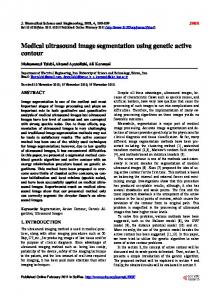
FIG. 1. 共a兲 Hierarchical organization of the tendon 共Ref. 21兲; 共b兲 microstructure of a SDFT CSA showing fiber fascicle bundles and the interfascicular spaces 共Ref. 24兲. Medical Physics, Vol. 37, No. 3, March 2010

1040

Meghoufel et al.: B-scan image simulation, segmentation, and analysis of tendon

II. METHODS II.A. Simulation strategy

II.A.1. Microstructure and B-scan features of the SDFT The SDFT consists of highly specialized connective tissues, which are organized into a hierarchy of structures that include collagen 共main structural protein兲, fibrils, fibers, and fascicles.21–23 As shown in Fig. 1, fibers are arranged in primary fiber bundles. These bundles gather to form secondary fiber bundles 共fascicles兲 and these latter are joined together on the same bundles called tertiary fiber bundles. Fiber bundles are surrounded by a loose connective tissue, called the endotendon or interfascicular space connective tissue, which provides vascular supply, lymphatic vessels, and probably a circular mechanical support. The interfascicular space thicknesses of the tertiary bundles are much bigger than those of the primary and secondary fiber fascicle bundles 关see Fig. 1共a兲兴. The collagen is mainly located at fiber bundle fascicles and it represents 80% of dry weight tendon. Interfascicular space areas are poor in collagen and filled with a fluid consisting mostly of water24 关Fig. 1共b兲兴. The fascicles are regularly parallel to the SDFT loading axis. The main clinical diagnostic criterion to assess the integrity of the SDFT is the B-scan image echogenicity.7,8,12 As described earlier, the B-scan image echogenicity features of a normal SDFT is the presence of parallel and linear hyperechoic structures, when scanning is performed by aligning those structures perpendicular to the U.S. beam 关Fig. 8共a兲兴. It was hypothesized that those structures correspond to the interfascicular spaces,11–13 which are perpendicular to the U.S. wave propagation axis and have thickness values higher than the wavelength. In the case of a lesion, some disorganization of the interfascicular spaces and loss in collagen density occur, resulting in a reduction in the echogenicity11 关Fig. 5共c兲兴. This information was used to design the framework of the simulation model.

1040

euthanized and their SDFTs were excised from the proximal carpal bone in the distal region to obtain a series of macrophotograph slide images representing CSAs. The structural information from those images was later used in simulations to reproduce synthetic B-scans and image structures were compared to those observed clinically. The first step in the macrophotograph image collection process was to embed both SDFT samples directly in a straight phenolic resin solution to create a support around the tendon to facilitate slicing manipulations. Both tendons were cut in 1.3 mm thick CSA slices, regularly spaced using a microtome 共Exakt 300 band system, Oklahoma City, OK兲. On average, 119 共⫾4兲 slices were obtained for each specimen. The CSA aspects of slices were carefully photographed by optical microscopy 共Nikon SMZ-U兲 with a camera 共Nikon HFX DX兲, digitized with a scanner 共HP ScanJet 5590, 200 dpi兲, and stored in a computer. Similar to B-scan images, the successive macrophotograph images were realigned longitudinally by rigid registration.25 Before each acquisition session, a millimetric grid was photographed to set the size of each pixel. Typical images of normal tendon slices are presented in Fig. 2. The dark lines represent the interfascicular spaces and the structures enclosed by it are fascicles. The endotendon junction represents a connection point of many fiber bundles. The standard histomorphometry20 evaluation was performed to quantify the fiber bundle fascicles from the macrophotograph image data set. It consists of an automatic 2D image segmentation followed by a statistical analysis to deduce the average number and the corresponding areas of fiber bundle fascicles for each tendon. Structural measurements showed that the tendon CSA surfaces of the proximal and distal regions were 89.7共⫾4.5兲 and 105.7共⫾4.2兲 mm2, respectively. Interfascicular space thicknesses varied between 54 and 378 ␮m and fiber fascicle bundles appeared as nonclosed structures.

II.A.3. Simulation model: The 2D acoustic wave equation propagation through a SDFT tissue II.A.2. Data collection of B-scan and macrophotograph images of the SDFT Real B-scan images and postmortem macrophotograph slide images of SDFT CSAs were used to support the design of the simulation model. Clinical images were available only in B-scan format and were obtained in vivo from eight normal and five injured horse races at the “École Vétérinaire d’Alfort,” Maisons-Alfort, Val-de-Marne, France. Horse selection was random without taking into account their age and sex. The B-scan of CSAs was acquired from the equine SDFT in free hand mode scanning with a 7.5 MHz linear array transducer 共SSD-2000–7.5 Aloka, Tokyo, Japan兲. Scanning was done along the loading axis direction from proximal to distal regions; free hand speed displacement was around 1 cm s−1. The resulting B-scan image data set totaled 150 共⫾20兲, mean 共SD兲, per horse tendon and realigned longitudinally by rigid registration.25 Two normal animals were Medical Physics, Vol. 37, No. 3, March 2010

The acoustic wave propagation through SDFT tissues was simulated in 2D. A computer software package 共The WAVE2000 PRO, Cyberlogic, Inc., New York, NY兲 computes an approximate solution of the 2D displacement field of the following U.S. 2D wave equation propagation:26

␳

⳵ 2w = ␮ⵜ2共w兲 + 共␭ + ␮兲 ⵜ 共div共w兲兲, ⳵ 2t

共1兲

where ␳ is the volumetric density of each material component of the tissue, ␭ and ␮ are the first and second Lamé coefficients, and w = w共x , y , t兲 are the dynamic 2D displacement field expressed in Cartesian coordinates x and y, where t is time. The symbols ⳵, ⵜ, and div, respectively, denote the partial differential, the gradient, and the divergence operators. The WAVE2000 PRO implements a finite difference technique, as described in Ref. 26.

1041

Meghoufel et al.: B-scan image simulation, segmentation, and analysis of tendon

1041

tion 共i.e., along the U.S. wave propagation axis兲, its size in the lateral direction, and the spatial central frequency. For fully developed speckle, the wavelength ␭ must cover ten nodes in the U.S. wave propagation axis. At f 0 = 7.5 MHz, the corresponding wavelength is about 205 ␮m in the axial direction, ␴x and ␴y have equal sizes and are 2␴y = 2␴x = 5␭ ⬇ 1 mm. The pulse duration was set at 0.5 ␮s. II.B. Image quantification method

FIG. 2. Typical macrophotograph images of a SDFT. The dark lines are the interfascicular spaces and the structures enclosed by the endotendon are fiber fascicle bundles: 共a兲 Proximal CSA; 共b兲 middle CSA; and 共c兲 distal CSA.

II.A.4. SDFT tissue modeling for WAVE2000 PRO implementation As described earlier, the two principal components of normal SDFT are collagen and water. The collagen is mainly located at fiber fascicle bundles and the material within interfascicular spaces and that surrounding the tendon is assumed to be water.24 The WAVE2000 PRO implements a finite differences method to compute an approximate solution of the 2D displacement field.26 The scatterers are considered to be the nodes of the mesh grid of the finite differences method and their spatial locations correspond integrally to pixel locations on the input segmented image 共pixels’ number = nodes’ number兲. A simple thresholding to segment the image presented in Fig. 2共a兲 provides realistic model components of normal SDFT presented in Fig. 3共a兲. CSAs where fibers are disrupted 共pathological cases兲 were modeled as fresh blood 关hemorrhage, white area in Fig. 5共a兲兴. Acoustical properties of collagen, water, and fresh blood were obtained from Refs. 27–29 共Table I兲. As in the clinical acquisition, simulated images of the tendons were produced by implementing with WAVE2000 PRO a 256-element, 7.5 MHz linear array model of the transmit and receive transducer. A single transmit focus of 12 mm from the transducer was used. The excitation pulse was chosen as a Gaussian-modulated sinusoid 共initial boundary condition兲,16 i.e., w共x , y兲 2 2 2 2 = e−.5共x /␴x +y /␴y 兲 sin共2␲ fx兲. ␴x, ␴y, and f, respectively, define the size of the point spread function 共PSF兲 in the axial direcTABLE I. Acoustical parameters of the SDFT components 共Refs. 27–29兲. Parameters ␳, ␭, and ␮ are the volumetric density, first, and second Lamé coefficients, respectively.

␳ in Kg m−3 ␭ in N m−2 ␮ in N m−2

Collagen

Water at 37 ° C

Fresh blood

1100 1235 962

992.63 2241.0 763

1055 2634 833

Medical Physics, Vol. 37, No. 3, March 2010

The SDFT B-scan image processing strategy used by others to quantify image contents has been limited to texture analysis based on the computation of the first-order graylevel statistics 共mean echogenicity兲.8–10,12,14 In the current study, the extraction of fiber bundle was done with a technique that follows the schematic diagram presented in Fig. 7. The stage 1 of the diagram consists in recovering the uncompressed 2D rf envelop signal from the original B-scan image followed by stage 2, in which we perform a combination of 2D binary operations on the recovered 2D rf envelope to extract the real hyperechoic structures. In order to quantify fiber fascicle bundles, we perform a watershed closing operation on the extracted structures to add information in the parallel axis of the U.S. wave propagation. The watershed operation closes the extracted hyperechoic structures 关Fig. 8共d兲兴 without distorting the initial structures of Fig. 8共c兲. II.B.1. Decompression process of B-scan images Clinical U.S. imaging systems employ nonlinear signal processing to reduce the dynamic range of the input rf image to match the smaller dynamic range of the display device and to emphasize objects with weak backscatter. The processing proposed here is based on a method presented in Ref. 19 to derive the approximate unprocessed 2D rf envelope image from 2D B-scan image format. The authors suggested the following intensity transformation: IB = D · ln共I兲,

共2兲

where IB is the available B-scan image format, I is the unknown 2D rf envelope, and D is the mapping parameter. Theoretically, the uncompressed 2D rf envelope intensity I approximately follows an exponential probability distribution for fully developed speckle statistics 共random distribution of a large number of scatterers兲.30 Note that the intensity of the B-scan image IB may follow a different statistical distribution when compression, filtering, and other postprocessing are applied on received echoes, or when scatterers are insufficient and/or not distributed randomly 共coherent scatterers兲.31 Nevertheless, as suggested by Prager et al.,19 the exponential model was considered here because one cannot assume or predict the underlying statistical distribution of received echoes. The approach is to match the measured normalized moments 具In典 / 具I典n of I in a known B-scan region with the expected values for an exponential distribution that is given by ⌫共n + 1兲. The symbols 具 . 典 and ⌫共 . 兲 represent the first statistical moment and the Gamma function, respectively. The mo-

1042

Meghoufel et al.: B-scan image simulation, segmentation, and analysis of tendon

1042

ments are computed for positive values of n, which are not necessarily integers. The algorithm19 proceeds as follows:

closed structures. The quantitative analyses were carried out on fiber bundle number and areas of segmented images.

i. ii.

III. RESULTS

iii. iv.

Choose an initial value for D; Invert the compression mapping for a patch of a known B-scan region using the intensity given by I = exp共IB / D兲; Compute the normalized moments of the intensity data for the powers n = 0.25, 0.5, 1.5, 2.0, 2.5, and 3; and Minimize the mean squared error between the six normalized moments computed and the six normalized moments for an exponential distribution to estimate a value of D.

Knowing D, we can then estimate the uncompressed converted 2D rf envelope intensities I 关see Fig. 8共b兲兴. II.B.2. Binary operations Segmentation of the recovered uncompressed 2D rf envelope image intensities by 2D morphological operations was performed to extract the real hyperechoic structures. The following steps are applied successively: i.

ii.

iii.

The binary operation of Otsu32 on the enhanced image 关Fig. 8共b兲兴 to separate the hyperechoic structures from the background; Closing operation 共dilation followed by erosion operations兲 to fill small holes and to connect contours. The structuring element that was used is a disk with a radius of 5 pixels; and Thinning operation to reduce all lines to a single pixel thickness.

The extracted structures correspond exactly to the real hyperechoic structures observed on the image 关Fig. 8共c兲兴. Some portions of fiber fascicle bundles are widely visible in the perpendicular axis to the U.S. wave propagation; however, no structures are generated in the parallel axis. To compensate the lack of structures in this axis and also to quantify fiber bundle fascicles, we proceed with the watershed closing operation.

II.B.3. Watershed closing operation The watershed closing operation is the appropriate method to close the extracted hyperechoic structures. It adds information in the parallel axis of the U.S. wave propagation 关Fig. 8共d兲兴 without distorting the initial structures 关Fig. 8共c兲兴. The fully validated automatic watershed software 共The IMAGEJ software, NIH, Bethesda, MD, 2009兲 共Ref. 33兲 is used to close the extracted structures. The watershed algorithm is based on binary thickenings with a structuring element of four connected pixels. Figures 8共e兲, 9共a兲, and 9共c兲 show typical results of the proposed imaging technique applied on the clinical and the simulated B-scan images, respectively. The overlay of the extracted contours coincides with the hyperechoic structures of the images. Fiber bundles were defined as the smallest Medical Physics, Vol. 37, No. 3, March 2010

III.A. Simulation model and assessment of its validity

An example of a simulated B-mode image at 7.5 MHz is shown in Fig. 3共b兲. The simulated image contains bright structures drowned in speckle noise. Direct matching between the macrophotograph SDFT tissue model of Fig. 2共a兲 and simulated images revealed that the formed hyperechoic structures correspond to the interfascicular spaces. Moreover, the coherent structure brightness diminishes with their decreasing thickness. Some vertical bright structures are observed 共parallel to the U.S. wave propagation兲; they can be explained by the large thicknesses of the interfascicular spaces in the vertical direction. To further assess the simulation model, namely, to demonstrate the presence of one dominant scattering source with a fairly periodic spatial arrangement representing the interfascicular space structures, we performed the first-order speckle statistics analysis on simulated B-scan images. A Nakagami PDF 共Ref. 31兲 was chosen and its parameters were estimated using the maximum likelihood function.34 Estimate tests showed agreements between the estimated Nakagami PDFs and the real histograms. A typical example of this agreement applied on the area of interest defined in Fig. 3共b兲 is presented in Fig. 3共c兲: The estimated parameter m = 1.64 共shape parameter兲 shows that the echo-texture follows a Rician statistical distribution,31 which indicates the presence of coherent components in the area of interest. This confirms our expectation, since it includes interfascicular space structures. Additionally, to appreciate the realism of simulations and the limited capability of U.S. to resolve small structures, we selected from the histology image of Fig. 2共a兲, two different interfascicular spaces perpendicular to the U.S. wave with different thicknesses E1 ⬵ 300 ␮m and E2 ⬵ 90 ␮m, corresponding to dimensions, respectively, larger and smaller than the acoustic wavelength of 205 ␮m 关see Figs. 4共a兲 and 4共b兲兴. As presented in Fig. 4共c兲, strong bright echoes were obtained from the interfascicular space with thicknesses E1 larger than the wavelength, and no specific structures could be identified for the interfascicular space with thicknesses E2 smaller than the wavelength. III.A.1. Simulation of a pathological SDFT An injured SDFT 共apparition of a lesion兲 is commonly characterized by hemorrhage located in the CSA due to structure disruption.11 To reproduce qualitatively the echotexture pattern of a lesion, a typical histological image 关Fig. 5共a兲兴 was modeled with WAVE2000 PRO to produce a synthetic pathological B-mode image at 7.5 MHz 关Fig. 5共b兲兴. The acoustical properties of the white CSA 关Fig. 5共a兲, fresh blood兴 were obtained from Ref. 29 共Table I兲. The backscattering from the lesion was hypoechoic. As expected, similar hypoechoic features can be observed when compar-

1043

Meghoufel et al.: B-scan image simulation, segmentation, and analysis of tendon

FIG. 3. Simulation result at a 7.5 MHz central frequency: 共a兲 SDFT tissue model of Fig. 2共a兲; 共b兲 simulated B-scan image using the WAVE2000 PRO Model; and 共c兲 measured histogram and the estimated Nakagami PDF in the area of interest identified on panel b.

ing the simulated image with a clinical image that presents a recent injury 关early granulation,10 see Fig. 5共c兲兴. III.A.2. Effect on the insonification frequency on simulations To evaluate changes in the echotexture of normal tendons at different frequencies, simulations were performed at 5, 7.5, 10, and 13 MHz by the proposed simulator 共Fig. 6兲. Echo-textures appeared as internal networks of fine, often parallel and linear bright structures. At higher U.S. frequencies, the interfascicular spaces became clearer and more numerous, had higher reflectivity, and were better separated from one another. Qualitatively, acquisitions at frequencies lower than 7.5 MHz provided indistinguishable structures 关Fig. 6共a兲兴, which can limit the diagnosis of normal versus pathological fiber bundles with the proposed imaging technique. This result corroborates the in vivo assessment of echo-texture changes with frequency reported in Ref. 13.

FIG. 4. Comparison of macrophotography and simulated B-mode structures. 共a兲 Different interfascicular space thicknesses identified by macrophotography; 共b兲 SDFT tissue model structures; and 共c兲 corresponding B-scan image simulated by the WAVE2000 PRO model. Medical Physics, Vol. 37, No. 3, March 2010

1043

FIG. 5. 共a兲 A macrophotography of CSA of the modeled injured SDFT; 共b兲 a simulated B-scan image of an injured SDFT with the WAVE2000 PRO model by considering a 7.5 MHz central frequency; and 共c兲 a clinical B-scan image representing a recent injury, scanned at 7.5 MHz.

III.B. Segmentation results

The proposed image processing was first applied on simulated B-scan images to extract the bright structures from the SDFT CSAs. An example in shown in Fig. 9, the extracted boundaries were projected over the simulated B-scan images 关Figs. 9共a兲 and 9共c兲兴 and over the macrophotography images used to determine the boundaries of the simulation 关Figs. 9共b兲 and 9共d兲兴. As displayed, the extracted contours are very realistic and reflect the hyperechoic versus interfascicular space structures perpendicular to the U.S. beam. However, coarse matching is observed in the parallel axis due to the absence of real structures on the B-scan images.

FIG. 6. B-scan images of a normal SDFT simulated at different frequencies by the Wave 2000 Pro model at 共a兲 5, 共b兲 7.5, 共c兲 10, and 共d兲 13 MHz.

1044

Meghoufel et al.: B-scan image simulation, segmentation, and analysis of tendon

1044

III.B.2. Quantification of fiber bundles on the whole in vivo B-scan data sets Figure 8 shows a segmentation result by the proposed imaging technique applied on a normal clinical B-scan image. A descriptive analysis of fiber bundles for the whole data sets 共eight normal and five injured SDFTs兲 is presented in Table III. The average number of fiber bundles was 50 共⫾11兲 for the normal SDFTs and 40 共⫾7兲 for the injured ones. The corresponding mean areas of fiber bundles were 1.33共⫾0.36兲 mm2 for the normal SDFTs and 1.83共⫾0.52兲 mm2 for injured tendons. In the case of injured SDFTs, fiber bundles were only selected on the intact fascicles. The computed fiber bundle number 共p = 0.016兲 and areas 共p = 0.008兲 were found to be significantly different between normal and injured samples, using student’s t-tests. The determined areas for normal SDFTs agree with in vitro histomorphometric statistics on normal specimens reported by others35 关1.41共⫾0.52兲 mm2兴. IV. DISCUSSION AND CONCLUSIONS FIG. 7. A schematic diagram of the different stages of the proposed imaging technique.

III.B.1. Quantification of fiber bundles on two SDFT simulated specimens Extraction and quantification of fiber fascicle bundles have been applied on the simulated B-scan image database 共around 240 images兲 obtained from the two SDFT specimens. The spatial resolution of those images is a priori known and it was used to set the physical size of closed structures. Values obtained are presented in Table II and they reveal that they are similar to those of the histomorphometry analysis.20 The small variations are potentially caused by the loss of some structures during the image formation, and probably by the watershed operator. The agreement between those values confirms in another way that the targeted hyperechoic structures are caused by coherent specular reflections at the interfascicular spaces observed on the macrophotograph image, and also the accuracy of the proposed imaging technique.

TABLE II. Fiber fascicle bundle number and their corresponding areas computed form two SDFT samples.

Sample #01 Sample #02 Average on both samples

From the simulated B-scan image data set

By histomorphometrya

Number

Number

37⫾ 2 51⫾ 4 44⫾ 8

CSA 2.03⫾ 0.20 1.16⫾ 0.13 1.60⫾ 0.47

a

Reference 20.

Medical Physics, Vol. 37, No. 3, March 2010

32⫾ 5 47⫾ 5 42⫾ 5

Simulation results have identified factors governing the formation of hyperechoic structures on B-scan images. They have also provided information about the relationship between the interfascicular space thicknesses and the wavelength of the U.S. wave propagation in the axial direction. The final aspect of a B-scan image is mainly provided by U.S. reflection and scattering at the interfascicular spaces and by the speckle distribution. Our findings revealed that the interfascicular spaces are most likely responsible for hyperechoic structures on B-scan images. This information corroborates the hypothetic conclusion of previous studies.8–13 The SDFT tissue model can still be improved in order to enhance the realism of simulated images. The next improvement in our model should be the identification of more components than collagen, water, and fresh blood, which are considered as the main SDFT constituents. Simulation results were validated in another way by a statistical analysis of the fiber bundle number and areas on segmented-simulated B-scan images, obtained from two SDFT specimens, which were subject to a standard histomorphometric evaluation.20 The agreement between measured and ground true values confirmed the accuracy of the simulation model. Moreover, the confirmation of the conclusion that hyperechoic structures are caused by the presence of interfascicular spaces was used to extract internal structures and to quantify the integrity of the fiber bundles with our clinical B-scan TABLE III. Fiber bundle number and areas in mm2 关mean 共⫾standard deviation兲兴 for eight normal and five injured SDFTs scanned in vivo. p-values are reported for group differences.

CSA 1.96⫾ 0.32 1.86⫾ 0.32 1.76⫾ 0.60

Normal specimens Injured specimens p-value

N

Fiber bundle number

Fiber bundle areas 共mm2兲

8 5 ¯

50 共⫾11兲 40 共⫾7兲 0.0162

1.33 共⫾0.36兲 1.83 共⫾0.52兲 0.0075

1045

Meghoufel et al.: B-scan image simulation, segmentation, and analysis of tendon

1045

FIG. 10. 3D views of a part of SDFT. Top and longitudinal cuts of tendon: 关共a兲 and 共b兲兴 a normal SDFT; 关共c兲 and 共d兲兴 an injured SDFT. FIG. 8. Fiber bundle structures extraction from a clinical B-scan image by the proposed imaging technique. 共a兲 Original B-scan image; 共b兲 uncompressed 2D rf envelope; 共c兲 binary operations; 共d兲 watershed closing operation; and 共e兲 projection of the closed structures over the original B-scan image.

image data sets. The statistical analysis on fiber bundle number and areas confirmed that our method could objectively discriminate normal from injured SDFTs. The mean fiber bundle number of injured SDFTs was smaller than that of normal ones, and inversely, the mean fiber bundle areas increased for pathological SDFTs 共Table III兲. This clearly indicates the disruption of the thinnest interfascicular spaces and of their corresponding fiber fascicle bundles where lesions occurred.11,13 Fiber bundle areas of the normal SDFTs corroborated values found by histomorphometry on 23 nor-

mal samples35 关1.41共⫾0.52兲 mm2兴. In future works, the fiber bundle number and areas may be used as robust features in a pattern recognition problem to classify healing steps of the SDFT, and to make decisions automatically and accurately when horses recover from tendon injuries. A possible potential use is to provide a commercial 3D imaging software based on the proposed imaging technique to assist the veterinarians during a routine evaluation of tendons. A 3D view can be generated by stacking successiverealigned-segmented images and they can be used to better assess the fiber bundle alignment/distribution along the SDFT loading axis and potential injury locations. Normal and injured SDFTs 共Fig. 10兲 are presented as examples of what veterinarians may visualize to appreciate the integrity of tendons. Images in Fig. 10 were taken from our clinical database. Finally, these results could easily be adapted to the study of human tendons and ligaments. ACKNOWLEDGMENTS This study was supported by the Natural Sciences and Engineering Research Council of Canada 共NSERC Grant Nos. 107998-06 and 138570-6兲, by a National Scientist award of the Fonds de la Recherche en Santé du Québec 共G.C.兲, and by the Chaire de Recherche du Canada en Imagerie 3D et Ingénierie Biomédicale 共J.A.D兲. The authors thank P. Gravel and L. A. Tudor for reviewing this article. a兲

FIG. 9. Extraction of fiber bundle structures from a simulated B-scan image using the proposed imaging technique. Projection of the identified closed structures over the simulated and the macrophotography images of 关共a兲 and 共b兲兴 a normal SDFT; 关共c兲 and 共d兲兴 an injured SDFT. Medical Physics, Vol. 37, No. 3, March 2010

Author to whom correspondence should be addressed. Electronic addresses: [email protected] and [email protected]; Telephone: 共514兲 890-8000 ext: 28720; Fax: 共514兲 412-7785. b兲 Electronic mail: [email protected] c兲 Electronic mail: [email protected] d兲 Electronic mail: [email protected] 1 N. W. Rantanen, “The use of diagnosis ultrasound in limb disorders of the horse,” Equine Vet. J. 2, 62–64 共1982兲. 2 A. Agut, M. L. Martinez, M. A. Sanchez-Valverde, M. Soler, and M. J. Rodriguez, “Ultrasonographic characteristics 共cross-sectional area and relative echogenicity兲 of the digital flexor tendons and ligaments of the metacarpal region in purebred Spanish horses,” Vet. J. 180, 377–383 共2009兲.

1046

Meghoufel et al.: B-scan image simulation, segmentation, and analysis of tendon

3

P. A. Moffat, E. C. Firth, C. W. Rogers, R. K. Smith, A. Barneveld, A. E. Goodship, C. E. Kawcak, C. W. McIlwraith, and P. R. van Weeren, “The influence of exercise during growth on ultrasonographic parameters of the superficial digital flexor tendon of young Thoroughbred horses,” Equine Vet. J. 40, 136–140 共2008兲. 4 C. H. Pickersgill, C. M. Marr, and S. W. Reid, “Repeatability of diagnostic ultrasonography in the assessment of the equine superficial digital flexor tendon,” Equine Vet. J. 33, 33–37 共2001兲. 5 L. J. Zekas and L. J. Forrest, “Effect of perineural anesthesia on the ultrasonographic appearance of equine palmar metacarpal structures,” Vet. Radiol. Ultrasound 44, 59–64 共2003兲. 6 J. C. Gore and S. Leeman, “Ultrasonic backscattering from human tissue: A realistic model,” Phys. Med. Biol. 22, 317–326 共1977兲. 7 J. M. Denoix and V. Busoni, “Ultrasonographic anatomy of the accessory ligament of the superficial digital flexor tendon in horses,” Equine Vet. J. 31, 186–191 共1999兲. 8 H. T. M. van Schie, E. M. Bakker, A. M. Jonker, and P. R. Van Weeren, “Efficacy of computerized discrimination between structure-related and non-structure-related echoes in ultrasonographic images for the quantitative evaluation of the structural integrity of superficial digital flexor tendons in horses,” Am. J. Vet. Res. 62, 1159–1166 共2001兲. 9 H. T. M. van Schie, E. M. Bakker, A. M. Jonker, and P. R. Van Weeren, “Computerized ultrasonographic tissue characterization of equine superficial digital flexor tendons by means of stability quantification of echo patterns in contiguous transverse ultrasonographic images,” Am. J. Vet. Res. 64, 366–375 共2003兲. 10 H. T. M. van Schie and E. M. Bakker, “Structure-related echoes in ultrasonographic images of equine superficial digital flexor tendons,” Am. J. Vet. Res. 61, 202–209 共2000兲. 11 N. Crevier-Denoix, Y. Ruel, C. Dardillat, H. Jerbi, M. Sanaa, C. Collobert-Laugier, X. Ribot, J. M. Denoix, and P. Pourcelot, “Correlations between mean echogenicity and material properties of normal and diseased equine superficial digital flexor tendons: An in vitro segmental approach,” J. Biomech. 38, 2212–2220 共2005兲. 12 T. Garcia, W. J. Hornof, and M. F. Insana, “On the ultrasonic properties of tendon,” Ultrasound Med. Biol. 29, 1787–1797 共2003兲. 13 C. Martinoli, L. E. Derchi, C. Pastorino, M. Bertolotto, and E. Silvestri, “Analysis of echotexture of tendons with US,” Radiology 186, 839–843 共1993兲. 14 C. Gillis, D. M. Meagher, A. Cloninger, L. Locatelli, and N. Willits, “Ultrasonographic cross-sectional area and mean echogenicity of the superficial and deep digital flexor tendons in 50 trained thoroughbred racehorses,” Am. J. Vet. Res. 56, 1265–1269 共1995兲. 15 J. C. Bamber and R. J. Dickinson, “Ultrasonic B-scanning: A computer simulation,” Phys. Med. Biol. 25, 463–479 共1980兲. 16 J. Meunier and M. Bertrand, “Echographic image mean gray level changes with tissue dynamics: A system-based model study,” IEEE Trans. Biomed. Eng. 42, 403–410 共1995兲. 17 V. N. Adrov and V. V. Chernomordik, “Simulation of two-dimensional ultrasonic imaging of biological tissues in the presence of phase aberrations,” Ultrason. Imaging 17, 27–43 共1995兲.

Medical Physics, Vol. 37, No. 3, March 2010

18

1046

G. Haïat, F. Padilla, F. Peyrin, and P. Laugier, “Variation of ultrasonic parameters with microstructure and material properties of trabecular bone: A 3D model simulation,” J. Bone Miner. Res. 22, 665–674 共2007兲. 19 R. W. Prager, A. H. Gee, G. M. Treece, and L. H. Berman, “Decompression and speckle detection for ultrasound images using the homodyned k-distribution,” Pattern Recogn. Lett. 24, 705–713 共2003兲. 20 G. Leblond, N. Crevier-Denoix, S. Falala, S. Lerouge, and J. A. de Guise, “Three-dimensional characterization of the fascicular architecture of the equine superficial digital flexor tendon,” in Sixth International Conference on Equine Locomotion, Cabourg, Normandy, France, 2008 共unpublished兲. 21 J. Kastelic, A. Galeski, and E. Baer, “The multicomposite structure of tendon,” Connect. Tissue Res. 6, 11–23 共1978兲. 22 P. M. Webbon, “A postmortem study of equine digital flexor tendons,” Equine Vet. J. 9, 61–67 共1977兲. 23 P. M. Webbon, “A histological study of macroscopically normal equine digital flexor tendons,” Equine Vet. J. 10, 253–259 共1978兲. 24 C. A. Miles, G. A. Fursey, H. L. Birch, and R. D. Young, “Factors affecting the ultrasonic properties of equine digital flexor tendons,” Ultrasound Med. Biol. 22, 907–915 共1996兲. 25 P. Thevenaz, U. E. Ruttimann, and M. Unser, “A pyramid approach to subpixel registration based on intensity,” IEEE Trans. Image Process. 7, 27–41 共1998兲. 26 R. S. Schechter, H. H. Chaskelis, R. B. Mignogna, and P. P. Delsanto, “Real-time parallel computation and visualization of ultrasonic pulses in solids,” Science 265, 1188–1192 共1994兲. 27 S. A. Goss and F. Dunn, “Ultrasonics propagation properties of collagen,” Phys. Med. Biol. 25, 827–837 共1980兲. 28 P. L. Kuo, P. C. Li, and M. L. Li, “Elastic properties of tendon measured by two different approaches,” Ultrasound Med. Biol. 27, 1275–1284 共2001兲. 29 M. W. Moyer and O. Ridge, Table of acoustic velocities and calculated acoustic properties for solids, plastics, epoxies, rubbers, liquids, and gases, U.S Department of Energy, 1997. 30 R. F. Wagner, S. W. Smith, J. M. Sandrik, and H. Lopez, “Statistics of speckle in ultrasound B-scans,” IEEE Trans. Sonics Ultrason. 30, 156– 163 共1983兲. 31 P. M. Shankar, “Estimation of the Nakagami parameter from logcompressed ultrasonic backscattered envelopes,” J. Acoust. Soc. Am. 114, 70–72 共2003兲. 32 N. Otsu, “A threshold selection method from grey scale histogram,” IEEE Trans. Syst. Man Cybern. 1, 62–66 共1979兲. 33 L. Vincent and P. Soille, “Watersheds in digital spaces: An efficient algorithm based on immersion simulations,” IEEE Trans. Pattern Anal. Mach. Intell. 13, 583–598 共1991兲. 34 C. Julian and N. C. Beaulieu, “Maximum-likelihood based estimation of the Nakagami m parameter,” IEEE Commun. Lett. 5, 101–103 共2001兲. 35 C. Gillis, R. R. Pool, D. M. Meagher, S. M. Stover, K. Reiser, and N. Willits, “Effect of maturation and aging on the histomorphometric and biochemical characteristics of equine superficial digital flexor tendon,” Am. J. Vet. Res. 58, 425–430 共1997兲.