Understanding robustness in Random Boolean Networks Kai Willadsen1,2 , Jochen Triesch1 and Janet Wiles2,3 1
Frankfurt Institute for Advanced Studies, Johann Wolfgang Goethe University, 60438 Frankfurt am Main, Germany 2 School of Information Technology and Electrical Engineering, University of Queensland, QLD 4072, Australia 3 ARC Centre for Complex Systems, School of Information Technology and Electrical Engineering, University of Queensland, QLD 4072, Australia
[email protected] Abstract
robustness in large networks of interacting elements—such as genetic regulatory networks—can result from simple parameterisation, rather than being a property which must be designed or evolved. In addition, the connectivities at which RBNs display interesting and robust behaviour closely parallel the connectivities found in real-world genetic regulatory systems (Kauffman, 1969; Aldana, 2003).
Long used as a framework for abstract modelling of genetic regulatory networks, the Random Boolean Network model possesses interesting robustness-related behaviour. We introduce coherency, a new measure of robustness based on a system’s state space, and defined as the probability of switching between attraction basins due to perturbation. We show that this measure has both upper and random-case bounds, and that these bounds are based on the size of individual attractor basins within the system. A mechanism for calculating these bounds is introduced, and the bounds are then used to define structural coherency, a measure of robustness attributable to system structure. Using these measures, we show that the decrease in coherency that occurs in the Random Boolean Network as its connectivity increases is related to a loss of structure in the system’s state space.
A mix of theoretical (Derrida and Pomeau, 1986; Derrida and Flyvbjerg, 1987) and simulation-based (Kauffman, 1969; Aldana, 2003; Bastolla and Parisi, 1997) approaches have previously been used to understand the behaviour of robustness in RBNs. The most common technique used in theoretical analysis of discrete dynamic systems such as RBNs is the annealed approximation model (Derrida and Pomeau, 1986) which provides an analytically tractable approximation of RBN behaviour. This framework provides a useful theoretical prediction of the behaviour of infinite ensembles of networks under certain restrictive assumptions. However, this approach cannot be used to investigate single instantiations of the RBN model, or functional models of real-world systems. In contrast to the theoretical approach, simulation-based approaches are based upon the collection of metrics from multiple individual systems (Bastolla and Parisi, 1997; Aldana, 2003; Wuensche, 1998). As such, these approaches can be used to investigate robustness of individual networks in order to provide information about the range of behaviours observed under different circumstances, rather than just behavioural averages. So far, however, both theoretical and simulation-based approaches have generally focused on characterising the properties associated with robustness in the system (such as the areas of parameter space in which robustness is generally found), without focusing on understanding what system-level properties bring about the occurrence of robustness or lack thereof.
Introduction Since the introduction of the Random Boolean Network (RBN) model as a framework for modelling genetic regulatory networks (Kauffman, 1969), the robustness of the model has been an area of considerable research (Kauffman et al., 2003; Luque and Sol´e, 1998). This interest is due in part to the importance of understanding how robustness emerges in regulatory systems, and in part to the general applicability of the RBN model as a basis for understanding the dynamics of complex systems with epistatic interactions. Studies of the spontaneous emergence of robustness in the model have led to a greater understanding of the way in which robustness can be maintained in complex systems, as well as a better comprehension of what it means for a system to be stable. Informally, robustness can be thought of as a system’s ability to function normally under external perturbations. The investigation of robustness in RBNs generally focuses on the dependence between robustness and network connectivity. This focus sources from the discovery that the robustness of a RBN undergoes a phase transition around an average network connectivity of two (K = 2) (Kauffman, 1969). Later supported by theoretically based approaches (Derrida and Pomeau, 1986), this property demonstrates that
Artificial Life XI 2008
In this study, we define a new robustness metric we call coherency, which is based on the full enumeration of a system’s state space. We use a combination of simulation-based and theoretical approaches to identify the relationship between the size of a system’s basins of attraction and system coherency, as part of understanding the way in which robust-
694
ness arises in the RBN model. In addition, the formulation of coherency as a measurable property of individual systems means that coherency may be useful in characterising robustness in existing models of real-world systems.
Random Boolean Networks and state spaces A RBN consists of N nodes or elements, each of which has exactly K incoming connections from other network nodes, and an average of K outgoing connections to other nodes in the network. Each node n in the network has a Boolean value σn which changes over time depending on a random Boolean function fn of the inputs to the node (i.e., σn (t + 1) = fn (σn1 (t), . . . , σnK (t)), where σni indicates the ith input to node n). The Boolean function associated with an individual node is independently randomly generated for each node, and stays constant over the lifetime of a system. RBNs are discrete dynamic systems: discrete because each node in a system has a discrete value; and dynamic because the value of individual nodes changes over time. Boolean-valued nodes imply that the system has a finite number of states (2N ). In addition, the unchanging (or quenched) nature of the random Boolean functions f1 . . . fN means that the model is also deterministic. One way of conceptualising the dynamics of a system is through the system’s state space. State space consists of the set of all possible states of the system, and the set of state transitions (system dynamics) defined by the collective action of the random Boolean functions f1 . . . fN . Graphically, states in the system can be represented as nodes in a graph, with edges between nodes representing state transitions (see Figure 1). In a RBN, this state space will have points or limit-cycles (here referred to collectively as attractors) consisting of one or more nodes which define the dynamic behaviour of the system in the time limit; any system running indefinitely must end up in an attractor. The length of an attractor is the number of nodes in the attractor’s cycle. In addition, associated with each attractor is a set of states which lead to that attractor, termed the basin of attraction. The size of a basin of attraction is the number of states in the basin; alternatively, size can be expressed as basin weight, being the proportion of state space occupied by the basin’s states. For example, Figure 1 shows a RBN state space (N = 8, K = 6) with three attractors of length 3, 7 and 19 and three corresponding basins of attraction with 94 142 20 ), 94 (weight 256 ) and 142 (weight 256 ). size 20 (weight 256 Attractors and basins of attraction are important concepts in defining the robustness of individual RBNs, as they represent the deterministic dynamics of a system leading to its steady state.
Figure 1: An example RBN state space graph with N = 8 and K = 6 containing three attractor basins. Nodes in the graph represent states of the network, with directed edges representing the state transitions determined by the Boolean functions of the network.
simulation-based perturbation methods. The annealed approximation framework, which is applied in the context of a statistical ensemble of systems, uses a theoretical method to determine the probability of state perturbations propagating through a system (Derrida and Pomeau, 1986). In this framework, robustness is defined as the probability that a perturbation to the activation of a node will, over time, spread to affect other nodes in the network. A stable network is one in which a perturbation to the state of the network at time t will likely result in the same network state at time t+∆t (i.e., the perturbation dies out). If the states of the perturbed and unperturbed network differ at time t+∆t, then the network is considered unstable (i.e., the perturbation has spread). The second method for measuring robustness is a simulation-based random-sampling approach that is best described as ‘perturb and iterate’. In this approach, robustness is defined as the probability of a single-element perturbation to a system state s resulting in a system state s0 that is in the same basin of attraction as the original state (Aldana, 2003; Geard et al., 2005; Reil, 1999). These two measurements of robustness are closely related, both defining robustness as a lack of change of network expression in the time limit. However, both of these measurements have different shortcomings. The annealed approximation approach cannot be used to describe individual RBNs, meaning that it is not useful for analysing models of specific real-world systems. In contrast, the ‘perturb and iterate’ approach is based on random sampling, which only provides an incomplete—and possibly inaccurate—picture of a system’s robustness. In this study, we define a measure closely related to the above approaches, which we term coherency, based on the full-enumeration of a system (i.e., generating every possible
Defining coherency There are two commonly used approaches to measuring robustness in RBNs: annealed-approximation methods; and
Artificial Life XI 2008
695
system state and identifying each state’s successor). The coherency of a system is defined to be the probability that a single-element perturbation to any state of the system does not change the basin of attraction of the state. As a codification of robustness, coherency characterises a system as robust if a small perturbation to the system state is unlikely to affect the long-term behaviour of the system. Coherency can be most simply defined in terms of an individual state. For a state s with neighbouring states nh (where neighbouring states are states that differ by only a single element; i.e., states having a Hamming distance to s of one), the coherency of that state ψs is the percentage of states nh that are in the same basin of attraction as s. This definition can be readily extended to arbitrary collections of states, the most interesting of which are whole systems, and attractor basins. For a system S we define the system coherency ψS , 1 X ψs , (1) ψS = |S|
100%
Average basin coherency
Coherency
80%
60%
40%
20%
0% 0
2
4
6
8
10
12
14
16
Connectivity (K)
Figure 2: Coherency vs. connectivity for whole state spaces and individual basins of attraction in RBN systems (N = 16; error bars show standard error). System coherency (ψS ) and basin coherency (ψ¯B ) both fall as connectivity increases, with basin coherency falling more rapidly.
s∈S
where s ∈ S are individual states of the system, and ψs are coherencies of individual states. As the coherency of any group of states is the average of the coherency of each individual state, we can also formulate the coherency of a system as the average of the coherencies of its basins of attraction, weighted by the size of each basin, X |b| ψS = ψb N , (2) 2
model was simulated (N = 16, K = 1, 2, 3, 4, 8, 16; 1000 trials). For each trial, the system coherency ψS and Pthe av1 erage of individual basin coherencies ψ¯B = |B| b∈B ψb were recorded and averaged over each parameter combination. The coherency of whole systems is seen to decrease as connectivity increases (see Figure 2), which agrees with accepted knowledge about the robustness of RBNs (Aldana, 2003). However, this result does not provide any insights as to the mechanisms causing coherency in systems with low connectivity, or those underlying the loss of coherency in higher-connectivity systems. For these insights we must consider the coherency of sub-structures of the system’s state space: attractor basins. The average coherency of basins of attraction in a system is also seen to decrease as K increases (see Figure 2), but this decrease is far more rapid than the corresponding decrease in the overall system coherency. These results can be explained in terms of the relationship expressed by (2), by observing that it is the interaction between coherency and weight of individual basins of attraction that is crucial in determining system coherency. Given this relationship, the difference between the decrease in basin coherency and system coherency suggests that not every basin of attraction contributes equally to overall system coherency. In order to understand the transition between stable and chaotic regimes in the RBN model, as characterised by a changing system coherency, we need to understand the relationship between coherency and size of attractor basins within a state space. This relationship may be characterised by comparing the size of each basin of attraction with the basin’s coherency, and observing how these values change
b∈B
where B is the set of attractor basins of the system, and |b|/2N is the weight of an individual basin. The computational complexity of measuring coherency is prohibitive, being O(N 2N ) in both time and space, but is nevertheless feasible for small systems (N ≤ 25); even at such a restricted system size, this measure is applicable to both abstract systems such as RBNs and interesting models of real-world systems (e.g., Albert and Othmer, 2003; Li et al., 2004; Mendoza and Alvarez-Buylla, 1998). In exchange for this computational complexity, coherency avoids the drawbacks associated with existing robustness measures for RBN systems: unlike the annealed approximation approach, coherency measures specific individual systems; and unlike the ‘perturb and iterate’ approach, it tests all possible single-element perturbations for all system states. In addition, the definition of coherency is general in that it can be applied to any collection of states simply by considering only a subset of system states. In other words, coherency, as defined here, is a comprehensive measurement of the robustness of an individual system or parts of the system.
Basin coherency, basin size and network connectivity In order to understand this new measure of robustness, and to see what information it may provide, the standard RBN
Artificial Life XI 2008
Average system coherency
696
with respect to the connectivity of the system, K. The relationship between coherency and basin size does exhibit a change as the value of K increases, from an apparently logarithmic relationship to a linear one (see Figure 3). Just as one notable characteristic of the data is the variance of this relationship with K, another pertinent characteristic is the apparent restrictions on the upper and lower values of basin coherency with respect to basin weight. Making use of known properties of the RBN model, we can investigate the observed upper and lower bounds on the relationship between coherency and basin size.
100%
Basin coherency
80%
Random-case bounds on coherency
|b| − 1 . 2N − 1
K4 40%
K2
0% 0%
20%
40%
60%
80%
100%
Normalised basin size
Figure 3: Basin weight vs. basin coherency for N = 12 and K = 2, 4, 12. The three connectivity levels demonstrate a clear separation. At low K, the data describes a curve that is significantly above the identity line, with the relationship tending toward linear as K increases.
As the K → N limit is the least stable point in the parameter space of a RBN (Bastolla and Parisi, 1997), (3) can be taken as a random-case probabilistic bound of the coherency of any RBN system, and a description of the lowest sizecoherency pairs that are likely to be observed.
Upper bound on coherency Determining the upper bound on the coherency of a basin of attraction is not readily amenable to an analytic solution. A simulation-based approach was therefore undertaken to investigate the way in which formation of highly stable basins of attraction occurred in RBN systems. Since K = 1 is the most stable point in the RBN model (Flyvbjerg and Kjær, 1988), an investigation of the structure of attractor basins in these systems was undertaken. The structure of the state spaces investigated was analysed using schemata to represent the states present in a basin of attraction. The state of a Boolean network model can be represented by a vector of Boolean elements (e.g., [ 1 0 0 1 0 ] would be a state in an N = 5 system); using a ternary representation—a schema—with elements ‘0’, ‘1’ and a wild-card, ‘?’, makes it possible to represent many states in a compact fashion (Bagley and Glass, 1996). It was discovered that representing basins of attraction in this manner provided insights into the formation of highly coherent basins of attraction in low K systems. Highly coherent basins of attraction in these systems could generally be described by a very simple schema. For
(3)
As the coherency of each individual state in a basin can be seen as a Bernoulli trial, basin coherencies from completeenumeration simulations will be binomially distributed with, |b| − 1 , 2N − 1 n = N |b| . p=
1
While there is an actual lower bound on coherency defined by a parity function, this bound does not correspond to any known parameterisation of the RBN model.
Artificial Life XI 2008
K 12
20%
In the RBN model, it is expected that the lower bound on the observed coherency will occur when the system is most highly disordered1 , a condition that occurs at maximum network connectivity. This lower bound on the observed relationship between coherency and basin size, referred to here as the random-case bound, is a probabilistic bound that describes system behaviour over a statistical ensemble of systems. The random-case bound occurs as K → N , and is a linear relationship between the weight and the coherency of the attractor basin. It has been shown that for N → ∞, K → N , RBNs correspond to the random map model (Derrida and Flyvbjerg, 1987). In this model, the system dynamics implement a random mapping between states in the system. That is, given a state s, the system’s dynamics define a transition that will deterministically move the system to a new state, s0 ; in the random map model, the target state, s0 , is randomly assigned for all such transitions. It follows that since there is no correlation between a state and its successor, there is also no correlation between the states in an attractor basin, since the basin is defined by these transitions. If there is no correlation between states in a basin of attraction, then the expected coherency—the probability of the result of a single-point perturbation belonging to the same basin of attraction—is proportional to the weight of the basin of attraction. After accounting for the fact that a perturbation cannot result in the original state, we have, ψrand (b) =
60%
697
example, a basin that covered exactly half of the state space of a five-element system could be described by a schema such as [ ? ? 0 ? ? ]. That is, the basin would be formed by making membership of the basin contingent on the value of a single element in the system. Similarly, a basin covering one quarter of the state space would be contingent on the value of two elements, and so on. In cases where a basin was of a size that could not be described by a single schema, basins were generally found to be composed of simple, non-overlapping schemata whose sizes formed a minimum binary partition of the basin size. For example, a basin of size 715 would likely be composed of six non-overlapping basins with sizes 512, 128, 64, 8, 2 and 1. Given these observations, we conjecture that the upper bound on the robustness of a basin of attraction exists when the basin is composed of a set of non-overlapping schemata, I, with sizes corresponding to a minimum binary partition of the basin size. In other words, the set I satisfies the equation, X |b| = |i| , (4)
100%
Coherency of basin
80%
0%
20%
40%
60%
80%
100%
Size of basin (%age of space)
Figure 4: The conjectured upper (solid) and random-case (dashed) bounds on the expected coherency of a basin of attraction for an N = 12 system.
As N increases, the maximum possible coherency for a given basin weight (%age size) increases. In other words, a basin that occupies 20% of an N = 50 state space has a higher maximum coherency than a basin occupying 20% of an N = 10 state space (see Figure 5). This increase is most notable for relatively small basin sizes.
j∈(I\i)
(5) where I is the set of schema sizes described above, and N is the size of the network. The sum over I \ i represents the coherency between the schema with size i and the other schemata in I. Since I is determined solely from the basin size, and is unique for any given value thereof, our conjectured upper bound (referred to below simply as the upper bound) can be calculated from the size of the network, N , and the size of the basin, |b|. The conjectured upper and random-case bounds outline the area in which relationships between coherency and basin size are expected to fall within the gamut of RBN systems (see Figure 4). Like the random-case bound described above, this upper bound is not a theoretical limit describing the maximum possible coherency of a basin of attraction of the given size, but rather a bound on the expected coherency, based upon an analysis of observed system behaviour. Nevertheless, numerical simulations indicate that this bound is a useful approximation (see following section). An interesting property of the upper bound is its change with respect to N . The coherency of a basin of attraction b of size |b| can be approximated by,
Artificial Life XI 2008
Random coherency
40%
0%
and is the smallest set to do so. The constraints placed upon this set (i.e., that each number in the set is unique, that each number is a power of two, and that the schemata are nonoverlapping) mean that it is possible to calculate an optimal coherency from I alone (see appendix). The maximum coherency of a basin ψmax is given by, X X |i| 1 log2 |i| + , ψmax (I, N ) = N |b| d|i| ÷ |j|e
log2 |b| . N
Maximum coherency
20%
i∈I
i∈I
60%
Testing bounds The upper and random-case bounds developed above (see Figure 4) appear to provide useful and accurate bounds on the observable coherencies of basins of attraction (see Figure 6). As a simple measure of the accuracy of the predictions, we can investigate the frequency with which the bounds are violated (see Table 1). In all simulations, the upper bound described a hard upper limit on the relationship between coherency and basin size. While attractor basins with coherency-size pairs below the random-case bound were found, this is to be expected as described above.
Attributing robustness to structure The upper and random-case bounds on expected coherency relate basin robustness to basin structure; unstructured basins have notably lower robustness than structured basins, given equality of size. However, since we can determine the maximum and random-case robustness for any given basin size, we can also quantify the degree to which an attractor basin’s robustness depends on its structure rather than its size. By comparing the actual coherency of a basin to the maximum and random-case coherency, we can express basin
(6)
698
100%
100%
80%
80% N 20
Coherency of basin
Coherency of basin
N 50 N 10
60%
40%
Coherency predictions
60%
K=12 K=8 40%
K=4 K=2 K=1
20%
20%
0%
0% 0%
20%
40%
60%
80%
Size of basin (%age of space)
100%
0%
20%
40%
60%
80%
100%
Size of basin (%age of space)
Figure 5: The change in the maximum possible coherency of a basin of attraction of a given normalised size with respect to N . As N increases, the coherency of an absolute basin size remains the same, but the coherency of the relative basin size increases. As N becomes large, even basins that are very small relative to the state space may be highly coherent.
Figure 6: Observed coherencies for RBN systems (N = 12; K = 1, 2, 4, 8, 12; 50 trials). The various observations fall largely within the shaded area, which represents the expected boundaries; due to the probabilistic nature of the random-case bound, some data points are found below the expected boundary.
robustness as a proportion of the difference between sizedependent and maximum robustness. This measure, which we term structural coherency, can be expressed as ψstruct ,
coherency, structural coherency seems to be approximately constant over basin size, while still varying as expected over K. This measurement shows that even in small basins of attraction, the basin structure within low K systems results in attractor basins with high relative degrees of coherency.
ψstruct (b) =
ψ(b) − ψrand(b) . ψmax (b) − ψrand (b)
(7)
Conclusions
Structural coherency has no meaningful interpretation for basin sizes with the same maximum and random-case coherencies: 1, 2N − 1, and 2N . Measuring the structural coherency of RBNs with varying connectivity, we obtain a clear striated pattern showing structural coherency progressing from 100% to 0% as K increases from 1 to N (see Figure 7). In contrast to normal K
Lower
Within
Higher
1 2 4 8 12
0.0% 0.0% 0.6% 10.5% 43.6%
100.0% 100.0% 99.4% 89.5% 56.4%
0.0% 0.0% 0.0% 0.0% 0.0%
Robustness or lack thereof in individual RBNs can be analysed in order to better understand when and how robustness arises. We have demonstrated a combination of simulationbased and simple theoretical techniques to provide information about the relationship between the robustness of a system and the size of individual attractor basins within that system. It was suggested that basins of attraction in a system have both upper and random-case bounds on their coherency that depend only on the size of the basin of attraction and the size of the system as a whole. In isolating the maximum and random-case coherency values for a particular system, the concept of structural coherency was established to describe the proportion of basin robustness attributable to the structured organisation of a state space. These measures may subsequently be used in order to try and identify causal relationships between robustness and other system properties, such as network architecture or environmental influences (Willadsen and Wiles, 2007).
Table 1: Percentage of attractors that were below, within or above the bounds (N = 12; K = 1, 2, 4, 8, 12; 50 trials). The frequency of overstepping the random-case bound is consistent with the probabilistic nature of that bound.
Artificial Life XI 2008
699
Structural coherency of basin
References Albert, R. and Othmer, H. G. (2003). The topology of the regulatory interactions predicts the expression pattern of the segment polarity genes in Drosophila melanogaster. Journal of Theoretical Biology, 223(1):1–18.
100% 80% K 16
60%
K8
Aldana, M. (2003). Boolean dynamics of networks with scale-free topology. Physica D, 185:45–66.
K4
40%
K2 K1
20%
Bagley, R. J. and Glass, L. (1996). Counting and classifying attractors in high dimensional dynamical systems. Journal of Theoretical Biology, 183:269–284.
0% 0%
20%
40%
60%
80%
100%
Bastolla, U. and Parisi, G. (1997). A numerical study of the critical line of Kauffman networks. Journal of Theoretical Biology, 187:117–133.
Size of basin (%age of space)
Figure 7: Observed structural coherencies vs. basin size (N = 16; K = 1, 2, 4, 8, 16; best-fit lines indicated). Structural coherency appears to be approximately constant over basin size, but varying over K.
Derrida, B. and Flyvbjerg, H. (1987). The random map model: a disorded model with deterministic dynamics. Journal de Physique, 48:971–978.
The network connectivity of the RBN model, K, was shown to affect the coherency of a system by changing both the size and coherency of basins of attraction. The relationship between basin coherency and basin size for basins of attraction in K = 1 and K = N systems demonstrated strong agreement with the upper and random-case bounds respectively. The structural coherency of attractor basins was shown to be indirectly proportional to the network connectivity, demonstrating that chaotic (high connectivity) networks have low robustness because their state space becomes disorganised. A notable difference in the results provided by coherency and other robustness measures (e.g., Kauffman, 1969; Derrida and Pomeau, 1986) is that the coherency results show no special phase-transition behaviour at K = 2. From these results, we believe that it is possible to understand how, why and under what conditions robustness occurs in discrete dynamic systems such as Random Boolean Networks, and in discrete dynamic models of real world systems. While the methods presented here do not scale well (i.e., O(N 2N )), several pre-existing interesting, small-scale models of real-world biological systems (e.g., Albert and Othmer, 2003; Li et al., 2004; Mendoza and Alvarez-Buylla, 1998) are amenable to such analysis (Willadsen and Wiles, 2007). Understanding such model systems may eventually help in the analysis of robustness in real-world systems, such as developmental robustness and homeostasis in genetic regulatory networks.
Flyvbjerg, H. and Kjær, N. J. (1988). Exact solution of Kauffman’s model with connectivity one. Journal of Physics A: Mathematical and General, 21(7):1695–1718.
Derrida, B. and Pomeau, Y. (1986). Random networks of automata: A simple annealed approximation. Europhysics Letters, 1(2):45–49.
Geard, N., Willadsen, K., and Wiles, J. (2005). Perturbation analysis: A complex systems pattern. In Abbass, H., Bossamaier, T., and Wiles, J., editors, Recent Advances in Artificial Life, volume 3 of Advances in Natural Computation, pages 69–84. World Scientic Publishing, Singapore. Kauffman, S., Peterson, C., Samuelsson, B., and Troein, C. (2003). Random Boolean network models and the yeast transcriptional network. PNAS, 100(25):14796–14799. Kauffman, S. A. (1969). Metabolic stability and epigenesis in randomly constructed genetic nets. Journal of Theoretical Biology, 22:437–467. Li, F., Long, T., Lu, Y., Ouyang, Q., and Tang, C. (2004). The yeast cell-cycle network is robustly designed. Proceedings of the National Academy of Sciences, 101(14):4781–4786. Luque, B. and Sol´e, R. V. (1998). Stable core and chaos control in random Boolean networks. Journal of Physics A, 31(6):1533–1537. Mendoza, L. and Alvarez-Buylla, E. R. (1998). Dynamics of the genetic regulatory network for Arabidopsis thaliana flower morphogenesis. Journal of Theoretical Biology, 193(2):307– 319. Reil, T. (1999). Dynamics of gene expression in an artificial genome - implications for biological and artificial ontogeny. In Floreano, D., Nicoud, J.-D., and Mondada, F., editors, Fifth European Conference on Artificial Life. Willadsen, K. and Wiles, J. (2007). Robustness and state-space structure of Boolean gene regulatory models. Journal of Theoretical Biology, 249:749–765.
Acknowledgements
Wuensche, A. (1998). Discrete dynamical networks and their attractor basins. In Standish, R., Henry, B., Watt, S., Marks, R., Stocker, R., Green, D., Keen, S., and Bossomaier, T., editors, Complex Systems ’98.
The authors would like to acknowledge Nic Geard, Jennifer Hallinan, Ben Skellett and James Watson for useful discussion. The Pajek software package was used in the production of graph visualisations.
Artificial Life XI 2008
700
Appendix: Calculating conjectured upper bound coherency
Determining coherency between two individual schemata can be accomplished by some simple logic. Given that the conditions for maximum coherency state that the collection of schemata is minimal, and that schemata are non-overlapping, we can divide the coherency calculation into two disjoint conditions: |i| > |j| and |i| < |j|. When |i| > |j|, the probability that a perturbation of i will lead to j is dependent on the relative sizes of i and j. The total number of possible perturbations from schema i is N |i|, and the number of target states is |j|, implying coh(i, j) = N|j||i| . When |i| < |j|, we rely upon the hierarchical nature of the schemata; membership of each schema is determined solely by the value of a single element. Therefore, changing from a smaller schema, i, into a larger schema, j, implies perturbing the single appropriate element in a system of N elements, thus coh(i, j) = N1 . Combined, we can write,
We have conjectured that the upper bound on basin robustness is characterised by a basin being composed of a set of schemata I, such that the schemata i ∈ I are non-overlapping, and have sizes that correspond to a minimum binary partition of the basin size. Here we calculate the relationship between basin size and basin coherency under these conditions. Each schema comprising a basin of attraction makes a coherency contribution proportional to the size of the schema, in the same way that basins of attraction make coherency contributions to a system. The coherency of a single schema is equal to the probability of a perturbation resulting in a state that is in the schema, coh(i, i), added to the probability of a perturbation resulting in a state that is outside the schema, but is in another schema in the same basin of attraction coh(i, I \ i). Therefore, ” X |i| “ ψmax (I) = coh(i, i) + coh(i, I \ i) . (8) |b| i∈I
coh(i, j) =
log2 |i| , N
coh(i, j) =
(9)
,
(11)
1 . N d|i| ÷ |j|e
(12)
Combining (8) and (12) yields an equation for the maximum expected coherency of a system with N network nodes, and attractor basin sizes I, 0 1 X |i| X 1 @log2 |i| + A . ψmax (I, N ) = N |b| d|i| ÷ |j|e i∈I
x
where |i| is the schema size, being 2 where x is the number of wild-card elements in i. The coherency of the schema i with all other schemata in the basin is the sum of the coherency of schema i with each individual schema j ∈ I \ i. Denoting this coherency as coh(i, I \ i), we have, X coh(i, I \ i) = coh(i, j) . (10)
j∈(I\i)
(13)
j∈(I\i)
Artificial Life XI 2008
if |i| < |j| if |i| > |j|
or alternatively,
The coherency of the schema i with itself is simply the size of the schema, normalised with respect to the system size. Denoting the self-coherency as coh(i, i), coh(i, i) =
1 N |j| N |i|
701