When designing a field of passive underwater sensors, a series of assumptions are typically made, with one of the more glaring being range independence ...
UNDERWATER SENSOR FIELD DESIGN USING GAME THEORY Erik F. Golen and Nirmala Shenoy Rochester Institute of Technology Rochester, NY and Bruce Imre Incze Naval Undersea Warfare Center Division Newport Newport, RI ABSTRACT When designing a field of passive underwater sensors, a series of assumptions are typically made, with one of the more glaring being range independence throughout an operational area. It is unlikely that a large water space will have uniform acoustic characteristics, meaning that the performance of a sensor will vary based on its physical location. Considering that a threat may also have knowledge of the acoustics of an area, a field designer could divide the area into sectors based on changes in acoustics and predict how often a threat submarine will visit each sector of the area to increase the field’s submarine detection capabilities. In this work, an operational area is split up into four quadrants with varying acoustic characteristics and the probability of visitation to each quadrant by a threat submarine is determined using game theory. A new Game Theory Field Design (GTFD) model is proposed that properly allocates sensors to each quadrant according to the visitation probabilities. When compared with a random field design model that does not consider these probabilities, GTFD is shown to offer a significant improvement in terms of detection capability. I. INTRODUCTION Designing a field of passive underwater sensors is a daunting task due to the voluminous areas that need to be well protected from stealthy enemy submarines given a fixed number of sensors to use and changes in acoustic characteristics within the area. The purpose of these fields may range from protecting a valuable asset such as a fuel ship to surveillance of a crucial water space. Over time, sensor deployment has been attempted using a number of different techniques wherein a few strong assumptions commonly occur, three of which will be focused on in this work. The first assumption is that of a centralized highpowered communication node within a sensor field, as used in [2]. The purpose of this node is to act as a single sink for the entire sensor field where all sensors send their data. It aggregates all of the sensor data and sends it out to 1-4244-1513-06/07/$25.00 ©2007 IEEE
a central location such as an unmanned air vehicle or a ship. This assumption is inadequate because of the strain that will be put on the nodes in the sensor field. In such a field, sensors are forced to not only sense, but also, to continually route data from other sensors towards the centralized sink, potentially consuming much of the sensor’s limited battery power on a function it was not intended to almost exclusively perform. Additionally, the placement of sensors is restricted since there must always exist a path from every sensor to the sink, meaning that clusters of sensors can never be segmented from the rest of the sensor field. Not allowing segmentation could prevent outlying sectors of an area from being covered with sensors due to an inability to create a path to the sink. The second and third assumptions include the range independence in both sensing and communication range, regardless of a sensor’s location. Sensing range implies the range in which a sensor can sense a phenomenon, while communication range defines the range in which a sensor can communicate with another sensor. These two assumptions normally cannot hold since underwater sensing and communication ranges vary as a function of the acoustic characteristics at their location, or in other words, are range dependent [5]. For example, in [3] and [4], fields are created using sensors with constant sensing range to minimize the probability that a target goes undetected if the target follows a maximal breach path. This path denotes the path a target can take that allows it to have the greatest chance of not being detected by the field. If this methodology were used in an environment where the sea bottom suddenly slopes down and the assumption was that the sensing range is the same throughout the area, the sensors on the slope would not perform as expected. Hence, to assume range independence, as is done in [2-4], may invalidate the results gathered about a sensor field’s sensing and communication coverage in underwater sensor networks. Rather than assuming the existence of a single centralized sink node and sensing range independence, a new Game Theory Field Design (GTFD) model is proposed that
1 of 7
relaxes these assumptions to create sensor fields that will be more effective in practice than those using these assumptions, while applying concepts from game theory to take advantage of the effect of range dependence on the behavior of a threat submarine. Resulting from the GTFD model is a field that considers the probability of visitation of a submarine to sectors of a field, based on the acoustic characteristics within the field. Analysis and simulation results show that the proposed GTFD is superior to fields created using a random field design method. The remainder of this paper is organized as follows. A short discussion of underwater acoustics and search will be given in Section II, followed by a presentation of the game theory used in GTFD in Section III. The GTFD model and a competing model will then be shown in Section IV. In Section V, the two models will be compared analytically validated via simulation. Finally, a discussion of the analytical results will be given in Section VI and a series of conclusions drawn in Section VII.
the farthest away cell with a non-negative signal excess is considered to be the sensing radius of a sensor in that quadrant. Only two of the five terms in Equation 1 are directly affected by the location of the sensor, the transmission loss TL and the noise level NL. Transmission loss, indicative of a quadrant’s acoustic characteristics, refers to the weakening of a signal with range as a result of its propagation through the water. This loss varies based upon factors such as bottom depth and sounds speed. The noise level consists of both noise that is a result of the sensor being used and ambient noise in the environment [5]. All of the remaining terms are essentially constants with source level SL being the level of sound emitted by a threat submarine, directivity index DI acting as a gain for the sensor based on how well it can determine the direction sound is coming from, and detection threshold DT representing the level of sound required to differentiate the target from the medium.
II. ACOUSTICS AND SEARCH In this study, without loss of generality, an operational area will be divided up into four distinct quadrants, for simplicity, each having different acoustics from the other, but the acoustics of each quadrant is uniform, not random, within its boundaries. Based on these acoustics and a number of passive sensors available to a field designer, a probability of visitation by a threat submarine to each quadrant can be derived using game theory. Using these probabilities, a number of sensors will be placed in! each area to maximize the detection capabilities of the intruding adversary. To create the game, the sensing radius of a sensor in each quadrant must first be determined using the Passive Sonar Equation [5].
SE = SL ! TL + DI ! DT ! NL
(1)
In this equation, SE is the signal excess at a particular location, or grid cell, with respect to the location of a sensor where a grid cell is a small subdivision of the quadrant. For example, in this work, a quadrant is considered to be a 100 by 100 Kyd box consisting of 10000 1 by 1 Kyd grid cells. A signal excess of 0 implies a probability of detecting a target in that exact cell is 0.50 and as the signal excess becomes more positive, the probability of detection increases [5]. For each grid cell within a quadrant, the signal excess is calculated with respect to a sensor located in the center of the quadrant, thus forming a series of concentric circles. The distance of
Once the sensing radius of a sensor is known, a probability of detection PD for that sensor can be calculated using the search equation derived by Koopman in [1]. "Wv eff t
PD(t) = 1" e
A
(2)
For a single sensor, the detection probability takes into account twice the sensing radius W, the effective velocity of the target with respect to the stationary sensor veff, the time spent in the quadrant t, and the size (area) of the quadrant A. Unlike the working definition of sensing radius where concentric circles of varying probability of detection exist, the Koopman equation considers all targets that fall inside of the diameter W to be detected with a probability of 1. Over time, this diameter, whose width is miniscule, rotates to form a detection area. Targets drive around the quadrant and into the detection area, upon which they are immediately considered detected, resulting in an accreting probability of detection [1]. Knowing the probability of detection for a single sensor, allows for an extended use of Koopman’s search equation for multiple sensors, or more generically, multiple clusters of sensors, which solves for the cumulative probability of detection CPD for sensors located within a quadrant [1].
CPDQ=i (t) = 1" (1" PD(t)) NC
(3)
Equation 3 uses the term number of clusters NC, rather than number of sensors, to allow for a collection of sensors
! 2 of 7
formed in a cluster to be considered as a single entity rather than each individual sensor because of the possibility of overlapping sensing. Implied in Equation 3 is that the coverage of each cluster is not only independent, but also non-overlapping, meaning that there are distinct regions of coverage created by each individual sensor. This computation of CPD for each quadrant becomes the basis for the game theory presented in the next section. III. GAME THEORY In this section, the game theory used by the GTFD model to distribute its sensors among the four quadrants will be described in detail. There are two players in the game being played, a field designer, who will be referred to as Colin, and the captain of an enemy submarine, Rose. In this game, both Rose and Colin know that the operational area where the game takes place is divided into four quadrants and that each quadrant’s acoustic characteristics are different. In order for the game to work, each player must have knowledge of the number of quadrants and their respective acoustics. For the remainder of this paper, it will be assumed that the most favorable acoustics (to Colin) will be in Quadrant 1, second most favorable in Quadrant 2, third most favorable in Quadrant 3, and least favorable in Quadrant 4. Thus, it can further be said that a sensor’s sensing radius, which is a byproduct of the acoustic characteristics in each quadrant, decreases from Quadrant 1 to Quadrant 4. Additionally, Colin is given a fixed number of sensors that he must place judiciously in each quadrant in order to detect Rose within a certain amount of time as Rose drives her submarine at a known fixed speed. Rose also knows exactly how many sensors Colin has at his disposal and thus her job is to use this knowledge of their sensing radii in each quadrant to choose a quadrant to stay in for the duration of the game.
Figure 1. (U) Matrix Game Setup
The game shown in Figure 1 is known as a two-person zero-sum matrix game [6]. A session of this game has been played when simultaneously, Rose chooses a row and Colin chooses a column. These choices decide for one instance of the game the quadrant in which Rose will drive her submarine around for the entire game and denote the number of sensors Colin will distribute to each quadrant during this game instance, respectively. Since Colin has a fixed number of sensors, there are limited (say, at most n) ways in which he can distribute these sensors among the four quadrants. With each possible distribution of sensors, a cumulative probability of detection can be calculated for each quadrant, which is represented by the value in each matrix game cell. Each CPDi,j measures the probability of detecting Rose should she choose this particular quadrant given some number of sensors placed in the quadrant. The first subscript (1≤i≤4) represents the quadrant Rose chooses and the second (1≤j≤n) represents the distribution of sensors that Colin has chosen. This game is considered zero-sum because the sum of all single matrix cells, which are selected due to the intersection of the row and column respectively chosen by the two players, is zero. In Figure 1, only the positive value for CPD is shown, but implied is a negative analog of that value [6]. The reason is that the CPD displayed reflects the probability of Colin detecting Rose from Colin’s point of view, however, from Rose’s point of view, her choice reflects the probability of being detected by Colin. Ultimately, for each game instance, a winner and a loser will emerge based on these cumulative probabilities of detection. Rose has won if she goes undetected and has lost if she is detected, while Colin wins if he is able to detect Rose, but loses if he is unable to do so. Each player is given the entire matrix, which includes the CPD of all quadrants for all possible distributions of sensors, and must determine an optimal strategy for playing the game. This optimal strategy can be derived using a linear programming technique based on the Minimax Theorem [6]. The theorem states that every matrix game has a particular ideal value and if each player plays their optimal strategy, they will receive the maximum payoff possible while minimizing the payoff of the other player. In this case, the payoff for Rose is the number of times she can expect to go undetected, while for Colin, the payoff is the number of times he can expect to detect Rose. Essentially, Colin is trying to minimize the number of times Rose goes undetected by maximizing the number of times he can detect her. On the other hand, Rose is trying to maximize the number of times she goes undetected and minimize the number of times Colin can detect her.
3 of 7
Overall, each matrix game has a single solution, consisting of an optimal strategy for each player to use. This strategy will tell Rose and Colin with what frequency to choose a row and a column, respectively. For this work, the only strategy of interest is that of Rose, which represents her probability of visitation to each quadrant P (Q=i). Since there are four quadrants, Q may only take on values of 1 through 4. Colin’s strategy for choosing a distribution may also be derived, but will be ignored due to practicality purposes since it is much easier for a submarine to choose an area to hide in than it is for a field designer to vary his distribution of sensors. Directly using the probability of visitation derived from the game, a single distribution of sensors can be created and is used in the GTFD model. Section V will provide an explanation as to how the number of sensors available to Colin was derived. IV. THE GAME THEORY FIELD DESIGN MODEL Once the matrix game has been solved for all possible distributions of a fixed number of sensors to arrive at a target’s probability of visitation to each quadrant P (Q=i), a single distribution of sensors DQ throughout the four quadrants can be derived, to form a field of sensors. The process used is to multiply the number of sensors δ available to the field designer by the probability of visitation for each quadrant, as shown in Equation 4, and round the number of sensors to be placed in each quadrant to the nearest integer. Equation 4 is used four times, once for each quadrant, to arrive at the GTFD sensor distribution.
D Q=i = round (" * P(Q = i))
(4)
If the total number of sensors required in this distribution is greater than the number of available sensors (δ), the number of sensors in excess of this is removed from Quadrant 1 since it has the best acoustic characteristics. However, if the total number of sensors in the distribution is less than the number of available sensors, Quadrant 4 is allocated this discrepant number of sensors since it has the worst acoustic characteristics of the four quadrants.
Equation 5 is comprised of a summation of the expected values of the cumulative probability of detection contribution of each quadrant. Since Rose will choose each quadrant only a certain percentage of time, the actual contribution to the field must therefore be that percentage of its individual CPD, its detection contribution. For example, Quadrants 1, 2, 3, and 4 may have a CPD of 0.90, 0.85, 0.90, and 0.70, respectively, based on the number of sensors allocated to each quadrant, but the target’s probability of visiting each quadrant is 0.1, 0.2, 0.25, and 0.45. Clearly, Quadrants 1 and 3 have the highest CPD of the four quadrants, however, Quadrant 3 would have a higher detection contribution, 0.225, to the overall field CPD because a target will visit that quadrant more often than Quadrant 1, whose detection contribution turns out to be only 0.09. Summing up the detection contributions of each quadrant, the overall field CPD turns out to be 0.09 + 0.17 + 0.225 + 0.315, or 0.80. To provide a basis for comparison with the fields created using the GTFD model, a less rigorous model is proposed, which considers the probability of visitation to each quadrant to be equal, or in this case, 0.25 per quadrant. In comparing this models with GTFD, what must be considered is that a game has to be created and probabilities of visitation determined before a sensor field can be created using GTFD, and that this model may be applied with much less effort. The tradeoff is therefore the amount of effort expended to create each field to achieve a higher overall field CPD. The Random Field Design (RFD), which will be compared directly with GTFD, consists of a random number of sensors being placed in each of the four quadrants, beginning with Quadrant 1 and ending with Quadrant 4, using the algorithm presented in Figure 2.
Given this distribution of sensors created by the GTFD model, a CPDQ=i(t) can be determined for each quadrant and furthermore, for the entire field. 4
CPDGTFD = # CPD Q=i (t) "P(Q = i) i=1
(5)
Figure 2 Random Sensor Distribution Algorithm This algorithm ensures that at least one sensor will be placed into each quadrant and it generates a random number of sensors to place in Quadrants 1, 2, and 3 by choosing a number between 1 and the number of sensors remaining. This number of sensors is then subtracted from the total number of remaining sensors. Once sensors have
4 of 7
been distributed to the first three quadrants, Quadrant 4 is given the remaining sensors. 1000 fields are created and each field’s CPD is determined using Equation 6 with the average CPD of these fields representing the CPD of the model. 4
CPDRFD = " 0.25 *CPD Q=i (t)
(6)
As can be seen in Figure 3, the field CPD achieved by GTFD is superior throughout and the disparity between RFD and GTFD becomes greater as the number of available sensors increases and reaches upwards of a 30% improvement in field CPD once the number of available sensors reaches 70. The reasons for this will be discussed in the subsequent Discussion section.
i=1
V. ANALYTICAL AND SIMULATION RESULTS To compare GTFD with RFD, four distinct sets of sensing radii were defined and fields for each set were created using each model, with the number of available sensors varied. Depending on the set of sensing radii, the number of available sensor differs. For example, the number of sensors for the set of radii of 11.5, 9.5, 7.5 and 5.5 Nautical Miles (NM) went from 9 to 29, while for the set of radii of 6, 4.5, 3, and 2 NM went from 23 to 61 sensors. These ranges of sensors were determined by looking at how many sensors were necessary for each quadrant to attain a CPD of 0.95. It was considered superfluous to need more sensors in a quadrant than that since 0.95 is a lofty value. Thus, for the first set of radii, fewer sensors were needed to achieve a CPD of 0.95 than it was for the second set of sensing radii. A “maximum” number of sensors was determined by summing up how many sensors in each quadrant were needed to achieve that CPD. Each set of radii was chosen to exhibit not only various ranges in radii and magnitudes of sensing radii, but also, to examine how the ratio of the largest to smallest radii affects the field design in GTFD.
Figure 4. (U) CPD for Each Model Using Radius Set 2 When the range of the sensing radii and ratio of largest to smallest radius was increased, GTFD once again created the most effective fields. Again, its payoff increases as the number of sensors available increases, as seen in Figure 4, and reaches similar improvement levels to that of Set 1.
For each set of radii, the game was considered to last for 12 hours with the target submarine going a speed of 5 knots throughout quadrants that are 10000 Kyd2 in size.
Figure 5. (U) CPD for Each Model Using Radius Set 3 Figure 5 shows the smallest improvements in CPD when using GTFD over RFD. This set of sensing radii is also the only one to show a drop in improvement in using GTFD as the number of available sensors reaches its peak, which turns out to be related to the magnitude of the sensing radii used in Radius Set 3, as discussed further in Section VI. Figure 3. (U) CPD for Each Model Using Radius Set 1
5 of 7
Figure 7. (U) Validation of GTFD Model
Figure 6. (U) CPD for Each Model Using Radius Set 4 Once again, evidenced by Figure 6, the field CPD using GTFD is well above RFD, with its improvement similar to that of Radius Sets 1 and 2. Most interesting with this set of radii is their effect on the probability of visitation and subsequently, the GTFD distribution of sensors, as discussed in the next section. In order to prove the validity of the models that were just compared analytically, a series of Monte Carlo simulations were performed using a tool known as the Multi-Sensor Interaction Calculator, or MUSICAL [7]. Each model was simulated 100 times for a number of fields created using Radius Set 3. The locations of the sensors in each quadrant were generated randomly based on the number of sensors called for in each distribution in such a way that the respective sensing radii of each sensor did not overlap and remained entirely inside the quadrant. Each simulation consisted of 5000 threat submarines that randomly change course every hour, for a total of 12 hours, while driving at a speed of 5 knots. Every 5 minutes of simulation time, all sensors search for targets within their sensing range in order to make detections. Any time a submarine is detected by a sensor, it is removed from the simulation. Over time, the cumulative probability of detection accretes and its final value at 12 hours is recorded so that its average over 100 simulations can be compared with its analytically predicted value. The major difference in the simulations occurred in the way the threat submarines were distributed. When simulating a GTFD field, a percentage of the 5000 threats were uniformly distributed within each quadrant. This percentage was equal to the probability of visitation to each area. However, in RFD, the threats were distributed uniformly throughout the whole 40000 Kyd2 operational area.
As can be seen in Figure 7, the simulations of each field created using the GTFD model produced very similar CPD values to those derived analytically. For field sizes of 9 to 20 sensors, the difference between the analytical and simulated results ranged from 0.2% to 4.8%, with these values increasing to between 3.3% and 6.8% with field sizes of 22 to 29 sensors. These slightly larger disparities stem from a limitation in MUSICAL where it cannot force threats to stay within their quadrant of origin for the entire simulation. The CPD of each quadrant is already high at this point and threats may get detected with even higher probability as they move to quadrants with higher a CPD than they may have been detected had they stayed in their intended quadrant. A 95% confidence interval of the difference between the models was (-0.1315, 0.0801), meaning that there is no statistically significant difference with 95% confidence between GTFD and the simulation, thus validating the GTFD model. Validation of the RFD model was done similarly to that of GTFD, the complete results of which are not presented due to space limitations. It also follows a similar trend where the disparity between the analytical and simulation results becomes larger as the number of available sensors increases since the threats move between quadrants freely. VI. DISCUSSION Two major trends become apparent when analyzing the results displayed in Figures 3 through 6. First, the fields created by GTFD using Radius Sets 1, 2, and 4 show the most significant improvements in CPD over that of RFD. Second, while the fields created by GTFD using Radius Set 3 have superior performance to that of RFD, the improvement in CPD actually decreases as the number of available sensors reaches its highest levels and is never as high as the other radius sets.
6 of 7
It may appear that GTFD shows an improvement over RFD simply because RFD uses a random distribution of sensors rather than applying “intelligence” to its distributions, however, Table 1 shows the true value of using the GTFD model. Table 1. (U) Average Probabilities of Visitation Radius Set Q1 Q2 Q3 Q4 1 0.208 0.239 0.262 0.289 2 0.157 0.205 0.283 0.355 3 0.165 0.203 0.266 0.366 4 0.138 0.180 0.274 0.407
VII. CONCLUSIONS
Table 1 contains the average probability of visitation across all fields created using each respective radius set, which is the result of using game theory. While the result derived using Radius Set 1 is essentially the same as assuming an equal probability of visitation to each quadrant, its value can be seen in Radius Sets 2, 3, and 4 where the radius ratios of Quadrant 1 to Quadrant 4 and the range of radius values are more diverse. For instance, Radius Set 2 has a 2 to 1 ratio of best to worst sensing radii, which is reflected in the probabilities of visitation to those quadrants. A similar result occurs with Radius Set 4, whose ratio of best to worst sensing radii is 3 to 1. Table 2 shows the distribution of sensors for the highest number of available sensors for each radius set and follows the trends in the probabilities of visitation shown in Table 1. Table 2. (U) GTFD Final Distributions Radius Set Q1 Q2 Q3 1 14 16 19 2 12 15 19 3 4 5 8 4 9 12 16
the RFD model has a much greater chance of creating fields of high performance, which is reflected in the results shown in Figure 5. Using this radius set, RFD created its best performing fields, which was the direct result of having fewer sensors to distribute, thus it could get “lucky” more often.
Q4 21 24 12 24
The Game Theory Field Design (GTFD) model has been proposed with the purpose of eliminating a number of common inadequate assumptions in sensor field design, namely, the use of a constant sensing and communication radius regardless of sensor location and the use of a single centralized high-powered communication sink node. Additionally, GTFD takes into account an enemy submarine’s intelligence and determines a probability of visitation to quadrants of an area whose acoustics may vary considerably. Extensive analytical results using four different sets of sensing radii, with validation using one of those sets, show the superiority of the proposed GTFD model over the RFD model that chooses a random distribution of sensors to each quadrant. Future work will include a proposal of two additional models that will use more intelligent approaches to distributing sensors among quadrants. Performance comparisons of these models will then be made against GTFD using the same radius sets presented in this work. These comparisons will not only include quadrants of uniform size, but also, sectors whose sizes differ from one another, to further show the utility of GTFD over these more intelligent models. Additionally, false alarm rates will be considered in each of the models to provide another basis for comparison between the models. REFERENCES
While it is certainly plausible that the RFD model could derive the field distributions shown in Table 2, its field CPD could never exceed that of GTFD because its calculation of CPD can only assume an equal probability of visitation to each quadrant, while the GTFD model is optimized for this distribution due to the probability of visitation it derived. Furthermore, not considering a realistic probability of visitation by an intelligent target, which is the case in the RFD model, will likely lead to suboptimal field performance in an actual ASW scenario if significant variations in acoustic characteristics occur within an operational area. In regards to the second trend, these phenomena occur because of the relatively large sensing radii in Radius Set 3. Since the radii are large, far fewer sensors are required to achieve high CPD values in each quadrant. Therefore,
[1] B.O. Koopman. Search and Screening: General Principles with Historical Applications. Pergamon, New York, 1980. [2] D.B. Jourdan and O.L. de Wek. “Layout Optimization for a Wireless Sensor Network Using a Multi-Objective Genetic Algorithm”, IEEE Vehicular Technology Conference, 2004, p. 2466-2470. [3] S. Meguerdichian, et al. “Coverage Problems in Wireless Ad-hoc Sensor Networks”, IEEE Infocom, 2001, p. 1380-1387. [4] T. Clouqueur et al. “Sensor Deployment Strategy for Detection of Targets Traversing a Region”, Mobile Networks and Applications 8, 2003, p. 453-461. [5] R.J. Urick. Principles of Underwater Sound, 3rd Edition, Peninsula Publishing, Los Altos, CA, 1983. [6] P.D. Straffin. Game Theory and Strategy, The Mathematical Association of America, Washington, 1993. [7] B.I. Incze and S.B. Dasinger. “A Bayesian Method for Managing Uncertainties Relating to Distributed Multistatic Sensor Search”, ICIF ’06, July 2006, p. 1-7.
7 of 7