Unified parameterization of the planetary boundary layer and ... - CESM

Geosci. Model Dev., 5, 1407–1423, 2012 www.geosci-model-dev.net/5/1407/2012/ doi:10.5194/gmd-5-1407-2012 © Author(s) 2012. CC Attribution 3.0 License.

Geoscientific Model Development

Unified parameterization of the planetary boundary layer and shallow convection with a higher-order turbulence closure in the Community Atmosphere Model: single-column experiments P. A. Bogenschutz1 , A. Gettelman1 , H. Morrison1 , V. E. Larson2 , D. P. Schanen2 , N. R. Meyer2 , and C. Craig1 1 National

Center for Atmospheric Research, Boulder, Colorado, USA of Wisconsin-Milwaukee, Milwaukee, Wisconsin, USA

2 University

Correspondence to: P. A. Bogenschutz ([email protected]) Received: 5 June 2012 – Published in Geosci. Model Dev. Discuss.: 6 July 2012 Revised: 28 September 2012 – Accepted: 2 October 2012 – Published: 14 November 2012

Abstract. This paper describes the coupling of the Community Atmosphere Model (CAM) version 5 with a unified multi-variate probability density function (PDF) parameterization, Cloud Layers Unified by Binormals (CLUBB). CLUBB replaces the planetary boundary layer (PBL), shallow convection, and cloud macrophysics schemes in CAM5 with a higher-order turbulence closure based on an assumed PDF. Comparisons of single-column versions of CAM5 and CAM-CLUBB are provided in this paper for several boundary layer regimes. As compared to large eddy simulations (LESs), CAM-CLUBB and CAM5 simulate marine stratocumulus regimes with similar accuracy. For shallow convective regimes, CAM-CLUBB improves the representation of cloud cover and liquid water path (LWP). In addition, for shallow convection CAM-CLUBB offers better fidelity for subgrid-scale vertical velocity, which is an important input for aerosol activation. Finally, CAM-CLUBB results are more robust to changes in vertical and temporal resolution when compared to CAM5.

1

Introduction

Boundary layer clouds play a key role in the climate system on several accounts. They modulate the Earth’s radiation balance (Hartmann et al., 1992), remain a crux in understanding cloud feedbacks (Stephens et al., 2005), and play important roles in understanding the indirect aerosol effects on climate (Heintzenberg and Charlson, 2009). Poor representation of low clouds, including stratocumulus and cumu-

lus, in climate models has been thought to be the contributing factor to uncertainty in future climate prediction (Webb et al., 2006; Bony and Dufresne, 2005). In addition, several authors (e.g. Gettelman et al., 2012; Medeiros et al., 2008) find that low clouds, particularly shallow cumulus, contribute significant uncertainty to climate sensitivity experiments. Therefore, stratocumulus, shallow cumulus, and transitional types (i.e. cumulus under stratocumulus) of boundary layer regimes must be well represented in global climate models (GCMs) for the simulated climate to be represented with fidelity. The challenge in simulating cloud-topped planetary boundary layers (PBLs) rests in the fact that the close coupling and interactions between microphysics, radiation, and turbulence occur on much smaller scales than grid sizes used in modern GCMs (Schubert et al., 1979). Additionally, the turbulent properties and statistics often vary continuously between cloud types, such as stratocumulus and tradewind cumulus, which suggests the use of so-called “unified” parameterizations that treat all PBL clouds using the same equation set (Lappen and Randall, 2001). Over the past decade, great advances have been made in representation of PBL clouds in GCMs. For instance, the PBL (Holtslag and Boville, 1993) and shallow cumulus parameterization (Hack, 1994) in the Community Atmosphere Model (CAM) version 4.0 did not assume direct interaction with each other, often leading to inconsistencies. The Holtslag and Boville (1993) PBL scheme is a downgradient diffusion model which includes counter-gradient fluxes. However, this scheme assumes that the surface fluxes are the only energy source for turbulence. In addition, only dry

Published by Copernicus Publications on behalf of the European Geosciences Union.

1408

P. A. Bogenschutz et al.: High-order turbulence closure for CAM

conserved variables are used which is not compatible with a shallow moist convection scheme. CAM4 often simulates both an underrepresentation and misrepresentation of lowlevel clouds (Kay et al., 2012). CAM5 introduced a major improvement in the treatment of cloud-topped boundary layers with the inclusion of the University of Washington Moist Turbulence scheme (UWMT; Bretherton and Park, 2009) and the UW shallow convection scheme (UWSC; Park and Bretherton, 2009). Unlike CAM4, the UWMT and UWSC schemes are designed to interact with each other. Other GCMs have also updated their parameterizations for shallow convection and turbulent transports over the last decade (e.g. Lock et al., 2000; von Salzen and McFarlane, 2002). In addition, super-parameterized GCMs are also in the process of updating their treatment of shallow convection and PBL turbulence in coarse-grid cloud resolving models (e.g. Cheng et al., 2011; Bogenschutz and Krueger, 2012; Larson et al., 2012). This paper describes the coupling of CAM with a relatively new turbulence and shallow convection scheme. Known as Cloud Layers Unified by Binormals (CLUBB; Golaz et al., 2002, 2007; Larson and Golaz, 2005), this parameterization is based on a higher-order turbulence closure that uses an assumed trivariate probability density function (PDF) of vertical velocity, temperature, and total water in order to close turbulent moments and cloud macrophysical quantities in a physically consistent manner. Whereas the UWMT scheme is based on downgradient diffusion, CLUBB integrates the predictive equations of four first-order moments, eight second-order moments, (including the vertical transports of heat and moisture) and one third-order moment. Predicting higher-order moments allows for the representation of non-local sources and sinks of turbulent transport. CLUBB is also flexible in that it utilizes an assumed double Gaussian PDF to compute important cloud macrophysical properties such as cloud fraction and liquid water mixing ratio consistently with the PDF of total water. The assumed double Gaussian PDF accommodates trade-wind cumulus regimes, whose vertical velocity and cloud properties tend to be highly skewed, as well as stratocumulus, whose vertical velocity and cloud properties tend to be closer to Gaussian (Larson et al., 2002). The computational cost of CLUBB is reduced relative to a to full third-order turbulence closure because any turbulent moments that are a combination of vertical velocity, temperature, moisture, or liquid water can be closed by integrating over the PDF. This avoids the need to predict the additional moments or to use closure assumptions that may or may not be consistent with each other. Cheng and Xu (2006) show that this “incomplete” third-order closure using an assumed PDF more accurately represents boundary layer clouds compared to fully prognostic third-order closure, due to consistent closure relationships via the assumed PDF. In addition, a scheme such as CLUBB is attractive for use in a GCM because it provides statistical moments Geosci. Model Dev., 5, 1407–1423, 2012

of subgrid-scale (SGS) variability. Due to recent upgrades, some GCMs (such as CAM) now include double-moment microphysics (MG, Morrison and Gettelman, 2008) as well as modal prognostic aerosol schemes (Liu et al., 2012), and hence it is now possible to represent indirect aerosol effects in these GCMs. Cloud-aerosol interactions could benefit from a unified parameterization of the PBL and shallow convection, because a unified parameterization can drive a single microphysics scheme (MG). Guo et al. (2010) presented SCM results of CLUBB implemented into the Geophysical Fluid Dynamics Laboratory (GFDL) Atmosphere Model (AM) version 3 (Donner et al., 2011). This paper marks the first time that such a parameterization has been implemented in CAM. This paper is organized as follows. Section 2 provides a brief description of CAM5 and details the coupling of CAM with CLUBB. Section 3 shows single-column simulations by CAM5 and CAM-CLUBB for various boundary layer cloud regimes. Here sensitivities to the time step and vertical resolution are elucidated. Section 4 provides discussions, conclusions, and plans for future work.

2 2.1

Model development Brief description of CAM5

The Community Atmosphere Model (CAM) version 5 (Neale et al., 2011) is used as the control (hereafter referred to as CAM-BASE) model in this study. CAM-BASE represents nearly a complete overhaul in physical parameterization options from CAM4, with the exception of the deep convection scheme (Zhang and McFarlane, 1995; Neale et al., 2008; Richter and Rasch, 2008). The boundary layer scheme is based on downgradient diffusion of moist conserved variables (UWMT; Bretherton and Park, 2009). The shallow convection scheme in CAM-BASE is Park and Bretherton (2009; UWSC), while cloud macrophysics is computed according to Park (2010). Morrison and Gettelman (MG; 2008) twomoment stratiform microphysics for both liquid and ice is used in CAM-BASE, as described in Gettelman et al. (2010). Aerosols are predicted according to Liu et al. (2012). 2.2

Description of CAM-CLUBB

The new configuration of CAM, referred to as CAMCLUBB, differs from CAM-BASE in terms of physical parameterization options. In CAM-CLUBB, the UWMT, UWSC, and the Park cloud macrophysics schemes are all turned off. CLUBB (Golaz et al., 2002) is therefore responsible for providing tendencies due to boundary layer mixing and shallow convection to CAM in a single parameterization call. This is attractive because it ensures that there are no inconsistencies between separate PBL and shallow convection schemes, for example. www.geosci-model-dev.net/5/1407/2012/

P. A. Bogenschutz et al.: High-order turbulence closure for CAM CLUBB is inherently different from the moist turbulence and shallow convection schemes currently used in CAMBASE in the sense that it represents what is commonly referred to as an “incomplete” (i.e. Cheng and Xu, 2006; Golaz et al., 2002) predictive third-order turbulence closure. This closure assumes a PDF shape in order to determine cloud macrophysics quantities as well as to close turbulent moments that are needed in the governing equations. The current version of CLUBB predicts θl (liquid water potential temperature), qt (total water mixing ratio), u (zonal wind), v (meridional wind), u0 2 , v 0 2 , θl0 2 , qt0 2 , θl0 qt0 , w 0 qt0 , w0 θl0 , w0 2 , and w0 3 (where w is vertical velocity). Formulations for these predictive equations can be found in Golaz et al. (2007), and the formulations for u0 2 and v 0 2 can be found in Larson et al. (2012). CLUBB does not predict the momentum fluxes u0 w 0 and v 0 w0 , as these terms are diagnosed according to Golaz et al. (2002). Any higher-order moment in the 0p form of w0m θl0n qt0o ql (where ql is liquid water mixing ratio) can be closed by integrating over the assumed triple-joint PDF. The triple joint PDF, P (θl , qt , w), is assumed to be an analytic double Gaussian PDF. Larson et al. (2002) and Bogenschutz et al. (2010) show that a PDF of a double Gaussian form is more flexible and more realistic than a single Gaussian or delta function as it can properly represent the often skewed distributions of a cumulus layer. For the transport of scalars in CAM-CLUBB (such as ice mixing ratio, ice number concentration, chemistry constituents, etc.), a simple downgradient diffusion model is used with an eddy diffusivity coefficient as a function of CLUBB’s turbulence length scale and turbulence kinetic energy. Future implementations of CAM-CLUBB could transport scalars through CLUBB’s high-order predictive equations. In addition to providing temperature, moisture, and momentum tendencies due to boundary layer turbulence and convection, CLUBB also computes cloud fraction (C) and cloud liquid water mixing ratio from the assumed joint PDF. These are important macrophysical cloud quantities that are needed for computation of radiative, microphysical, and aerosol processes. In addition, a SGS vertical velocity is needed for aerosol activation because droplet activation depends on local rather than grid-scale vertical velocity. In CAM-BASE this is done by deriving the SGS vertical velocity (w0 ) from the diagnosed TKE computed in the UWMT scheme, as described in Morrison and Gettelman (2008). In CAM-CLUBB the w 0 is derived from the predicted value of w 0 2 and p in large eddy simulations (LESs) it is computed as w0 = w0 2 . Currently there is no change in the formulation of the double moment MG microphysics scheme to account for the SGS variability predicted by CLUBB. However, future implementations of CAM-CLUBB will include revised formu0 0 0 lations to take into account SGS ql 2 and ql qr (where qr is rain mixing ratio), for instance, for consideration in auto-

www.geosci-model-dev.net/5/1407/2012/

1409

conversion and accretion process rates. In addition, aerosol activation could benefit from CLUBB’s SGS PDF by integrating over the PDF of vertical velocity (Ghan et al., 1997) as calculation at a single updraft velocity is done only for computation expedience and it is an approximation that is questionable if the PDF of vertical velocity is skewed. Larson et al. (2012) list several advantages of CLUBB for application to cloud resolving models, and many of those advantages also pertain to GCMs. Among the most important advantages is that CLUBB helps solve the problem of separate and hence inconsistent microphysics parameterizations. For instance, convective schemes in GCMs, such as the deep and shallow convection schemes in CAM-BASE, often contain their own microphysics parameterizations, which differ from the stratiform microphysics. Separate microphysics parameterizations have been developed, likely because subgrid variability in cumulus clouds is quite different from stratiform clouds. However, since the fundamental equations of microphysics are the same in cumulus and stratocumulus, the use of separate microphysics parameterizations for these two regimes is physically undesirable. CLUBB, on the other hand, can drive the MG microphysics scheme for both regimes since it uses a single joint PDF that is general enough to represent both cumulus and stratocumulus. This negates the need for a separate shallow cumulus microphysics parameterization such as Park and Bretherton (2009) and offers a more unified treatment of cloud-aerosol interactions and boundary-layer clouds. However, it should be mentioned that a tighter coupling between CLUBB and microphysics in future versions of CAM-CLUBB will also help in representing aerosol effects on cloud dynamics (Guo et al., 2011).

3

Single-column experiments

We use single-column CAM (SCAM) simulations as an initial framework to test the implementation of CLUBB into CAM, since it avoids the computational cost and complexity of a full GCM (Randall et al., 1996). In addition, singlecolumn testing allows for direct comparison with LES, which use the same large-scale forcing and initial conditions as our tests. We test CAM-CLUBB on six diverse regimes of boundary layer clouds, as listed in Table 1. These range from trade-wind cumulus, stratocumulus, a transitional regime in which cumulus is present under stratocumulus, to continental shallow cumulus. LESs have been performed for these regimes using either the COAMPS LES (Golaz et al., 2005) or the System for Atmospheric Modeling (SAM; Khairoutdinov et al., 2003). These LES simulations provide a benchmark for comparisons with the SCAM simulation. Although the operational version of CAM uses coarse vertical grid spacing (1z) corresponding to 30 grid levels and a time step (1t) of 1800 s, it is important to address sensitivity to changes in 1z and 1t in order to anticipate physics parameterization performance when CAM’s 1z and 1t are Geosci. Model Dev., 5, 1407–1423, 2012

1410


Table 1. Summary of cases used for single-column CAM testing Cases

Full name

Regime type

References

DYCOMS2-RF01

Dynamics and Chemistry of Stratocumulus

Maritime stratocumulus

Stevens et al. (2005)

DYCOMS2-RF02


Maritime drizzling stratocumulus

Ackerman et al. (2009)

ATEX

Atlantic Trade Wind Experiment

Maritime cumulus under stratocumulus


BOMEX

Barbados Oceanographic and Meteorological Experiment

Marine shallow cumulus

Siebesma et al. (2003)

RICO

Rain in Cumulus Over Ocean

Precipitating marine shallow cumulus

Rauber et al. (2003)

ARM

Atmospheric Radiation Measurement

Continental shallow cumulus

Brown et al. (2002)

refined with advances in computational performance. For this reason, the BASE and CLUBB versions of CAM are configured with a variety of host model time steps (1t) and vertical grid spacings (1z). For each cloud case, the number of levels tested are 30, 60, 90, 120, 150, 180, 210, and 240, while the values of 1t tested are 60, 300, 600, 900, 1200, 1500, 1800, 2100, and 2400 s. For each 1z configuration, the model top pressure is ∼ 2.5 mb, with a stretched grid that is refined near the surface. Each combination of 1z and 1t are tested, yielding a total of 72 tests for each case and model configuration. In all simulations, the vertical grid seen by all parameterizations, including CLUBB, is the same as the vertical grid of the host model. In addition, all parameterizations in CAM-BASE use the same time step as the host model. However, in CAM-CLUBB, the CLUBB time step is held fixed at 5 min (Golaz et al., 2007), except for the simulation with the host 1t = 60 s; in that case, CLUBB’s 1t is also 60 s. One may argue that the relatively short CLUBB time step does not result in a fair comparison of CAM-CLUBB and CAM-BASE at similar host model time steps. However, it is important to point out that UWMT, UWSC, and Park macrophysics schemes all have their own sub-stepping loops built into the parameterizations, which are analogous to CLUBB’s sub-time step. The default number of iterations is five for UWMT, two for UWSC, and two for Park macrophysics. Experimenting with the number of iteration cycles in CAMBASE parameterizations is explored in this paper. However, it is important to note that, at the operational 1800-s time step, CAM-CLUBB’s computational cost is quite comparable to CAM-BASE, as it is only 4 % more expensive. When the host 1t < 1200 s, then CAM-CLUBB is slightly cheaper Geosci. Model Dev., 5, 1407–1423, 2012

than CAM-BASE. For the host model time steps of 2100 s and 2400 s, CAM-CLUBB is only 6 % and 10 % more expensive, respectively, than CAM-BASE. Because using a 5-min time step for CLUBB does not impose undue computational cost, there is limited incentive to lengthen CLUBB’s time step. In this study, we will examine how CAM-BASE and CAM-CLUBB represent SGS vertical velocity and droplet number concentration since these components are important for aerosol activation and indirect aerosol effects. Nevertheless, this study mostly focuses on assessing how CAM-BASE and CAM-CLUBB differ in their representation of cloud macrophysical quantities such as cloud fraction and cloud mixing ratio. To help isolate the cloud effects, we use prescribed aerosols, instead of the predictive aerosol option in CAM. While this study only simulates cloudy boundary layer regimes, the deep convection scheme (Zhang and McFarlane, 1995) is left turned on but is largely inactive for both CAMBASE and CAM-CLUBB for all simulations presented. 3.1

Trade wind cumulus

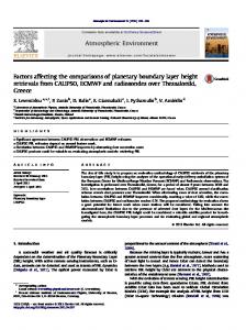
This section presents results of two trade-wind cumulus cases: one non-precipitating (BOMEX) and one precipitating (RICO). Figure 1 displays model sensitivity to 1t and 1z for both CAM-BASE and CAM-CLUBB for the BOMEX case of non-precipitating shallow cumulus. The top row shows the biases of integrated low cloud amount averaged over the last 2 h of the simulation for each CAM configuration. The LES value (C = 0.12) is denoted in the model configuration cell www.geosci-model-dev.net/5/1407/2012/


1411

Integrated Low Cloud Amount Bias


2400

LES 0.12 (fraction)

2400

0.6

2100

0.6

2100

LES 1200 0.12 (fraction)

0

900

−0.2

timestep (s)

600

0.2

1500 1200

0

900

−0.2

600 −0.4

−0.4

300

300 −0.6

60 30

60

90

120

150

180

210

−0.6

60

240

30

60

# of Vertical Levels

90

120

150

180

210

240


(a) CAM-BASE

(b) CAM-CLUBB

Liquid Water Path Bias

Liquid Water Path Bias 60

60

2400

2400

2100

40

2100

40

1800

1200

0

900 −20 600

1500 1200

0

900 −20

2

2

20

timestep (s)

20

LES 8 2 (g/m )

1500

SCM − LES (g/m )

timestep (s)

1800

SCM − LES (g/m )

timestep (s)

0.2

1500

1800

SCM − LES (fraction)

0.4 SCM − LES (fraction)

0.4 1800

600

300

−40

60

LES 300 8 2 (g/m )

−40

60 −60 30

60

90

120

150

180

210

240


(c) CAM-BASE

−60 30

60

90

120

150

180

210

240


(d) CAM-CLUBB

1: Biasesintegrated of vertically integrated low cloud b) and liquid path (c, SCAM-BASE d) from SCAM-BASE (a, c) and Fig. 1. Biases Fig. of vertically low cloud amount (a, amount b) and (a, liquid water pathwater (c, d) from (a, c) and SCAM-CLUBB (b, SCAM-CLUBB (b, d). Displayed is the BOMEX case of nonprecipitating trade-wind cumulus, averaged over hours 4–6 of the d). Displayed is the BOMEX case of non-precipitating trade-wind cumulus, averaged over hours 4–6 of the simulation. Plotted in each cell simulation. Plotted in each cell is the bias computed with respect to LES for a different value of ∆z and ∆t. The cell marked is the bias computed with respect to LES for awith different 1z the andLarge 1t. The marked(LES) “LES” the configuration “LES” indicates the configuration the bestvalue matchofwith Eddycell Simulation forindicates the particular variable. The with the best match with thevalue largeineddy simulation (LES) for the this box is the value computed by particular LES for thisvariable. regime. The value in this box is the value computed by LES for this regime.

that corresponds to the best match with LES. Light hues indicate a relatively small bias, whereas dark hues represent a large bias. White cells indicate near perfect agreement with LES. The BOMEX case is characterized by small cloud fraction, which is often difficult for moist parameterizations to simulate accurately due to the highly skewed nature of the cloud and turbulence properties of this regime. This is true for CAM-BASE, which tends to overestimate the integrated cloud fraction at most configurations of 1t and 1z, although the CAM-BASE bias is small at operational resolution. The overestimate becomes most pronounced when the number of levels and 1t increases. Similar sensitivities can also be found in the temporally averaged liquid water path (LWP) results (Fig. 1c) for CAM-BASE. CAM-CLUBB, on the other hand, shows a slight negative bias for both integrated cloud fraction and LWP. However, it shows much less sensitivity to changes in 1t and 1z, even for configurations with high vertical resolution and coarse time step, which is an encouraging result. Another experiment was performed in which the number of allowed iterations for the UWMT, UWSC, and Park


macrophysics were all set equal to the number of CLUBB sub-time steps for each respective host model time step. Results (not shown) looked nearly identical to those of Fig. 1. Increasing the number of iterations for CAM-BASE parameterizations for BOMEX at high vertical resolution and coarse time step smooths the mean time profiles, but otherwise does not much change the overall result. In addition, these SCAM-BASE simulations were more expensive than SCAM-CLUBB simulations for nearly all 1t configurations. Figure 2 displays the horizontally and temporally averaged profiles of cloud fraction and ql for simulations using 1t = 300 s, with 30 and 240 vertical levels. While this time step is much smaller than that traditionally used in GCMs, it is selected because CAM-BASE profiles are quite noisy for the operational time step when the vertical grid spacing is fine. For both simulation configurations, CAM-CLUBB properly represents cloud base and cloud top, and it reasonably simulates cloud amount and coverage. While cloud fraction suffers from a systematic negative bias near cloud base, ql simulated by CAM-CLUBB compares well with LES. As

Geosci. Model Dev., 5, 1407–1423, 2012

1412

P. A. Bogenschutz et al.: High-order turbulence closure for CAM Cloud Fraction

Cloud Liquid Water Mixing Ratio

700

750

800

750

pressure (hPa)

pressure (hPa)

700

LES CAM−BASE 30L CAM−BASE 240L CAM−CLUBB 30L CAM−CLUBB 240L

850

900

950

800

850

900

950

1000

1000

0

0.05

0.1

0.15

0.2

0.25

0.3

0

0.01

0.02

(fraction)

(a)

0.04

0.05

(b)

SGS Vertical Velocity

Cloud Number Concentration

700

700

750

750

800

800

pressure (hPa)

pressure (hPa)

0.03

(g/kg)

850

900

850 900 950

950

1000

1000 0

0.1

0.2

0.3

0.4

(m/s)

(c)

0

0.5

1

1.5

(#/m3)

2

2.5

3 7

x 10

(d)

Fig. 2: Temporally averaged profiles of cloud fraction, cloud liquid water mixing ratio, SGS vertical velocity, and droplet

Fig. 2. Temporally averaged profiles of cloud fraction, cloud liquid water mixing ratio, SGS vertical velocity, and droplet number concennumber concentration from hours 4–6 of the simulation for the BOMEX case of non-precipitating trade-wind cumulus. LES is tration fromdenoted hours 4–6 ofsolid the simulation for the BOMEX case of trade-wind cumulus. here LESare is denoted by with the solid black by the black line, and SCAM simulations arenon-precipitating denoted by the colored lines. Displayed simulations line, and SCAM simulations are denoted the colored lines. Displayed here are=simulations withNote 30 vertical (solid) and 240 vertical 30 vertical levels (solid) and 240by vertical levels (dashed), both using a ∆t 300s time step. that the levels minimum allowable −1 Note that the minimum allowable SGS vertical velocity in CAM is 0.2 m s−1 . levels (dashed), both using a 1tin=CAM 300 sistime step. SGS vertical velocity 0.2 ms .

suggested in Fig. 1, the robustness to changes in 1z for this case is remarkable. The simulated profiles of CAM-CLUBB appear to improve upon those simulated by CAM-BASE. While CAMBASE profiles of cloud fraction and ql are clearly representative of a trade-wind cumulus regime, both configurations of 1z suffer from cloud fraction that is too large and cloud layers that are too shallow. Note that cloud fraction profiles are substantially different than those presented in Park and Bretherton (2009). This is because that study presented only the cumulus cloud fraction and neglected the stratiform contribution. Here we show the shallow convective plus stratiform cloud. One possible reason CAM-CLUBB simulates better cloud depth is that the vertical velocity distribution near cloud top is highly skewed (not shown), as only a few clouds of this regime reach these heights. In CLUBB, w0 3 is simulated well and hence the cloud macrophysical quantities benefit. CAM-BASE appears to simulate only the numerous shallow clouds that occur near cloud base. It is also important to mention that about half of the cloud produced near Geosci. Model Dev., 5, 1407–1423, 2012

cloud base in CAM-BASE is from the UWMT scheme. As BOMEX is a purely trade-wind cumulus regime, one would expect the cloud to be represented solely by a shallow convection scheme. Since CLUBB is a unified parameterization of PBL and shallow convection that produces all cloud, this counter-intuitive behavior is avoided. CAM-CLUBB’s SGS vertical velocity profile (Fig. 2c) is improved when compared to CAM-BASE in both the sub-cloud mixed layer (roughly below 950 hPa) and in the cloud layer. The SGS vertical velocity in the cloud layer for CAM-BASE defaults to the minimum allowable value of 0.2 m s−1 for nearly all choices of 1z, suggesting that the UWSC scheme dominates at these levels, as one would expect. Therefore, the separate microphysics scheme within the UWSC parameterization is active in the cumulus layers. In contrast, since CAM-CLUBB utilizes the MG microphysics scheme for shallow cumulus as well as stratiform cloud, CAM-CLUBB’s representation of w0 and MG microphysics are available to activate aerosol and predict droplet concentration in a unified manner. www.geosci-model-dev.net/5/1407/2012/

Bogenschutz et al.: High Order Turbulence Closure for CAM

13


1413

Surface Precip. Rate Bias

Surface Precip. Rate Bias 1

LES 0.558 (mm/day)

0.8

2100

0.8 2100

1500

0.2

1200

0 −0.2

900

−0.4

600

0.4

1500

0.2

1200

0 −0.2

900

−0.4

600

−0.6

300

0.6

1800

timestep (s)

0.4

SCM − LES (mm/day)

0.6

1800

timestep (s)

1 2400

LES 0.558 (mm/day)

300

−0.8 60


2400

−0.6 −0.8

60 −1 30

60

90

120

150

180

210

−1

240

30


60

90

120

150

180

210

240


(a) CAM-BASE

(b) CAM-CLUBB

Fig. 3: Same as Fig. 1, except for the bias of surface precipitation rates from the RICO case of precipitating trade-wind

Fig. 3. Same ascumulus, Fig. 1, averaged except for thehours bias18–24. of surface precipitation rates from the RICO case of precipitating trade-wind cumulus, averaged over over hours 18–24.

2

(g/m )

(−)

The above presentation demonstrates that CAM-CLUBB similar behavior to that of Fig. 1 for both CAM-BASE and produces reasonable results for the challenging regime of CAM-CLUBB and is therefore not displayed here. non-precipitating trade-wind cumulus clouds. The precipiCAM-CLUBB captures the timing of the onset/decay of tating trade-wind cumulus case (RICO) was also performed cumulus clouds in response to surface forcing fairly accuwith CAM-BASE and CAM-CLUBB. We found similar rately (Fig. 4). While cumulus initiation and decay are both Water Pathcloud fraction is underestimated, quality results for cloud fraction, ql , w 0 ,Cloud and Cover Nd (cloud numdelayed and theCloud integrated 0.5 100 LES ber concentration) as displayed in the BOMEX case (not the CAM-CLUBB configuration shows improvement when 0.45 90 CAM−BASE 30 L shown). Figure 3 illustrates both CAM-BASE and CAMcompared to CAM-BASE. CAM-BASE tends to predict too CAM−CLUBB 30 L 0.4 80 CLUBB’s ability in representing the light precipitation rates much fog early in the simulation and fails to dissipate the 0.35 70 observed in this case for all combinations of 1z and 1t. clouds near the end of the simulation in response to declin0.3 60 CAM-BASE has a tendency to overpredict the amount of ing surface fluxes. 0.25 50 rain that reaches the surface for this drizzling cumulus case 0.2 40Overall, it appears that CAM-CLUBB can treat shallow for nearly all configurations of 1z and 1t. Oftentimes this cumulus (both maritime and continental) with fidelity. This 0.15 30 overestimation reaches 0.1 a factor of three or four and is likely is20an encouraging result, as many recent studies (Gettelman 0.05tendency to overpredict the liquid due to the CAM-BASE et10al., 2012; Medeiros et al., 2008) suggest that shallow cu0 water and cloud amount.0Most of the precipitation produced mulus convection contributes more strongly than stratocumu0 0.1 0.2 0.3 0.4 0.5 0.6 0 0.1 0.2 0.3 0.4 0.5 0.6 time (day) time (day) for CAM-BASE comes from the shallow convection milus clouds to climate feedbacks and sensitivity, due partly crophysics scheme. CAM-CLUBB’s are more robust to the of the covered bycase shallow cumulus. Fig. 4: Temporal evolution ofresults the integrated low cloud fraction and liquidlarge waterarea path from the globe simulations of ARM of across the 1t continental and 1z spectrum and in better agreement with However, while maritime stratocumulus clouds cover a much shallow cumulus with 30 vertical levels and a 60-s time step. surface precipitation computed from the LES. The higher smaller portion of the global ocean, they are significant modprecipitation rates could also be a reason for the excessive ulators of the Earth’s radiation budget and increase the overshallowness of simulated cumulus layers in CAM-BASE. all albedo (Hartmann et al., 1992) and must also be properly represented in GCMs. Therefore, the next test is to examine stratocumulus and transitional regimes. 3.2 Continental cumulus 3.3 The continental cumulus case that we investigate was observed over the ARM site in Oklahoma (Brown et al., 2002). The ARM case is qualitatively different than the maritime shallow cumulus case in that the ARM clouds are diurnally driven by time varying surface sensible heat fluxes, surface latent heat fluxes, and large-scale forcings as opposed to the quasi steady state reached in the BOMEX and RICO cases. Therefore, the ARM case allows us to test the timing of onset and decay of convection, in which clouds form over an initially clear convective boundary layer. The representation of C and ql to changes in 1z and 1t for the ARM case exhibits www.geosci-model-dev.net/5/1407/2012/

Cumulus under stratocumulus

Transitional regimes are typically found downwind of classical maritime stratocumulus regimes and consist of tradewind cumulus underneath broken stratocumulus. Hence, this regime combines qualitative properties of both cumulus (i.e. BOMEX or RICO) as well as stratocumulus (i.e. DYCOMS2-RF01). It is important that any physics parameterization be able to represent this type of regime in order to achieve realistic global distributions of shortwave cloud forcing. We use the ATEX case as a benchmark for the stratocumulus over cumulus regime, which was studied in the LES Geosci. Model Dev., 5, 1407–1423, 2012

1414

P. A. Bogenschutz et al.: High-order turbulence closure for CAM Cloud Water Path 100

0.45

90

0.4

80

0.35

70

0.3

60

0.25 0.2

14

LES CAM−BASE 30 L CAM−CLUBB 30 L

2

(g/m )

(−)

Cloud Cover 0.5

50 40

30 Bogenschutz et al.: High Order Turbulence Closure for CAM

0.15 0.1

20

0.05

10

0

0

0

0.1

0.2

0.3

0.4

0.5

0.6

0

0.1

0.2

0.3

0.4

0.5

0.6

time (day)

time (day)

Fig. 4: Temporal evolution of the integrated low cloud fraction and liquid water path from the simulations of ARM case of

Fig. 4. Temporal evolution of the integrated low cloud fraction and liquid water path from the simulations of ARM case of continental continental shallow cumulus with 30 vertical levels and a 60-s time step. shallow cumulus with 30 vertical levels and a 60-s time step.



2400

0.6 LES 0.42 (fraction)

0.4

1200

0

900

−0.2

timestep (s)

600

0.2

1500 1200

0

900

−0.2

600 −0.4

−0.4

300

300 −0.6

60 30

60

90

120

150

180

210

−0.6

60

240

30

60


90

120

150

180

210

240


(a) CAM-BASE

(b) CAM-CLUBB



2400 2100

40

60

LES 20 2 (g/m )

2400 2100

40

1800

1200

0

900 −20 600

1500 1200

0

900 −20

2

2

20

timestep (s)

20 1500

SCM − LES (g/m )

1800

SCM − LES (g/m )

timestep (s)

0.2

1500

1800


0.4

1800

timestep (s)

0.6

2100


2100

LES 0.42 (fraction)

2400

600 LES 20 2 (g/m )

300

−40

60

300

−40

60 −60 30

60

90

120

150

180

210

240


(c) CAM-BASE

−60 30

60

90

120

150

180

210

240


(d) CAM-CLUBB

as Fig. 1 except averaged over hours 4–8 of the simulation for the ATEX case of cumulus under stratocumulus. Fig. 5. Same asFig. Fig.5:1Same except averaged over hours 4–8 of the simulation for the ATEX case of cumulus under stratocumulus.

intercomparison of Stevens et al. (2001). Each different LES in that study was able to capture the general characteristics of this regime; however, cloud amounts at inversion top varied greatly between codes (with vertically integrated cloud fractions ranging from 0.2 to 0.8). Figure 5 displays the biases of CAM-BASE and CAMCLUBB for the integrated cloud amount and LWP for the

Geosci. Model Dev., 5, 1407–1423, 2012

ATEX simulation for hours 4–8 of the simulation. Integrated cloud fraction amounts for CAM-CLUBB are clearly more sensitive for this case than they were for the shallow cumulus cases, with values ranging from 0.25 to 0.98, depending on the simulation configuration and with less of a discernible pattern. However, CAM-CLUBB tends to have more instances where the integrated cloud fraction and LWP match


Bogenschutz et al.: High Order Turbulence Closure for CAM

15


1415

Surface Precip. Rate Bias

Surface Precip. Rate Bias 1

1

2400

2400 0.8

1500

0.2 LES 0 (mm/day)

1200

0 −0.2

900

−0.4

600

−0.6

300

0.6

1800

timestep (s)

0.4


timestep (s)

1800

16

0.8 2100

0.6

0.4

1500

0.2

1200

0 LES 0 (mm/day)

900

−0.2 −0.4

600


2100

Bogenschutz et al.: High Order Turbulence Closure −0.6 for CAM 300

−0.8

−0.8

60

60 −1 30

60

90

120

150

180

210

−1

240

30

60

90


120

150

180

210

240


(a) CAM-BASE

(b) CAM-CLUBB

6: Same as Fig. 1, except for the bias of surface precipitation rates from the ATEX case of cumulus under stratocumulus, Fig. 6. Same asFig. Fig. 1, except for the bias of surface precipitation rates from the ATEX case of cumulus under stratocumulus, averaged over averaged over hours 4–8. hours 4–8.

Cloud Fraction


700

750

750

Table 1: Summary of cases used for800 single-column CAM testing

800

Cases

Full Name

DYCOMS2-RF01


850

900

950

DYCOMS2-RF02


1000 0

0.1

0.2

ATEX

0.3

0.4

(fraction)

(a)

0.5

0.6

pressure (hPa)

pressure (hPa)

700


0.7

0.02

0.04

0.06

0.08

0.1

0.12

0.14

(g/kg)

Stevens et al. (2001) (b)


850

ARM

Ackerman et al. (2009)

Maritime cumulus under stratocumulus

Rain in Cumulus Over Ocean Atmospheric Radiation Measurement

900

900

0

Atlantic Trade Wind Experiment

700 Marine shallow cumulus

Siebesma et al. (2003)

750

pressure (hPa)

pressure (hPa)

RICO

800


drizzling 1000 stratocumulus

Barbados Oceanographic and Meteorological Experiment

750

References


950 Maritime


BOMEX

700

Regime Type

850

Precipitating 800

Rauber et al. (2003)

marine shallow cumulus 850 Continental 900 shallow cumulus

Brown et al. (2002)

950

950

1000

1000 0

0.1

0.2

0.3

0.4

(m/s)

(c)

0.5

0

1

2

(#/m3)

3

4 7

x 10

(d)

Fig. 7: Same as Fig. 2 except SCAM profiles represent ATEX simulations averaged over hours 4–8, with fixed ∆t = 300s and

Fig. 7. Same as30Fig. except SCAM and 2240 vertical levels. profiles represent ATEX simulations averaged over hours 4–8, with fixed 1t = 300 s and 30 and 240 vertical levels.

LES (0.42 and 20 g m−2 ), indicated by a clear or lightly hued cell, when compared to CAM-BASE. There are several instances where LWP and integrated cloud fraction resemble a purely stratocumulus (Sc) regime for CAM-BASE, and a few instances of this for CAM-CLUBB. For CAMCLUBB it appears that this sensitivity is ameliorated for con-


figurations using high vertical resolution, suggesting that this particular regime requires fine vertical grid spacing, as one would expect. Meanwhile, simulated LWP and integrated cloud fraction tend to degrade as vertical resolution becomes finer at longer time steps in the CAM-BASE configuration.

Geosci. Model Dev., 5, 1407–1423, 2012

1416

P. A. Bogenschutz et al.: High-order turbulence closure for CAM Integrated Low Cloud Amount Bias

Integrated Low Cloud Amount Bias 0.2

0.2

2400

2400 0.15

0.15 2100

1500

0.05

1200

0

900

−0.05 LES 0.987 (fraction)

600

0.1

1800

timestep (s)

1500

0.05

1200

0

900

−0.05

600

−0.1

300

−0.1

300 −0.15

60 30

60

90

120

150

180

210

240

30

60


120

150

180

−0.2

210

240

(b) CAM-CLUBB



LES 38.2 2 (g/m )

60 2400

2100

40

2100

40

1800

1200

0

900 −20 600

1500 1200

0

900 −20

2

2

20

timestep (s)

20 1500

SCM − LES (g/m )

1800

timestep (s)

90


(a) CAM-BASE

2400

−0.15

LES 0.987 (fraction)

60 −0.2

SCM − LES (g/m )

timestep (s)

1800


0.1


2100

600

300

−40

60

LES 38.2 2 (g/m )

300

−40

60 −60 30

60

90

120

150

180

210

−60

240

30


60

90

120

150

180

210

240


(c) CAM-BASE

(d) CAM-CLUBB

Fig. 8: Same as Fig. 1 except averaged over hours 4–6 of the simulation for the DYCOMS2-RF01 case of maritime stratocu-

Fig. 8. Same as Fig. 1 except averaged over hours 4–6 of the simulation for the DYCOMS2-RF01 case of maritime stratocumulus. mulus.

It is important to note that ATEX is an observationally non-precipitating case, although in these simulations we keep the microphysics turned on and allow precipitation in order to obtain a less idealized and more realistic simulation. For 94 % of the simulations, CAM-CLUBB (Fig. 6) correctly predicts a zero surface precipitation rate whereas CAM-BASE produces large biases with precipitation rates of 0.4 mm day−1 or higher (up to 2 mm day−1 ) for 70 % of the simulations. It appears that the majority of this precipitation is generated by the UWSC scheme. Figure 7 displays the temporally averaged profiles of C and ql for CAM-BASE and CAM-CLUBB between hours 4–8 of the ATEX case for 30 and 240 levels and fixed 1t = 300 s. This figure shows that both configurations of CAMCLUBB are able to realistically represent the basic structure of the cumulus under stratocumulus regime. Although cloud top C and ql are underestimated for the 30-level case, both CAM-CLUBB curves are within the range of the LES ensemble of Stevens et al. (2001). In addition, CAM-CLUBB profiles appear to be more realistic than CAM-BASE profiles, which tend to place the vertical maximums of C and ql in the levels where cumulus, rather than stratocumulus, should be prevalent. This overrepresentation occurs because both the UWSC and UWMT schemes are active near cloud base. However, near Sc cloud top, nearly all cloud is produced from the Park stratiform macrophysics, as one would

Geosci. Model Dev., 5, 1407–1423, 2012

expect. Similar to results from BOMEX, CAM-CLUBB has a good representation of w0 throughout the boundary layer; however, CAM-BASE underestimates w 0 throughout the entire cloud layer. 3.4


The last regime we examine is a maritime stratocumulus regime, namely the DYCOMS2-RF01 (hereafter RF01) and DYCOMS2-RF02 (hereafter RF02) cases. RF01 is challenging case in which the stratocumulus cloud deck was observed to persist despite classical theories that suggested it should have dissipated over time (i.e. Randall, 1980). RF02 is a marine Sc case that was observed to contain drizzle (Ackerman et al., 2009). The standard GCSS case setup for RF01 (Stevens et al., 2005) is a 6-h nocturnal simulation with prescribed and constant surface and latent heat fluxes. The setup we use is identical to that described in Stevens et al. (2005), except that we extend the case to four days with a diurnal cycle in radiative forcing. The GCSS averaging interval is still examined for direct comparison with LES for CAM-BASE and CAM-CLUBB. However, we expect the marine Sc to persist through the four-day period. First we examine the sensitivity of CAM-BASE and CAM-CLUBB to 1z and 1t for the GCSS averaging interval of hours 4–6 of the simulation. Figure 8 displays the biases in integrated low cloud amount (top row) and www.geosci-model-dev.net/5/1407/2012/



850

850

LES CAM−BASE 30L CAM−BASE 60L CAM−CLUBB 30L CAM−CLUBB 60L 900

pressure (hPa)

pressure (hPa)

1417

950

1000

900

950

1000

0

0.2

0.4

0.6

0.8

1

0

0.1

(fraction)

(a)

0.3

0.4

(b) Cloud Number Concentration

SGS Vertical Velocity 850

850

900

900

pressure (hPa)

pressure (hPa)

0.2

(g/kg)

950

950

1000

1000 0

0.1

0.2

0.3

0.4

0.5

0.6

(m/s)

(c)

0.7

0

2

4

(#/m3)

6

8 7

x 10

(d)

Fig.as9:Fig. Same as Fig.SCAM 2 exceptprofiles SCAMrepresent profiles represent DYCOMS2-RF01 simulations averaged over hours 4–6, fixed with fixed 3060 vertical Fig. 9. Same 2 except DYCOMS2-RF01 simulations averaged over hours 4–6, with 30 and and 60 vertical levels and ∆t = 1800s. levels and 1t = 1800 s.

LWP (bottom row). Unlike the results for the convective cumulus cases, results between the two model configurations do not differ greatly. This is in agreement with Bretherton and Park (2009), who showed that the UWMT scheme is robust to changes in 1z for marine stratocumulus. LES suggests an integrated low cloud amount ∼ 1, and it appears that both CAM configurations can produce solid cloud cover for most 1z and 1t configurations. The largest (negative) biases for both CAM-BASE and CAM-CLUBB occur for the operational 30-level configurations. Upon examination of the LWP, it is evident that almost all simulation configurations overestimate this quantity. This is surprising since one might expect parameterizations to underestimate cloud water for RF01 due to the very dry air in the free troposphere. However, this positive bias appears to be due to the tendency of both CAM-BASE and CLUBB parameterizations to produce cloud layers that are slightly too thick compared to LES, which is consistent with the findings of Zhu et al. (2005). However, bias patterns and magnitudes are similar for CAMBASE and CAM-CLUBB.


Temporally averaged profiles of CAM-BASE and CAMCLUBB can be viewed in Fig. 9 over the GCSS averaging interval. In this figure the configurations use the operational time step of 1t = 1800 s for 30 and 60 levels. While CAMCLUBB predicts less cloud coverage for the operational 30 grid level when compared to CAM-BASE, the levels of cloud base and cloud top are better represented for CAM-CLUBB for both 1z configurations. For the case of 60 vertical levels, CAM-CLUBB has better agreement with LES for C and ql , both in terms of vertical placement and magnitude. While it is evident that CAM-CLUBB is more sensitive to changes in 1z for this case, the improvement for the 60 level case over CAM-BASE is encouraging. In terms of SGS vertical velocity, CAM-CLUBB underestimates w 0 for the 30-level case. This occurs probably because there is a lack of cloud cover and mass compared to LES, which acts to reduce cloud-top feedbacks that are necessary to maintain an adequately turbulent mixed layer. Along with SGS vertical velocity, accurate representation of Nd is also required to represent aerosol indirect effects. In both simulations Nd is predicted by the MG microphysics

Geosci. Model Dev., 5, 1407–1423, 2012

1418

P. A. Bogenschutz et al.: High-order turbulence closure for CAM Cloud Liquid Water Mixing Ratio

Cloud Liquid Water Mixing Ratio 0.4

0.4

860

860 0.35

0.35

880

880

0.25

920

0.2

940

0.15

960

0.1

0.05

980

0.3

pressure (hPa)

pressure (hPa)

0.3

900

900

0.25

920

0.2

940

0.15

960

0.1

0.05

980

0

0

1

2

3

4

time (day)

0

0

1

2

3

4

time (day)

(a) CAM-BASE

(b) CAM-CLUBB

(c) CAM-BASE

(d) CAM-CLUBB

−1 Fig. 10: Evolution of the cloudwater liquidmixing water ratio mixing ratio ) for CAM-BASE (a, CAM-CLUBB c) and CAM-CLUBB (b, d) the foursimulation −1(gkg Fig. 10. Evolution of the cloud liquid (g kg ) for CAM-BASE (a, c) and (b, d) for thefor four-day day simulation of DYCOMS2-RF01 using 30 vertical levels and ∆t = 1800s (a, b) and 240 vertical levels and ∆t = 60s. of DYCOMS2-RF01 using 30 vertical levels and 1t = 1800 s (a, b) and 240 vertical levels and 1t = 60 s (c, d).

scheme, and both CAM-BASE and CAM-CLUBB simulations can adequately represent this quantity. However, CAMCLUBB underestimates Nd using 30 levels, due to the underestimation of cloud mass as well as w0 . Overall, the simulations of RF01 for both CAM-BASE and CAM-CLUBB do not vary greatly during the GCSS averaging interval. Next we test whether either configuration can maintain the cloud through the entire four-day period, including the daytime periods when the cloud is expected to thin due to incoming shortwave radiation and decouple from the wellmixed layer below (Krueger et al., 1995). The cloud deck is expected to regain its optical thickness during the nighttime when longwave radiational cooling at cloud top becomes the dominate source of turbulence. This can be thought of as a more “real world” test for GCM parameterization. Figure 10 displays the evolution of the cloud water mixing ratio for both CAM-BASE and CAM-CLUBB for the entire four-day simulation. We test an operational configuration with 30 levels and 1t = 1800 s (top row) and a high-resolution configuration with 240 levels and 1t = 60 s. For both configurations, CAM-BASE tends to dissipate the cloud, gradually for the coarse-resolution simulation and Geosci. Model Dev., 5, 1407–1423, 2012

abruptly for the high-resolution simulation. Upon investigation, it appears that, during the day time period, once decoupling of the boundary layer occurs, the UWSC takes over the UWMT scheme and the Sc deck undergoes a transition to a more cumulus-like state. This is consistent with forecasts of stratocumulus in Medeiros et al. (2012). CAM-CLUBB, on the other hand, maintains the cloud in both configurations for the entire four day period, with a diurnal cycle present in both grid simulations. Note that the strong oscillations for both CAM-BASE and CAM-CLUBB in the 30-level configuration appear to be related to the rather coarse time step as these oscillations do not appear in the 30-level configuration with 1t = 60 s (not shown). The second marine Sc case we investigate is the RF02 case, which is set up in SCAM exactly as described in Ackerman et al. (2009). This case is often thought to be easier to simulate than RF01 because the inversion for both temperature and moisture is not quite as sharp above cloud top. Indeed, intercomparison agreement among LES is better for RF02 (Ackerman et al., 2009) than for RF01 (Stevens et al., 2005). Unlike the RF01 case, we only simulate this case over the 6-h GCSS interval. www.geosci-model-dev.net/5/1407/2012/


1419


Integrated Low Cloud Amount Bias 0.1

0.1

2400

2400 0.08

1500

0.02 LES 0.996 (fraction)

1200

0 −0.02

900

−0.04

600

0.04

1500

0.02

1200

0 −0.02

900

−0.04

600

−0.06

300

0.06

1800

timestep (s)

0.04


1800

LES 0.996 (fraction)

300

−0.08 60

−0.06 −0.08

60 −0.1 30

60

90

120

150

180

210

−0.1

240

30

60


90

120

150

180

210

240


(a) CAM-BASE

(b) CAM-CLUBB



60 2400

2100

40

2100 1800

1200

0

900 −20 600

2

timestep (s)

timestep (s)

20 1500

SCM − LES (g/m )

1800

40 LES 107 2 (g/m )

20

1500 1200

0

900 −20

2

2400

SCM − LES (g/m )

timestep (s)

0.08 2100

0.06


2100

600 LES 107 2 (g/m )

300

−40

60

300

−40

60 −60 30

60

90

120

150

180

210

240


(c) CAM-BASE

−60 30

60

90

120

150

180

210

240


(d) CAM-CLUBB

Fig. 11:1Same as Fig. 1 except averaged of the simulation the DYCOMS2-RF02 maritimestratocumulus. stratocuFig. 11. Same as Fig. except averaged over hoursover 4–6hours of the4–6 simulation for thefor DYCOMS2-RF02 casecase of of maritime mulus.

While CAM-CLUBB’s sensitivity of integrated cloud fraction to changes in 1z and 1t is decidedly more robust for RF02 compared to RF01 (Fig. 11), LWP has more variation for both model configurations. This is somewhat surprising and suggests that the CAM microphysics scheme could be playing more of a role here than in the non-precipitating RF01 case. Whereas LES suggests a LWP of 107 g m−2 , more often than not CAM-BASE and CAM-CLUBB either underestimate or overestimate this value. However, the minimum LWP values by both model configurations (∼ 60 g m−2 ) are still representative of a marine stratocumulus regime. It should be noted that, for both RF01 and RF02, the sensitivities of surface precipitation rates to 1t and 1z are nearly identical for CAM-BASE and CAM-CLUBB. Therefore, an analogous plot to Fig. 3 is not shown for these cases. Figure 12 displays the temporally averaged profiles over hours 4–6 of cloud fraction, ql , w 0 , and Nd for CAM-BASE and CAM-CLUBB for the DYCOMS2-RF02 case. The time step in these profiles is fixed to 1t = 300 s with the 30 and 240 vertical levels. In terms of C and ql , there is very little difference seen between CAM-BASE and CAM-CLUBB. Overall, the differences seen in the stratocumulus cases (RF01 and RF02) between CAM-BASE and CAMCLUBB are smaller than the differences seen in cumulus


cases or transitional ATEX case. This is especially clear when evaluating the GCSS averaging intervals for nocturnal stratocumulus. However, when a diurnal cycle is considered, it appears that CAM-CLUBB can maintain the cloud deck through the simulation more successfully than CAM-BASE, owing to interactions between the separate turbulence and shallow convection schemes. 4 Conclusions This paper describes the coupling of CAM with a relatively new parameterization, CLUBB. CLUBB is a higherorder turbulence closure based upon an assumed doubleGaussian probability density function (PDF). The assumed PDF is used to compute many unclosed turbulent moments and cloud macrophysical quantities, such as cloud fraction and cloud water mixing ratio. This “unified” closure is inherently different than traditional parameterizations used in GCMs as it is responsible for providing the tendencies of turbulent mixing from the PBL, shallow convection, and cloud macrophysics in one parameterization call rather than splitting these duties among several different parameterizations that may or may not be consistent with one another. In addition, CLUBB drives a single microphysics scheme (MG) for Geosci. Model Dev., 5, 1407–1423, 2012

1420



850

850

900

pressure (hPa)

pressure (hPa)


950

1000

900

950

1000

0

0.2

0.4

0.6

0.8

1

0

0.1

0.2

0.3

(fraction)

(a)

0.5

0.6

0.7

(b)



850

850

900

900

pressure (hPa)

pressure (hPa)

0.4

(g/kg)

950

950

1000

1000 0

0.2

0.4

0.6

0.8

(m/s)

(c)

1

0

2

4

6

(#/m3)

8

10

12 7 x 10

(d)

Fig. 12: Same as Fig. 2 except SCAM profiles represent DYCOMS2-RF02 simulations averaged over hours 4–6, with fixed 30

Fig. 12. Same as Fig. 2 except SCAM and 240 vertical levels and ∆t =profiles 300s. represent DYCOMS2-RF02 simulations averaged over hours 4–6, with fixed 30 and 240 vertical levels and 1t = 300 s.

both shallow convection and stratiform cloud, whereas the shallow convection scheme in CAM-BASE has its own treatment of microphysics. Therefore, CLUBB allows for a more unified treatment of cloud-aerosol interactions. For the coupling of CAM with CLUBB described in this paper, CLUBB replaces the University of Washington Moist Turbulence (UWMT, Bretherton et al., 2009) scheme, the University of Washington Shallow Convection (UWSC; Park and Bretherton, 2009) scheme, and the cloud macrophysics scheme in CAM5. The physics that are retained in CAMCLUBB include the deep convection (Zhang and McFarlane, 1995; Neale et al., 2008; Richter and Rasch, 2008), aerosol (Liu et al., 2011) and microphysics schemes (Morrison and Gettelman, 2008). In the CAM-CLUBB configuration, the SGS vertical velocity (w 0 ) is computed from the predicted w0 2 and is passed to the aerosol activation scheme. Results from single-column CAM (SCAM) testing were presented in this paper for a wide range of boundary layer regimes. These include shallow cumulus, transitional regimes, as well as maritime stratocumulus regimes. To test the robustness of the models, a direct comparison between

Geosci. Model Dev., 5, 1407–1423, 2012

CAM-BASE and CAM-CLUBB is performed for a variety of temporal and vertical resolutions, with the main model time step, 1t, varying from 60 s to 2400 s and 1z varying from configurations utilizing 30 levels to 240 levels. The operational configuration of CAM consists of 1t = 1800 s and 30 vertical levels. It is important to note that, in this study, CLUBB is subcycled with a time step of 5 min, whereas CAM-BASE’s cloud parameterizations are not subcycled but rather use the full model time step of 1800 s. However, using CLUBB with a time step of 300 s increases the overall computational cost by only 4 % relative to the standard configuration of CAM-BASE, in which a time step of 1800 s is used for all parameterizations. CLUBB’s subcycled time step is analogous to the iteration loops in the CAM-BASE physics options that are shut off in CAM-CLUBB. Furthermore, experiments suggest that increasing the number of iteration cycles for CAM-BASE parameterizations does not necessarily lead to better results at coarse host model time steps. For cases of shallow cumulus convection (i.e. BOMEX, RICO, and ARM), it appears that CAM-CLUBB has advantages compared to CAM-BASE. For all shallow cumulus


P. A. Bogenschutz et al.: High-order turbulence closure for CAM cases that we tested, CAM-CLUBB is more robust to changes in 1t and 1z while providing results that are in better agreement with LES. CAM-BASE tends to produce cumulus layers that are too shallow and cloudy, likely due to limitations of the mass flux scheme to represent the highly skewed vertical velocity statistics of this regime. In contrast, CAM-CLUBB predicts w0 3 and hence vertical velocity skewness, which allows for more accurate representation of this regime, with SGS vertical velocity values in the cloud layer that highly resemble those from LES. In addition, surface precipitation rate for CAM-CLUBB, which relies on the MG microphysics for this regime, is in better agreement with LES and observations for the RICO case. In the CAM-BASE simulations, the UWMT moist turbulence scheme is responsible for contributing to the overly cloudy layers in the shallow cumulus regime. Because CLUBB is a unified parameterization of shallow cumulus and the PBL, it avoids the problem of the stratiform scheme contributing undesirably to cumulus simulations. CAM-CLUBB also has the ability to represent a realistic cumulus under stratocumulus boundary layer, as shown by comparisons to LES in the ATEX case. This result is especially encouraging as Kay et al. (2012) show negative low cloud biases for CAM4 and CAM5 in tropical transition regions. Results from the GCSS DYCOMS2-RF01 (RF01) and DYCOMS2-RF02 (RF02) cases of stratocumulus show fewer differences between CAM-BASE and CAM-CLUBB compared to the shallow cumulus cases. However, it is important to note that running RF01 for four days with a diurnal cycle shows that CAM-CLUBB can maintain the stratocumulus cloud better through this period compared to CAMBASE for most 1t and 1z configurations. During the latter days of the four-day RF01 simulation for CAM-BASE, the shallow convective scheme becomes active during the daytime hours, which more often than not leads to entrainment rates that are too high and an excessive depletion of liquid water. The results from these cases suggest that the configuration of CAM using CLUBB is more unified in the sense that it can represent both shallow cumulus and marine Sc with good agreement with LES. In addition, the results suggest promise for representation of indirect aerosol effects because CAM-CLUBB represents the SGS vertical velocity and cloud droplet concentration with fidelity. In addition, CAM-CLUBB employs the MG microphysics scheme for both shallow cumulus and stratocumulus, whereas CAMBASE uses separate microphysics schemes for these two regimes. Using a single microphysics scheme allows for a more consistent treatment of microphysics and aerosol interactions. The robustness of CAM-CLUBB, as well as the ability to use the same microphysics scheme for all of the cases tested, is encouraging. The results from the tradecumulus cases are especially encouraging as recent studies (Gettelman et al., 2012; Mederios et al., 2008) find that


1421

shallow cumulus regimes, with their widespread coverage across the globe, contribute most strongly to climate sensitivity and feedbacks. Although these single-column results are promising, the key test will involve running CAM-CLUBB globally. The hope is that the same caliber results found in these singlecolumn simulations will transfer over to multi-year and decadal global simulations. For this study, none of the tunable parameters within CLUBB were modified. However, tuning may become necessary in global simulations in order to achieve radiative balance or realistic distributions of cloud radiation forcing, for example. Future work will involve investigating the aerosol indirect effect, climate sensitivity, and feedbacks of CAM-CLUBB as compared to CAMBASE as well as other GCMs. One can take advantage of the SGS variability provided by CLUBB to generate subcolumns (Pincus et al., 2006) and thereby avoid the use of “maximum-random” cloud overlap assumptions in both microphysics and radiation parameterizations. In addition, as mentioned throughout this paper, one can take advantage of CLUBB’s SGS PDF information for treatment of microphysics and aerosol processes. For example, one can use the variance of liquid water and covariance of liquid water and rain water for computation of autoconversion and accretion process rates. In addition, we can integrate over the PDF for vertical velocity for the computation of aerosol activation (Ghan et al., 1997). These treatments will be explored in future versions of CAM-CLUBB. Acknowledgements. P. A. Bogenschutz is supported by National Science Foundation grant number 0968657. The National Center for Atmospheric Research is sponsored by the United States National Science Foundation. The authors are grateful to Brian Medeiros, Jennifer E. Kay, Steven J. Ghan, and an anonymous reviewer for reading and suggesting improvements to this manuscript. Edited by: H. Garny

References Ackerman, A. S., VanZanten, M. C., Stevens, B., Savic-Jovcic, V., Bretherton, C. S., Chlond, A., Golaz, J.-C., Jiang, H., Khairoutdinov, M., Krueger, S. K., Lewellen, D. C., Lock, A., Moeng, C.-H., Nakamura, K., Petters, M. D., Snider, J. R., Weinbrecht, S., and Zulauf, M.: Large-eddy simulations of a drizzling, stratocumulus-topped marine boundary layer, Mon. Weather Rev., 137, 1083–1110, 2009. Bogenschutz, P. and Krueger, S. K.: Improved boundary layer cloud simulations in cloud resolving models with a simple turbulence closure, submitted, 2012. Bogenschutz, P., Krueger, S. K., and Khairoutdinov, M.: Assumed probability density functions fo shallow and deep convection, J. Adv. Model. Earth Syst., 2, 10, doi:10.3894/JAMES.2010.2.10, 2010. Bony, S. and Dufresne, J.-L.: Marine boundary layer clouds at the heart of tropical cloud feedback uncertainties in climate model,

Geosci. Model Dev., 5, 1407–1423, 2012

1422


Geophys. Res. Lett., 32, L20806, doi:10.1029/2005GL023851, 2005. Bretherton, C. S. and Park, S.: A new moist turbulence parameterization in the community atmosphere model, J. Climate, 22, 3422–3448, 2009. Brown, A. R., Cederwall, R. T., Chlond, A., Duynkerke, P. G., Golaz, J.-C., Khairoutdinov, M., Lewellen, D. C., Lock, A. P., Macvean, M. K., Moeng, C.-H., Neggers, R. A. J., Siebesma, A. P., and Stevens, B.: Large-eddy simulation of the diurnal cycle of shallow cumulus convection over land, Q. J. R. Meteorol. Soc., 128, 1075–1094, 2002. Cheng, A. and Xu, K.-M.: Simulation of shallow cumuli and their transition to deep convective clouds by cloud-resolving models with different third-order turbulence closures, Q. J. R. Meteorol. Soc. doi:10.1256/qj.05.29, 2006. Cheng, A. and Xu, K.-M.: Improved low-cloud simulation from a multiscale modeling framework with a third-order turbulence closure in its cloud resolving model component, J. Geophys. Res., 115, D14101, doi:10.1029/2010JD015362, 2011. Donner, L. J., Wyman, B. L., Hemler, R. S, Horowitz, L. W., Ming, Y., Zhao, M., Golaz, J.-C., Ginoux, P., Lin, S.-J., Schwarzkopf, M. D., Austin, J., Alaka, G., Cooke, W. F., Delworth, T. L., Freidenreich, S. M., Gordon, C. T., Griffies, S. M., Held, I. M., Hurlin, W. J., Klein, S. A., Knutson, T. R., Langenhorst, A. R., Lee, H. C., Lin, Y., Magi, B. I., Malyshev, S. L., Milly, P. C. D., Naik, V., Nath, M. J., Pincus, R., Ploshay, J. J., Ramaswamy, V., Seman, C. J., Shevliakova, E., Sirutis, J. J., Stern, W. F., Stouffer, R. J., Wilson R. J., Winton, M., Wittenberg, A. T., and Zeng, F: The dynamical core, physical parameterizations, and basic simulation characteristics of the atmospheric component AM3 of the GFDL Global Coupled Model CM3, J. Climate, 24, 3484–3519, 2011. Gettelman, A., Liu, X., Ghan, S. J., Morrison, H., Park, S., Conley, A. J., Klein, S. A., Boyle, J., Mitchell, D. L., and Li, J.-L. F.: Global simulations of ice nucleation and ice supersaturation with an improved cloud scheme in the community atmosphere model, J. Geophys. Res., 115, D18216, doi:10.1029/2009JD013797, 2010. Gettelman, A., Kay, J. E., and Shell, K. M.: The evolution of climate sensitivity and climate feedbacks in the community atmosphere model, J. Climate, 25, 1453–1469, 2012. Golaz, J.-C., Larson, V. E., and Cotton, W. R.: A pdf-based model for boundary layer clouds part I: method and model description, J. Atmos. Sci., 59, 3540–3551, 2002. Ghan, S. J., Leung, L., R., Easter, R., C., and Abdul-Razzak, H.: Prediction of cloud droplet number in a general circulation model, J. Geophys. Res., 102, 21 777–21 794, 1997. Golaz, J.-C., Wang, S., Doyle, J. D., Schmidt, J. M.: Model evaluation and analysis of second and third moment vertical velocity budgets, Bound.-Lay. Meteorol., 116, 487–517, 2005. Golaz, J.-C., Larson, V. E., Hansen, J. A., Schanen, D. P., Griffin, B. M.: Elucidating model inadequacies in a cloud parameterization by use of an ensemble-based calibration framework, Mon. Weather Rev., 135, 4077–4096, 2007. Guo, H., Golaz, J.-C., Donner, L. J., Larson, V. E., Schanen, D. P., and Griffin, B. M.: Multi-variate probability density functions with dynamics for cloud droplet activation in large-scale models: single column tests, Geosci. Model Dev., 3, 475–486, doi:10.5194/gmd-3-475-2010, 2010.

Geosci. Model Dev., 5, 1407–1423, 2012

Hack, J. J.: Parameterization of moist convection in the National Center for Atmospheric Research Community climate Model (CCM2), J. Geophys. Res., 99, 5551–5568, 2004. Hartmann, D. L., Ockert-Bell, M. E., and Michelsen, M. L.: The Effect of cloud type on Earth’s energy balance: global analysis, J. Climate, 5, 1281–1304, 1992. Heintzenberg, J. and Charlson, R. J.: Clouds in the perturbed climate system, MIT press, 2009. Holtslag, A. A. M. and Boville, B. A.: Local versus nonlocal boundary layer diffusion in a global climate model, J. Climate, 6, 1825– 1842, 1993. Kay, J. E., Hillman, B., Klein, S., Zhang, Y., Medeiros, B., Gettelman, A., Pincus, R., Eaton, B., Marchand, R., and Ackerman, T.: Exposing global cloud biases in the Community Atmosphere Model (CAM) using satellite observations and their corresponding instrument simulators, J. Climate, J. Climate, 25, 5190–5207, doi:10.1175/JCLI-D-11-00469.1, 2012. Khairoutdinov, M. F. and Randall, D. A.: Cloud resolving modeling of the ARM summer 1997 IOP: model formulations, results, uncertainties, and sensitivities, J. Atmos. Sci., 60, 607–625, 2003. Krueger, S. K., McLean, G. T., and Fu, Q.: Numerical simulation of the stratus-to-cumulus transition in the subtropical marine boundary layer, part I: boundary-layer structure, J. Atmos. Sci., 52, 2839–2850, 1995. Lappen, C.-L. and Randall, D. A.: Toward a unified parameterization of the boundary layer and moist convection, part I: a new type of mass flux model, Atmos. Sci., 58, 2021–2035, 2001. Larson, V. E., Golaz, J.-C., and Cotton, W. R.: Small-scale and mesoscale variability in cloudy boundary layers: joint probability density functions, J. Atmos. Sci., 59, 3519–3539, 2002. Larson, V. E. and Golaz, J.-C.: Using probability density functions to derive consistent closure relationships among higher-order moments, Mon. Weather Rev., 133, 1023–1042, 2005. Larson, V. E., Schanen, D. P., Wang, M., Ovchinnikov, M., and Ghan, S.: PDF parameterization of boundary layer clouds in models with horizontal grid spacings from 2 to 16 km, Mon. Weather Rev., 140, 285–306, 2012. Liu, X., Easter, R. C., Ghan, S. J., Zaveri, R., Rasch, P., Shi, X., Lamarque, J.-F., Gettelman, A., Morrison, H., Vitt, F., Conley, A., Park, S., Neale, R., Hannay, C., Ekman, A. M. L., Hess, P., Mahowald, N., Collins, W., Iacono, M. J., Bretherton, C. S., Flanner, M. G., and Mitchell, D.: Toward a minimal representation of aerosols in climate models: description and evaluation in the Community Atmosphere Model CAM5, Geosci. Model Dev., 5, 709–739, doi:10.5194/gmd-5-709-2012, 2012. Lock, A. P., Brown, A. R., Bush, M. R., Martin, G. M., and Smith, R. N. B.: A new boundary layer mixing scheme, part I: scheme description and single-column model tests, Mon. Weather Rev., 128, 3187–3199, 2000. Medeiros, B., Stevens, B., Held, I. M., Zhao, M., Williamson, D. L., Olson, J. G., and Bretherton, C. S.: Aquaplanets, climate sensitivity, and low clouds, J. Climate, 21, 4974–4991, 2008. Medeiros, B., Williamson, D. L., Hannay, C., and Olson, J. G.: Southeast Pacific stratocumulus in the community atmosphere model, J. Climate, J. Climate, 25, 6175–6192, doi:10.1175/JCLID-11-00503.1, 2012. Morrison, H. and Gettelman, A.: A new two-moment bulk stratiform cloud microphysics scheme in the Community Atmosphere Model, Version 3 (CAM3), part I: description and numerical


P. A. Bogenschutz et al.: High-order turbulence closure for CAM tests, J. Climate, 21, 3642–3659, 2008. Neale, R. B., Richter, J. H., and Jochum, M.: The impact of convection on ENSO: from a delayed oscillator to a series of events. J. Climate, 21, 5904–5924, 2008. Neale, R. B., Gettelman, A., Park, S., Chen, C.-C., Lauritzen, P. H., Williamson, D. L., Conley, A. J., Kinnison, D., Marsh, D., Smith, A. K., Vitt, F., Garcia, R., Lamarque, J.-F., Mills, M., Tilmes, S., Morrison, H., Cameron-Smith, P., Collins, W. D., Iacono, M. J., Easter, R. C., Liu, X., Ghan, S. J., Rasch, P. J., and Taylor, M. A.: Description of the NCAR community atmosphere model (CAM 5.0), NCAR Technical Note, 2011. Park, S. and Bretherton, C. S.: The University of Washington shallow convection and moist turbulence schemes and their impact on climate simulations with the community atmosphere model, J. Climate, 22, 3449–3469, 2009. Pincus, R., Hemler, R., and Klein, S. A.: Using stochastically generated subcolumns to represent cloud structure in a large-scale model, Mon. Weather Rev., 134, 3644–3656, 2006. Randall, D. A.: Conditional instability of the first kind upsidedown, J. Atmos. Sci., 37, 125–130, 1980. Randall, D. A., Xu, K. M., Somerville, R. J. C., and Iacobellis, S.: Single-column models and cloud ensemble models as links between observations and climate models, J. Climate, 9, 1683– 1697, 1996. Schubert, W. H., Wakefield, J. S., Steiner, E. J., and Cox, S. K.: Marine stratocumulus convection, part I: governing equations and horizontally homogeneous solutions, J. Atmos. Sci., 36, 1286– 1307, 1979. Siebesma, A. P., Bretherton, C. S., Brown, A., Chlond, A., Cuxart, J., Duynkerke, P. G., Jiang, H., Khairoutdinov, M., Lewellen, D., Moeng, C.-H., Sanchez, E., Stevens, B., and Stevens, D. E.: A large eddy simulation intercomparison study of shallow cumulus convection, J. Atmos. Sci., 60, 1201–1219, 2003.


1423

Stephens, G. L.: Cloud feedbacks in the climate system: a critical review, J. Climate, 18, 237–273, 2005. Stevens, B., Ackerman, A. S., Albrecht, B. A., Brown, A. R., Chlond, A., Cuxart, J., Duynkerke, P. G., Lewellen, D. C., Macvean, M. K., Neggers, R. A. J., Sanchez, E., Siebesma, A. P., and Stevens, D. E.: Simulations of trade-wind cumuli under a strong inversion, J. Atmos. Sci., 58, 1870–1891, 2001. Stevens, B., Moeng, C.-H., Ackerman, A. S., Bretherton, C. S., Chlond, A., De Roode, S., Edwards, J., Golaz, J.-C., Jiang, H., Khairoutdinov, M., Kirkpatrick, M. P., Lewellen, D. C., Lock, A., Muller, F., Stevens, D. E., Whelan, E., and Zhu, P. : Evaluation of large-eddy simulations via observations of nocturnal marine stratocumulus, Mon. Weather Rev., 133, 1443–1462, 2005. von Salzen, K. and McFarlane, N. A.: Parameterization of the bulk effects of lateral and cloud-top entrainment in transient shallow cumulus clouds, J. Atmos. Sci., 59, 1405–1430, 2002. Webb, M. J., Senior, C. A., Sexton, M. H., Ingram, W. J., Williams, K. D., Ringer, M. A., McAvaney, B. J., Colman, R., Soden, B. J., Gudgel, R., Knutson, T., Emori, S., Ogura, T., Tsushima, Y., Andronova, N., Li, B., Musat, I., Bony, S., and Taylor, K. E.: On the contribution of local feedback mechanisms to the range of climate sensitivity in two GCM ensembles, Clim. Dynam., 27, 17–38, 2006. Zhang, G. J. and McFarlane, N. A.: Sensitivity of climate simulations to the parameterization of cumulus convection in the Canadian Climate Centre general circulation model, Atmos.-Ocean, 33, 407–446, 1995. Zhu, P., Bretherton, C. S., Kohler, M., Cheng, A., Chlond, A., Geng, Q., Austin, P., Golaz, J.-C., Lenderink, G., Lock, A., and Stevens, B. : Intercomparison and interpretation of single-column model simulations of a nocturnal stratocumulus-topped marine boundary layer, Mon. Weather Rev., 133, 2741–2758, 2005.

Geosci. Model Dev., 5, 1407–1423, 2012