Unsupervised Class Separation of Multivariate Data through Cumulative Variance-based Ranking
Abstract—This paper introduces a new extension of outlier detection approaches and a new concept, class separation through variance. We show that accumulating information about the outlierness of points in multiple subspaces leads to a ranking in which classes with differing variance naturally tend to separate. Exploiting this leads to a highly effective and efficient unsupervised class separation approach, especially useful in the difficult case of heavily overlapping distributions. Unlike typical outlier detection algorithms, this method can be applied beyond the ‘rare classes’ case with great success. Two novel algorithms that implement this approach are provided. Additionally, experiments show that the novel methods typically outperform other state-of-the-art outlier detection methods on high dimensional data such as Feature Bagging, SOE1, LOF, ORCA and Robust Mahalanobis Distance and competes even with the leading supervised classification methods. Keywords-Outlier Detection; Classification; Subspaces.
I. I NTRODUCTION A common problem in many data mining and machine learning applications is, given a dataset, to identify data points that show significant anomalies compared to the majority of the points in the dataset. These points may be noisy data, which one would like to remove from the dataset, or may contain information that is particularly valuable for the identification of patterns in the data. The domain of outlier detection [1], [2] deals with the problem of finding such anomalous data, called outliers. Outlier detection can be viewed as a special case of unsupervised binary class separation in the case of ‘rare classes’. The dataset is separated into a large class of ‘normal cases’ and a small class of ‘rare cases’ or ‘outliers’. Outlier detection is particularly problematic as the dimensionality d of the given dataset increases. Problems are often due to sparsity or due to the fact that distance-based approaches fail because the relative distance between any pair of points tends to become relatively the same, see [3]. One idea to overcome such problems is to rank outliers in the high-dimensional space according to how consistently they are outliers in low-dimensional subspaces, in which outlierness is easier to assess. To this end, Lazarevic and Kumar developed Feature Bagging [4] and He et al. SOE1 [5], both
Sandra Zilles Department of Computer Science University of Regina Regina, Canada
[email protected]
Attribute 2
Osmar R. Za¨ıane Department of Computing Science University of Alberta Edmonton, Canada
[email protected]
Attribute 2
Andrew Foss Department of Computing Science University of Alberta Edmonton, Canada
[email protected]
Attribute 1
Attribute 1
Figure 1. A point that is an outlier in a 2-dimensional space but not in any of the two corresponding 1-dimensional spaces.
taking an ensemble approach combining the outlier results over subspaces. SOE1 is remarkably simple, summing the local densities of each point for each individual attribute. While SOE1 looks only at 1-dimensional subspaces (i.e., at single attributes), Feature Bagging combines the results of the well-known LOF outlier detection method [6] applied to random subspaces with d/2 or more attributes (out of a total of d attributes). However, both methods have weaknesses. SOE1. Looking only at 1-dimensional subspaces is very efficient but not always effective. It is simple to give examples showing when this may lead to missed information; Figure 1 illustrates such a case. The point in the upper right corner is not a clear outlier with respect to either attribute 1 or attribute 2, but is obviously an outlier in the twodimensional space. In two dimensions this is obvious, but the likelihood of such a scenario arising and being significant clearly declines as the subspace size increases — due to the phenomenon explored in [3]. Feature Bagging. Once the LOF algorithm, applied in the subspaces, becomes less effective (as d/2 rises beyond the dimensionality barrier shown by [3], see Section II), bagging will become less effective, too. Motivated by that, we propose a method that employs a stable outlier detection algorithm for subspaces of a fixed low dimensionality k, 1 < k yi ≥ x0i ) or and (xj < yj ≤ x0j or xj > yj ≥ x0j ) .
Internal Points and Clusters. Let S = {i, j} ⊆ {1, . . . , d}, i 6= j, and x, x0 ∈ D. x is internal in DS if x has at least 4 S-NNs. x and x0 are called reachable in DS if there are internal points n0 , . . . , nz in DS such that x is an S-NN of n0 , nm is an S-NN of nm+1 for all m < z, and nz is an
S-NN of x0 . A cluster in DS is a maximal set of points that are pairwise reachable in DS . TURN∗ consists of two modules. The first component is a clustering algorithm, which, given a dataset D and a resolution r, assigns all points in D to clusters. Clusters are built starting with a not yet touched internal point and recursively adding nearest neighbours for every internal point reached. The second component varies the resolution fed to the first component in order to find the ‘best’ clustering, repeatedly calling the first component. The reader is referred to [27] for details. It is important to note that the resolution parameter is adjusted by TURN∗ and need not be dealt with by the user. In what follows we describe two Outlier methods; the corresponding variants of T∗ are called T∗ ENT and T∗ ROF. A. T∗ ENT — Finding the Best Resolution by Entropy The Outlier method in T∗ ENT varies the resolution selection criterion in the second TURN∗ component. It calls TURN∗ and collects a series of mean cluster density values (see below) of the clusterings obtained while varying over different resolution values r. The entropy of the clusterings are computed for all the resolution values at which the mean density changes its trend, i.e., at which the series shows a ‘knee’ suggesting an area of stability in the clustering results. Finally the clustering with the lowest entropy is selected as this likely has the least number of outliers. Once this clustering is found, all points in clusters that are smaller than a certain threshold θ are defined outliers. The outlier degree out for a given point is then simply 1 if the point is an outlier (in a cluster of size < θ) and 0 if the point is not an outlier (in a cluster of size ≥ θ). In particular, the outlier degree is just a binary value expressing whether or not we consider a point an outlier rather than a real value expressing how much we consider a point an outlier. In more detail, the behaviour of the Outlier method in T∗ ENT, applied to a 2-dimensional dataset D{i,j} , can be described as follows. 1) Run TURN∗ on D{i,j} . 2) Let r1 , r2 , . . . , rT be the sequence of resolutions TURN∗ goes through. 3) For every resolution rt , 1 ≤ t ≤ T , compute a mean density with respect to the corresponding TURN∗ clustering as follows. For every x ∈ D compute a local density µ ¶−1 q p Li (x)2 + Ri (x)2 + Lj (x)2 + Rj (x)2 . Here Li (x) is the closest nearest neighbour (for resolution r) whose value in attribute i is not higher than xi (and accordingly with j instead of i); Ri (x) is the closest nearest neighbour (for resolution r) whose value in attribute i is not smaller than xi (and accordingly with j instead of i). The mean density is
40 35
Avg. Shifts/Game
30 25 Clustered
20
Outliers
15 10 5 0 0
20
40
60
80
100
120
140
Points Scored by Player
Figure 3. Outliers in a 2-dimensional subspace, automatically detected by the Outlier method in T∗ ENT (sample attribute pair, NHL data, θ = |D| min{100, 100 }). Filled points are flagged as outliers in this 2-dimensional subspace, the others are not considered outliers in this space.
then the mean over all local densities of non-outlier points x ∈ D. 4) Detect all the resolutions rt∗ for which there is a change in the second differential of the series of mean density values.3 5) Of all those resolutions rt∗ , pick the one for which the corresponding clustering C has the lowest entropy value given by X H= pc ln(pc ) c∈C
where pc is the probability of a datapoint falling in cluster c. 6) For every x ∈ D, let ( 1 , if x is in a cluster of size < θ , out(x, D{i,j} ) = 0 , otherwise . ∗
Note that the Outlier method in T ENT requires setting the parameter θ. We address this point in Section IV. For illustration, consider Figure 3 for an NHL dataset [15] in which each point is a hockey player described by 16 attributes. The figure shows outliers flagged by the method used in T∗ ENT in the 2-dimensional space spanned by the attributes showing (i) the number of points scored by a player over the season, and (ii) the average number of shifts a player had per game. B. T∗ ROF — Accumulating Outlierness over Different Resolutions The Outlier method in T∗ ROF applies TURN∗ without the stopping criterion for optimal resolutions. It simply computes the out value of a point x as the resolutionbased outlier factor (ROF) over all different resolutions that TURN∗ goes through over the resolution range. The ROF is 3 This
technique is routinely used in time series analysis to render a series stationary [28].
the sum of the ratios of cluster sizes of the cluster the point x is contained in, as resolution changes. ROF was previously applied successfully to a 3-dimensional engineering dataset, cf. [14], but not developed for higher dimensionality. In more detail, the behaviour of the Outlier method in T∗ ROF, applied to a 2-dimensional dataset D{i,j} , can be described as follows. 1) Run TURN∗ on D{i,j} . 2) Let r1 , r2 , . . . , rT be the sequence of resolutions TURN∗ goes through. 3) For every x ∈ D, let X |C(x, rt )| − 1 , out(x, D{i,j} ) = |C(x, rt+1 )| 1≤t≤T −1
where, for every t, C(x, rt ) denotes the cluster to which the first component of TURN∗ assigns the point x, when this component is run with resolution rt . Note that T∗ ROF has no user-definable parameters. C. A Remark on Complexity T∗ ENT and T∗ ROF have a run time cost in O(d2 |D|log|D|). For all of the O(d2 ) attribute pairs, all of the points in D have to be sorted according to their attribute values along both dimensions; this is what dominates the run time. The space complexity is dominated by holding a |D| × d matrix in memory. However, the algorithm only requires two attributes to be processed at any one time so the minimum size is O(2|D|). ACKNOWLEDGMENTS We gratefully acknowledge support by the Alberta Ingenuity Fund and NSERC. We thank Robert Holte for his helpful comments. R EFERENCES [1] V. Chandola, A. Banerjee, and V. Kumar, “Anomaly detection: A survey,” ACM Computing Surveys, vol. 41, no. 3, 2009, article 15. [2] M. Petrovskiy, “Outlier detection algorithms in data mining systems,” Program. Comput. Softw., vol. 29, no. 4, pp. 228– 237, 2003. [3] K. Beyer, J. Goldstein, R. Ramakrishnan, and U. Shaft, “When is “nearest neighbor” meaningful,” in Int. Conf. on Database Theory, 1999, pp. 217–235. [4] A. Lazarevic and V. Kumar, “Feature bagging for outlier detection,” in Proc. ACM SIGKDD, 2005, pp. 157–166. [5] Z. He, X. Xu, and S. Deng, “A unified subspace outlier ensemble framework for outlier detection in high dimensional spaces,” in Proc. of the 6th International Conference, WAIM 2005, 2005, pp. 632–637. [6] M. Breunig, H.-P. Kriegel, R. Ng, and J. Sander, “LOF: Identifying density-based local outliers,” in Proc. SIGMOD Conf., 2000, pp. 93–104.
[7] S. Bay and M. Schwabacher, “Mining distance-based outliers in near linear time randomization and a simple pruning rule,” in Proc. SIGKDD, 2003. [8] P. Rousseeuw and K. V. Driessen, “A fast algorithm for the minimum covariance determinant estimator,” Technometrics, vol. 41, no. 3, pp. 212–223, 1999. [9] C. Aggarwal and P. Yu, “Outlier detection for high dimensional data,” in Proc. ACM SIGMOD Intl. Conf. on Management of Data, 2001, pp. 37–46. [10] ——, “An efficient and effective algorithm for highdimensional outlier detection,” VLDB Journal, vol. 14, no. 2, pp. 211–221, 2005. [11] J. Zhang and H. Wang, “Detecting outlying subspaces for high-dimensional data: the new task, algorithms, and performance,” Knowl. Inf. Syst., vol. 10, no. 3, pp. 333–355, 2006. [12] E. Knorr and R. Ng, “Finding intensional knowledge of distance-based outliers,” in Proc. VLDB Conf., 1999, pp. 211– 222. [13] V. Milman, “The heritage of P. Levy in geometrical functional-analysis,” Asterisque, vol. 157, pp. 273–301, 1988. [14] H. Fan, O. R. Zaiane, A. Foss, and J. Wu, “A nonparametric outlier detection for effectively discovering top-n outliers from engineering data,” in Proc. of PAKDD’06, 2006, pp. 557–566. [15] NHL, “Official web site: www.nhl.com,” 2008. [Online]. Available: www.nhl.com [16] C. Blake and C. Merz, “UCI repository of machine learning databases,” http://archive.ics.uci.edu/ml/, 1998. [17] H. Wang, “Nearest neighbors by neighborhood counting,” Pattern Analysis and Machine Intelligence, IEEE Transactions on, vol. 28, no. 6, pp. 942 – 953, 2006. [18] H. Kim and S. H. Park, “Data reduction in support vector machines by a kernelized ionic interaction model,” in Proc. of SDM’04, 2004.
[19] L. A. Kurgan, K. J. Cios, R. Tadeusiewicz, M. R. Ogiela, and L. S. Goodenday, “Knowledge discovery approach to automated cardiac spect diagnosis,” Artificial Intelligence in Medicine, vol. 23, p. 149, 2001. [20] M. L. Ali, L. Rueda, and M. Herrera, “On the performance of chernoff-distance-based linear dimensionality reduction techniques,” Advances in Artificial Intelligence, vol. 4013, pp. 467–478, 2006. [21] S. Harmeling, G. Dornhege, D. Tax, F. Meinecke, and K.R. M¨uller, “From outliers to prototypes: Ordering data,” Neurocomputing, vol. 69, pp. 1608–1618, 2006. [22] Y. Jiang and Z.-H. Zhou, “Editing training data for kNN classifiers with neural network ensemble,” Lecture Notes in Computer Science 3173, pp. 356–361, 2004. [23] V. A. Petrushin and L. K. (Eds), Multimedia data mining and knowledge discovery. Springer, 2007. [24] J. Eggermont, J. N. Kok, and W. A. Kosters, “Genetic programming for data classification: Partitioning the search space,” in Proc. of the 2004 Symposium on applied computing (ACM SAC’04), 2004, pp. 1001–1005. [25] A. Zafra and S. Ventura, “Multi-objective genetic programming for multiple instance learning,” in Lecture Notes in Computer Science, Machine Learning: ECML ’07, 2007. [26] B. Zadrozny and C. Elkan, “Transforming classifier scores into accurate multiclass probability estimates,” in Proc. of KDD ’02, 2002. [27] A. Foss and O. R. Za¨ıane, “A parameterless method for efficiently discovering clusters of arbitrary shape in large datasets,” in Proc. of the IEEE International Conference on Data Mining (ICDM’02), 2002, pp. 179–186. [28] T. Masters, Neural, Novel and Hybrid Algorithms for Time Series Prediction. John Wiley & Sons, 1995.