Unsupervised Feature Selection, Linked Social Media Data,. Pseudo-class Label. 1. INTRODUCTION. The myriads of social media services such as Facebook.
Unsupervised Feature Selection for Linked Social Media Data Jiliang Tang
Huan Liu
Computer Science and Engineering Arizona State University Tempe, AZ 85281
Computer Science and Engineering Arizona State University Tempe, AZ 85281
{Jiliang.Tang}@asu.edu
{Huan.Liu}@asu.edu
ABSTRACT The prevalent use of social media produces mountains of unlabeled, high-dimensional data. Feature selection has been shown effective in dealing with high-dimensional data for efficient data mining. Feature selection for unlabeled data remains a challenging task due to the absence of label information by which the feature relevance can be assessed. The unique characteristics of social media data further complicate the already challenging problem of unsupervised feature selection, (e.g., part of social media data is linked, which makes invalid the independent and identically distributed assumption), bringing about new challenges to traditional unsupervised feature selection algorithms. In this paper, we study the differences between social media data and traditional attribute-value data, investigate if the relations revealed in linked data can be used to help select relevant features, and propose a novel unsupervised feature selection framework, LUFS, for linked social media data. We perform experiments with real-world social media datasets to evaluate the effectiveness of the proposed framework and probe the working of its key components.
Categories and Subject Descriptors 1.5.2 [Pattern Recognition]: Design Methodology—Feature evaluation and Selection
General Terms Algorithms, Theory
Keywords Unsupervised Feature Selection, Linked Social Media Data, Pseudo-class Label
1. INTRODUCTION The myriads of social media services such as Facebook and Twitter are available that allow people to communicate
Permission to make digital or hard copies of all or part of this work for personal or classroom use is granted without fee provided that copies are not made or distributed for profit or commercial advantage and that copies bear this notice and the full citation on the first page. To copy otherwise, to republish, to post on servers or to redistribute to lists, requires prior specific permission and/or a fee. KDD’12, August 12–16, 2012, Beijing, China. Copyright 2012 ACM 978-1-4503-1462-6 /12/08 ...$10.00.
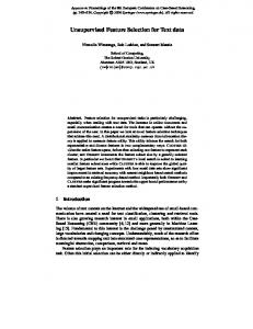
and express themselves conveniently and effortlessly. The pervasive use of social media produces massive data at an unprecedented speed. For example, 200 million tweets are posted per day1 ; 3,000 photos are uploaded per minute to Flickr2 ; and the number of Facebook users has increased from 100 million in 2008 to 800 million in 20113 . The massive and high-dimensional social media data poses new challenges to data mining tasks such as classification and clustering. One traditional and effective approach to handle high-dimensional data is feature selection [7, 18]. Feature selection aims to select relevant features from the highdimensional data for a compact and accurate data representation. It can alleviate the curse of dimensionality, speed up the learning process, and improve the generalization capability of a learning model [16, 19]. According to whether the training data is labeled or unlabeled, feature selection algorithms can be roughly divided into supervised and unsupervised feature selection. It is time-consuming and costly to obtain labeled data. Given the scale of social media data, we propose to study unsupervised feature selection. Unsupervised feature selection is particularly difficult due to the absence of class labels for feature relevance assessment [3]. Social media data adds further challenges to feature selection. Most existing feature selection algorithms work with “flat” attribute-value data which is typically assumed to be independent and identically distributed (i.i.d.). However, the i.i.d. assumption does not hold for social media data since it is inherently linked. Figure 1 shows a simple example of linked data in social media and its two data representations. Figure 1(a) shows 8 linked instances (u1 to u8 ). These instances usually form groups and instances within groups have more connections than instances between groups [31]. For example, u1 has more connections to {u2 , u3 , u4 } than {u5 , u6 , u7 , u8 }. Figure 1(b) is a conventional representation of attribute-value data: rows are instances and columns are features. For linked data, except for the conventional representation, there is link information between instances as shown in Figure 1(c). Linked data in social media presents both challenges and opportunities for unsupervised feature selection. In this work, we investigate: (1) how to exploit and model the relations among data instances, and (2) how to take advantage of these relations for feature selection using unlabeled data. One key difference between supervised and unsupervised fea1
http://techcrunch.com/2011/06/30/twitter-3200-milliontweets/ 2 http://www.flickr.com/ 3 http://en.wikipedia.org/wiki/Facebook
$
"
#
!
&
%
(a) Linked Users
' ' ! $ " # % &
….
….
'(
….
' ' ! $ " # % &
(b) Attribute-Value Data
….
….
….
'(
! $ " # % & ! $ " # % &
1 1
1 1
1
1
1
1
1
1 1
1 1
1 1
1 1
1 1
1
1
1 1
(c) Attribute-Value and Linked Data
Figure 1: A Simple Example of Linked Social Media Data ture selection is the availability of label information. If we change our perspective and consider label information as a sort of constraints in the learning space, we can turn both types of feature selection to a problem with the same intrinsic property: selecting features to be consistent with some constraints [35]. In supervised learning, label information plays the role of constraint. Without labels, other alternative constraints are proposed, such as data variance and separability, for unsupervised learning [27, 7, 4, 14, 35, 3]. However, most of them evaluate the importance of feature individually and neglect the feature correlation [36, 34]. In our attempt to address the challenges of unsupervised feature selection for linked social media data, we propose a novel framework of Linked Unsupervised Feature Selection (LUFS). Our main contributions are summarized below: • Employing social dimensions to exploit relations among linked data instances in groups and enable a concise mathematical model of these relations; • Introducing the concept of pseudo-class labels to develop alternative constraints for unsupervised feature selection using linked data; • Proposing a novel unsupervised feature selection framework, LUFS, for linked data in social media to exploit linked information in selecting features; • Evaluating LUFS extensively using datasets from realworld social media websites to understanding the working of LUFS. The rest of this paper is organized as follows. We formally define the problem of unsupervised feature selection for linked data in social media in Section 2; introduce our new framework of unsupervised feature selection, LUFS in Section 3, including social dimension regularization, optimization, and convergence analysis; present empirical evaluation with discussion in Section 4 and the related work in Section 5; and conclude this work in Section 6.
2. PROBLEM STATEMENT In this paper, scalars are denoted by lower-case letters (a, b, . . . ; α, β, . . .), vectors are written as lower-case bolded letters (a, b, . . .), and matrices correspond to boldfaced uppercase letters (A, B, . . .). Let u = {u1 , u2 , . . . , un } be the set of linked data (e.g., u1 to u8 in Figure 1) where n is the number of data instances and f = {f1 , f2 , . . . , fm } be the set of features where m is
the number of features. Let X = (x1 , x2 , . . . , xn ) ∈ Rm×n be the conventional representation of u w.r.t . f where xi (j) is the frequency of fj used by ui (e.g., Figure P1(b)). We assume that the data, X, is centered, that is, n i=1 xi = 0, which can be realized as X = XP where P = In − n1 1n 1⊤ n. For social media data, there also exist connections among its data instances. Let R ∈ Rn×n denote their connections where R(i, j) = 1 if ui and uj are linked, otherwise zero (e.g., the right subgraph in Figure 1(c)). In our work, we assume that the relationships among data instances form an undirected graph, i.e., R = R⊤ . With the above notations defined, the problem of unsupervised feature selection for linked data can be stated as: given n linked data instances, its conventional representation X, its link representation R, develop a method f , which can select a subset of relevant features f ′ from f by utilizing both X and R for these n linked instances, formally stated as, f : {f ; X, R} → {f ′ }.
(1)
The above is substantially different from the traditional task of unsupervised feature selection, formally defined as, f : {f ; X} → {f ′ }.
3.
(2)
UNSUPERVISED FEATURE SELECTION m−k
k
z }| { z }| { Set s = π(0, . . . , 0, 1, . . . , 1) where π(·) is the permutation function and k is the number of features to select where si = 1 indicates that the i-th feature is selected. The original data can be represented as diag(s)X with k selected features, where diag(s) is a diagonal matrix. The difficulty faced with unsupervised feature selection is due to lack of class labels. Hence, we introduce the concept of pseudo-class label to guide unsupervised learning. We assume that there is a mapping matrix W ∈ Rm×c , which assigns each data point with a pseudo-class label where c is the number of pseudo-class labels. The pseudo-class label indicator matrix is Y = W⊤ diag(s)X ∈ Rc×n . Each column of Y has only one nonzero entity, i.e., kY(:, i)k0 = 1 where k · k0 is the vector zero norm, counting the number of nonzero elements in the vector. Since X is centered, it is easy to verify that Y is also centered, n X i=1
yi =
n X i=1
n � �X W⊤ diag(s)xi = W⊤ diag(s) xi = 0. i=1
(3)
As shown above, both supervised and unsupervised learning tasks aim to solve the same problem: selecting features
consistent with given constraints. In the supervised setting, pseudo-class label information is tantamount to the provided label information; in the unsupervised setting, we seek pseudo-class label information from linked social media data. We discuss technical details of the proposed framework LUFS in the following subsection.
Social Dimension Extraction Constraints from Link Information
Mapping Matrix diag( )
%
"
# !
Laplacian Construction
=
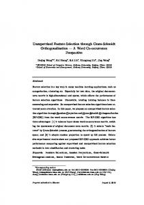
3.1 Social Dimensions for Linked Data First, we embark on dealing with linked data. In [30], social dimension is introduced as a means to integrate the interdependency among linked data and attribute-value data. Instances from different social dimensions are dissimilar while instances in the same social dimension are similar. Flattening linked data with social dimensions, traditional classification methods such as SVM obtain better performance for relational learning [30]. Social dimension extraction is a well-studied problem by social network analysis community [24, 11, 30]. In our work, we adopt a widely used algorithm, i.e., Modularity Maximization [24], which can formulated as: � max T r H⊤ MH (4) H⊤ H=I
where H ∈ RK×n is the social dimension indicator matrix, K is the number of social dimensions, and M is the modularity matrix defined as: dd⊤ (5) 2n where d is a degree vector, and di is the degree of ui . The standard K-means algorithm is performed to obtain the discrete-valued social dimension assignment, H(i, j) = 1, if uj is in the i-th dimension, and H(i, j) = 0, otherwise. Recall the simple example of linked data in Figure 1, we can extract two social dimensions, i.e, {u1 , u2 , u3 , u4 } and {u5 , u6 , u7 , u8 }. From Figure 1, we can observe that instances in the same social dimension have more connections. The discrete-valued social dimension indicator matrix, H, is: � � 1 1 1 1 0 0 0 0 H= 0 0 0 0 1 1 1 1 M=R−
Since social dimensions represent a type of user affiliations, inspired by Linear Discriminant Analysis, we define three matrices: within, between, and total social dimension scatter matrixes Sw , Sb , and St as follows: Sw = YY ⊤ − YFF⊤ Y ⊤ , Sb = YFF⊤ Y ⊤ , St = YY ⊤ ,
(6)
where F is the weighted social dimension indicator matrix, which can be obtained from H as below, 1
F = H(H⊤ H)− 2 ,
(7)
where the j-th column of F is given by hj
z }| { (0, . . . , 0, 1, . . . , 1, 0, . . . , 0) p Fj = . hj
(8)
where hj is the number of instances in the j-th social dimension. Instances in the same social dimension are similar and instances from different social dimensions are dissimilar. We
Feature Selection Matrix
Pseudo-Class Label Constraints from Attribute-Value Information
$
"
Figure 2: Illustration of the LUFS Framework can obtain a constraint from link information, social dimension regularization, to model the relations among linked instances, via the following maximization problem, � max T r (St )−1 Sb . (9) W
3.2
A Framework - LUFS
To take advantage of information from attribute-value part, i.e., X, similar data instances should have similar labels. According to spectral analysis [22], the constraint from attribute-value part can be formulated as the following minimization problem, min T r(YLY ⊤ )
(10)
where L = D − S is a laplacian matrix and D P is a diagonal matrix with its elements defined as D(i, i) = n j=1 S(i, j). S ∈ Rn×n denotes the similarity matrix based on X, obtained through a RBF kernel as, S(i, j) = e
−
kxi −xj k2 σ2
.
(11)
By introducing the concept of pseudo-class labels, constraints from both link information and unlabeled attributevalue data are ready for unsupervised feature selection. Our framework of linked unsupervised feature selection, LUFS, is conceptually shown in Figure 2 with our solutions to the two challenges (need to take into account of linked data and lack of labels): extracting constraints from both linked and attribute-value data, and then constructing pseudo-class labels through social dimension extraction and spectral analysis. Thus, our proposed framework, LUFS, is equivalent to solving the following optimization problem, � min T r(YLY ⊤ ) − αT r (St )−1 Sb , W,s
s.t.
s ∈ {0, 1}n , s⊤ 1n = k, kY(:, i)k0 = 1, 1 ≤ i ≤ n.
(12)
The problem in Eq. (12) is difficult to solve due to the two constraints. To make the problem solvable, we use some widely used relaxation methods. First, according to common relaxation for label indicator matrix [22], the constraint on Y is relaxed to orthogonality, i.e., YY ⊤ = Ic . With this relaxation, St in social dimension regularization is an identity matrix and T r(YY ⊤ ) = c is a constant. Social dimension regularization can be rewritten as, min T r(YY ⊤ ) − T r(YFF⊤ Y ⊤ ).
(13)
the reason for adding the constant in social dimension regularization will be explained later. With this relaxation, Eq. (12) can be relaxed to, min T r(YLY ⊤ ) + αT r(YY ⊤ − YFF⊤ Y ⊤ ) s.t.
s ∈ {0, 1}n , s⊤ 1n = k, YY ⊤ = Ic ,
(14)
The constraint on s makes Eq. (14) mixed integer programming [2], which is still difficult to solve. We observe that that diag(s) and W is as the form of diag(s)W in Eq. (14). Since s is a binary vector and m − k rows of the diag(s) are all zeros, diag(s)W is a matrix where the elements of many rows are all zeros. This motivates us to absorb the diag(s) into W, W = diag(s)W, and add ℓ2,1 norm on W to achieve feature selection as, min T r(W⊤ XLX⊤ W) + βkWk2,1 W � + αT r W⊤ X(In − FF⊤ )X⊤ W s.t.
W⊤ (XX⊤ + λI)W = Ic ,
(15)
where λI is added to make (XX⊤ +λI) nonsingular. kWk2,1 , controls the capacity of kWk and also ensures that kWk is sparse in rows, making it particularly suitable for feature selection. kWk2,1 is the ℓ2,1 -norm of kWk defined as [5], v m m uX X X u k t W2 (i, j) = kW(i, :)k2 . (16) kWk2,1 = i=1
j=1
i=1
Lemma 1. Assume E ∈ Rn×m is a matrix with orthonormal columns, that is, E⊤ E = Im , then In − EE⊤ is a symmetric and positive semidefinite matrix. Proof. It is easy to verify that In − EE⊤ is a symmetric matrix since (In − EE⊤ )⊤ = In − EE⊤ . Let E = UΣV⊤ be the Singular Value Decomposition (SVD) of E, where U ∈ Rn×n and V ∈ Rm×m are orthogonal. Σ = diag(σ1 , . . . , σm , 0, . . . , 0) is diagonal where σ1 ≥ σ2 ≥ . . . ≥ σm ≥ 0. Then we have, E⊤ E = Im ⇒ VΣ⊤ ΣV⊤ = VV⊤ ⇒ 1 ≥ σ1 ≥ σ2 ≥ . . . ≥ σm ≥ 0.
(17)
Then, In − EE⊤ = U(In − ΣΣ⊤ )U⊤ .
(18)
Since (In − ΣΣ⊤ ) is a diagonal matrix and the diagonal elements are all nonnegative, (In − ΣΣ⊤ ) is a positive semidefinite matrix. Thus U(In − ΣΣ⊤ )U⊤ is a semidefinite matrix, which completes the proof. The importance of Lemma 1 is two-fold. First, it explains why we need a constant on the social dimension regularization. Adding the constant can guarantee the convexity of the objective function in Eq. (15). Second, it paves the way for the following theorem for LUFS. Theorem 1. Eq. (15) can be converted into the following optimization problem, min W
f (W) = T r(W⊤ AW) + βkWk2,1 , s.t.
W⊤ BW = Ic ,
(19)
where A is a symmetric and positive semidefinite matrix and B is a symmetric and positive matrix. Proof. It suffices to show how to construct a symmetric and positive semidefinite matrix A and a symmetric and positive matrix B from Eq. (15). We construct B = XX⊤ +λI. It is easy to check that B is symmetric and positive when λ 6= 0 and then the constraint in Eq. (15) is converted into the one in Eq. (19). We construct A = XLX⊤ + αX(In − FF⊤ )X⊤ and then the objective function in Eq. (15) is converted into the one in Eq. (19). According to Lemma 1, (In − FF⊤ ) is symmetric and positive semidefinite; and according to the definition of Laplacian matrix, XLX⊤ is symmetric and positive semidefinite. Thus, A is symmetric and positive semidefinite, which completes the proof.
3.3
Optimization Algorithm for LUFS
In recent years, many methods have been proposed to solve the ℓ2,1 -norm minimization problem [21, 25, 34]. However, our problem is different from these existing ones due to the orthogonal constraint in Eq. (19). Hence, we propose the following algorithm, as shown in Algorithm 1, to optimize the problem in Eq. (19). Algorithm 1 LUFS Input: {X, R, α, β, λ, c, K, k} Output: k most relevant features 1: Obtain the social dimension indicator matrix H 1 2: Set F = H(H⊤ H)− 2 3: Construct S through Eq. (11) 4: Set L = D − S 5: Set A = XLX⊤ + αX(In − FF⊤ )X⊤ 6: Set B = XX⊤ + λI 7: Set t = 0 and initialize D0 as an identity matrix 8: while Not convergent do 9: Set Ct = B−1 (A + βDt ) 10: Set Wt = [q1 , . . . , qc ] where q1 , . . . , qc are the eigenvectors of Ct corresponding to the first c smallest eigenvalues 11: Update the diagonal matrix Dt+1 , where the i-th diagonal element is 2kWt1(i,:)k2 ; 12: Set t = t + 1 13: end while 14: Sort each feature according to kW(i, :)k2 in descending order and select the top-k ranked ones; In Algorithm 1, social dimension extraction and weighted social dimension indicator construction are from line 1 to line 2. The iterative algorithm to optimize Eq. (19) is presented from line 8 to line 13. The convergence analysis of the algorithm starts with the following two lemmas. Lemma 2. A ∈ Rm×m is symmetric and positive semidefinite and B ∈ Rm×m is symmetric and positive. If W ∈ Rm×c solves the following minimization problem: min
T r(W⊤ AW),
s.t.
W⊤ BW = Ic ,
W
then W consists of the eigenvectors of B to the c smallest eigenvalues.
(20) −1
A corresponding
Proof. The lemma can be easily obtained through Ky Fan Theorem [15].
Lemma 3.The following inequality holds if wti |ri=1 are non-zero vectors, where r is an arbitrary number. i X X kwt+1 k2 i kwt+1 k2 − i 2kw k t 2 i i ≤
X
kwti k2 −
i
X kwti k22 . 2kwti k2 i
(21)
Proof. The detailed proof can be found in our previous work [29]. With the above two lemmas, we develop the following theorem regarding the convergence of Algorithm 1. Theorem 2. At each iteration of Algorithm 1, the value of the objective function in Eq. (19) monotonically decreases. Proof. According to Lemma 2, Wt+1 in line 9 of Algorithm 1 is the solution to the following problem, � Wt+1 = min T r W⊤ (A + βDt )W , (22) W⊤ BW=I
which indicates that,
� � ⊤ T r Wt+1 (A + βDt )Wt+1 ≤ T r Wt⊤ (A + βDt )Wt .
Then we have the following inequality, X ⊤ T r(Wt+1 AWt+1 ) + β kWt+1 (i, :)k2 i
− β(
X
kWt+1 (i, :)k2 −
i
≤
T r(Wt⊤ AWt )
+β
X
Table 1: Statistics of the Datasets BlogCatalog Flickr Size 5,198 7,575 # of Features 8,189 12,047 # of Classes 6 9 # of Links 27,965 47,344 # Ave Degree 5.38 6.25
X kWt+1 (i, :)k22 ) 2kWt (i, :)k2 i
• UDFS [34] selects features in batch mode by simultaneously exploiting discriminative information and feature correlation. • Laplacian Score [14] evaluates the importance of a feature through its power of locality preservation. • SPEC [35] selects features using spectral regression. Following the existing evaluation practice for unsupervised feature selection, we assess LUFS in terms of clustering performance. We vary the numbers of selected features as {200, 300, 400, 500, 600, 700, 800, 900, 1000}. Each feature selection algorithm is first performed to select features, then K-means clustering is performed based on the selected features. Since K-means often converges to local minima, we repeat each experiment 20 times and report the average performance. The clustering quality is evaluated by two commonly used metrics, accuracy and normalized mutual information (NMI)6 . Denoting l(ci ) as the label of cluster ci , l(dj ) as the predicted label of the j-th document, the accuracy is defined as:
kWt (i, :)k2 Accuracy =
i
− β(
X
kWt (i, :)k2 −
i
X kWt (i, :)k22 (
i
2kWt i, :)k2
)
According to the lemma 3, we can obtain, f (Wt+1 ) ≤ f (Wt ),
(23)
K n 1 XX δ(l(ci ), l(dj )), n i=1 j=1
(24)
where δ(x, y) is the delta function that its value is 1 if x = y and 0 otherwise. Given two clusterings C and C ′ , the mutual information M I(C, C ′ ) is defined as:
which completes the proof.
M I(C, C ′ ) =
According to Theorem 2, Algorithm 1 converges to the optimal W for the problem in Eq. (19).
X
ci ∈C,c′j ∈C ′
p(ci , c′j ) log2
p(ci , c′j ) , p(ci )p(c′j )
(25)
and NMI is defined by
4. EXPERIMENTS AND DISCUSSION In this section, we present experiment details to verify the effectiveness of the proposed framework, LUFS. After introducing real-world social media datasets, we first evaluate the quality of selected features in terms of clustering performance, then study the effects of parameters on performance and finally further verify the constraint extracted from link information by social dimension.
4.1 Datasets, Baseline Methods, and Metrics We collect two datasets from real-world social media websites, i.e., BlogCatalog4 and Flickr5 , which are the subsets of two public available datasets used in [31] to uncover overlapping groups in social media. Some statistics of the datasets are shown in Table 1. LUFS is compared with the following three unsupervised feature selection algorithms, 4 5
http://www.blogcatalog.com http://www.flickr.com/
N M I(C, C ′ ) =
M I(C, C ′ ) , max(H(C), H(C ′ ))
(26)
where H(C) and H(C ′ ) represent the entropies of clusterings C and C ′ , respectively. Larger NMI values represent better clustering qualities.
4.2
Quality of Selected Features
In this subsection, we compare the quality of features selected by different algorithms using performance metrics given above. Conventionally, the parameters in feature selection algorithms are tuned via cross-validation. More discussion is given in Section 4.3. The resulting parameter values for LUFS are: {α = 0.1, β = 0.1, K = 70, c = 9} for Flickr while {α = 0.1, β = 0.1, K = 10, c = 6} for BlogCatalog. λ is used to make (XX⊤ + λI) nonsingular and according to empirical experience, we set λ to 0.01 in both 6 We use the source code from http://www.zjucadcg.cn/dengcai/Data/Clustering.html.
In addition to determining the number of selected features (which remains an open problem [34]), LUFS has four important parameters: the number of pseudo-class labels (c), the number of social dimensions (K), α (controlling social dimension regularization) and β (controlling ℓ2,1 -norm regularization). Hence, we study the effect of each of the four parameters (c, K, α, or β) by fixing the other 3 to see how the performance of LUFS varies with the number of selected features. The processes of parameter selection for Flickr and for BlogCatalog are similar and we present the details for Flickr to save space. Examples of experimental results are presented next. The number of pseudo-class labels c is varied from 2 to 20 with an incremental step of 1 while setting {α = 0.1, β = 0.1, K = 70}. The performance variation w.r.t. c and the number of features is depicted in Figure 3. Most of the time, the clustering performance first increases rapidly, reaches its best performance and decreases as c increases. This observation can be used to guide the determination of the optimal number of c for LUFS. Note that when c varies from 5 to 11, the clustering performance is not sensitive to c, especially when the number of selected feature is large. Fixing c = 9, α = 0.1 and β = 0.1, we vary the number of
0.25
0.2 30
NMI
Accuracy(%)
32
28
0.15
26 0.1 24
22 1000
0.05 1000 800 600 400
# of Features
10 11 8 9 6 7 4 5 2 3
12 13
14 15
20
800 600 400
# of Features
# of Pseudo−class
(a) Accuracy
10 11 8 9 6 7 4 5 2 3
12 13
14 15
20
# of Pseudo−class
(b) NMI
Figure 3: Number of Pseudo-class Labels vs Number of Features
0.2
0.15 30
NMI
Accuracy(%)
35
0.1
25 0.05
20 1000
0 1000 800
800
90 70
600
50 30
400
10
# of Features
90 70
600
50 30
400
10
# of Features
# of Social Dimension
(a) Accuracy
# of Social Dimension
(b) NMI
Figure 4: Number of Social Dimension vs Number of Features social dimensions from 10 to 100 with an incremental step of 10 and the performance variation w.r.t. the number of social dimensions and the number of features is demonstrated in Figure 4. Most of the time, with the increasing number of social dimensions, the performance first increases, reaches its peak value and degrades. This pattern can be used to determine the optimal number of social dimensions for LUFS. Fixing c = 9, K = 70 and β = 0.1, we vary α as {1e−6, 1e−3, 1e−2, 0.1, 0.3, 0.5, 0.7, 1}. The performance variation w.r.t. α and the number of features is depicted in Figure 5. The performance first increases and most of time, the peak values for both accuracy and NMI are achieved when α = 0.1, indicating the importance of social dimension regularization for LUFS. After α = 0.5, the performance is dramatically degraded, suggesting that only link information is not enough for LUFS. To study how β and the number of features affect the performance, we vary β as {1e−6, 1e−3, 1e−2, 0.1, 0.3, 0.5, 0.7, 1} and set c = 9, K = 70 and β = 0.1. The results are shown in Figure 6. We observe that the performance improves as β changes from 1e−3 to 1e−2 and from 1e−2 to 0.1. These results demonstrate the capability of the ℓ2,1 norm for feature selection.
35
0.2
0.15 30
NMI
4.3 Parameter Selection
34
Accuracy(%)
datasets. The comparison results of Flickr and BlogCatalog are shown in Tables 2 and 3, respectively. Note that the clustering performance with all features (i.e., without feature selection) is reported in the last columns. We observe the performance change with the numbers of selected features: it increases, reaches the peak, and then decreases. For example, LUFS achieves its peak values when the number of selected features are 500 and 300 for Flickr and BlogCatalog, respectively. The clustering performance with as few as 200 features is better than that with all features. For instances, LUFS obtains 10.51% and 18.68% relative improvement in terms of accuracy for Flickr and BlogCatalog, respectively. These results demonstrate that the number of features can be significantly reduced without performance deterioration. LapScore obtains comparable results with SPEC on both datasets. Most of time, UDFS outperforms both LapScore and SPEC, which is consistent with the results reported in [34]. LapScore and SPEC analyze features separately and select features one after another, which may omit the possible correlation between different features. While UDFS selects features in a batch mode and considers feature correlation. These observations support the conclusion in [3, 36, 34]: it is recommended to analyze data features jointly for feature selection. We observe that LUFS consistently outperforms these baseline methods on both datasets. For example, LUFS gains up to 19.82% and 11.44% relative improvement in terms of accuracy in Flickr and BlogCatalog, respectively. All baseline methods are based on the data i.i.d. assumption, which is not valid due to linked data in social media; and LUFS explicitly takes advantage of link information through social dimension regularization. We also note that with the increasing number of features, the improvement progressively decreases. Usually, LUFS achieves its best results sooner than baseline methods do. For example, LUFS achieves its best results in terms of accuracy in Flickr when 500 features are selected compared to 900 features for baseline methods.
0.1
25 0.05
20 1000
0 1000 800 600 400
# of Features
1e−6
1e−3
1e−2
0.1
0.3
0.5
0.7
1
800 600 400
α
(a) Accuracy
# of Features
1e−6
1e−3
1e−2
0.1
α
(b) NMI
Figure 5: α vs Number of Features
0.3
0.5
0.7
1
Table 2: Clustering Performance with Different Feature Selection Algorithms in Accuracy 200 300 400 500 600 700 800 900 1000 UDFS 26.29 26.41 27.02 27.29 27.55 27.95 28.41 31.07 30.79 LapScore 25.56 25.79 25.98 26.00 26.00 26.00 26.54 30.90 30.73 SPEC 26.29 26.29 26.29 26.29 26.29 26.29 26.29 26.35 25.62 LUFS 29.19 29.51 29.90 32.70 30.41 31.17 30.48 31.79 31.17 NMI 200 300 400 500 600 700 800 900 1000 UDFS 0.0361 0.0409 0.0702 0.0761 0.0811 0.0921 0.1062 0.1110 0.1200 LapScore 0.0302 0.0555 0.0691 0.0709 0.0662 0.0630 0.0694 0.0816 0.1056 SPEC 0.0361 0.0361 0.0361 0.0361 0.0361 0.0361 0.0361 0.0361 0.0559 LUFS 0.0951 0.1026 0.1489 0.1601 0.1582 0.1701 0.1614 0.1681 0.1596
Flickr 12047 25.49 25.49 25.49 25.49 12047 0.0296 0.0296 0.0296 0.0296
35
0.2
30
0.15
NMI
Accuracy(%)
Table 3: Clustering Performance with Different Feature Selection Algorithms in BlogCatalog Accuracy 200 300 400 500 600 700 800 900 1000 8189 UDFS 41.16 51.86 49.28 49.01 47.96 47.31 46.98 46.98 45.36 38.65 LapScore 41.07 49.83 48.93 48.59 47.75 46.84 46.69 46.76 45.09 38.65 SPEC 40.33 51.16 48.55 48.66 47.43 46.93 46.73 46.60 45.54 38.65 LUFS 45.87 55.70 52.72 51.41 50.93 50.68 50.35 48.95 47.20 38.65 NMI 200 300 400 500 600 700 800 900 1000 8189 UDFS 0.1842 0.1807 0.1789 0.1764 0.1741 0.1725 0.1744 0.1702 0.1673 0.1540 LapScore 0.1328 0.1755 0.1707 0.1746 0.1753 0.1757 0.1730 0.1675 0.1615 0.1540 SPEC 0.1819 0.1789 0.1768 0.1726 0.1765 0.1688 0.1742 0.1675 0.1654 0.1540 LUFS 0.2149 0.2121 0.2026 0.2040 0.2016 0.2014 0.1994 0.1927 0.1891 0.1540
25
20
0.1
0.05
15 1000
0 1000 800 600 400
# of Features
1e−6
1e−3
1e−2
0.1
0.3
0.5
0.7
1
800 600 400
β
(a) Accuracy
# of Features
1e−6
1e−3
1e−2
0.1
0.3
0.5
0.7
1
β
(b) NMI
Figure 6: β vs Number of Features Among the these four parameters of LUFS, β is most sensitive, the number of pseudo-class labels, the number of social dimensions and α are not so.
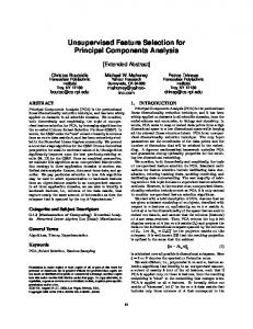
4.4 Probing Further A key contribution of LUFS to the performance improvement is to employ social dimensions extracted from linked data. Hence, we would like to probe further why the use of social dimensions works. One way is to investigate whether instances in the same social dimension are similar and instances from different social dimensions are dissimilar. Let z = {z1 , z2 , . . . , zK } be the K social dimensions given by the social dimension extraction algorithm, i.e., Modularity Maximization [24] here, with sizes of {n1 , n2 , . . . , nK } where Pni is number of instances in the i-th social dimension and i ni = n. To create reference groups in comparison with social dimensions, we also randomly divide these n instances into K groups with sizes of {n1 , n2 , . . . , nK }. Let ′ z′ = {z1′ , z2′ , . . . , zK } be the set of these randomly formed
groups with sizes of {n1 , n2 , . . . , nK } and then each group in z′ (e.g., zi′ ) corresponds to a social dimension in z (e.g., zi ). The label information is used earlier in assessing clustering performance. We use it again here. Let Y ′ be the class label indicator matrix. We center Y ′ as: Y ′ = Y ′ P. Two distance metrics are defined: Dwithin and Dbetween for within- and between-social dimension distance. Dwithin and Dbetween can be obtained from within social dimension scatter matrix Sw and between social dimension scatter matrix Sb , respectively, Dwithin = T r(Sw ), Dbetween = T r(Sb ).
(27)
For each specific number of social dimensions, K, we calculate Dwithin and Dbetween for z and z′ . Varying K from 2 to 100 with an incremental step of 1, we obtain 99 pairs of Dwithin and 99 pairs of Dbetween . The results for Flickr and BlogCatalog are shown in Figure 7. Dwithin and Dbetween change much faster for social dimensions, comparing with groups of random assignment. Moreover, Dwithin of a social dimension is much smaller than that of a random assignment group, thus, instances in the same social dimension are of similar labels. Dbetween of a social dimension is much larger than that of a random assignment group, indicating that instances from different social dimensions are dissimilar. We also perform a two-sample t-test on these pairs of Dwithin of z and z′ at significant level 0.001. The null hypothesis, H0 , is that there is no different between these pairs; the alternative hypothesis, H1 , is that Dwithin of a social dimension is less than that of the corresponding random assignment group. The t-test results, p-values, are 6.0397e−060 and 8.2406e−083 on Flicker and BlogCatalog,
1400
600 Social Dimension Random Assignment
Social Dimension Random Assignment 500
Between Distance
Within Distance
1300
1200
1100
1000
900
800
400
300
200
100
0
20
40
60
80
0
100
0
20
# of Social Dimensions
40
60
(a) Dwithin for Flickr
250 Social Dimension Random Assignment
Social Dimension Random Assignment 200
Between Distance
500
Within Distance
100
(b) Dbetween for Flickr
550
450
400
350
300
80
# of Social Dimensions
150
100
50
0
20
40
60
80
100
# of Social Dimensions
0
0
20
40
60
80
100
# of Social Dimensions
(c) Dwithin for BlogCatalog (d) Dbetween for BlogCatalog
Figure 7: Within and Between Distance Achieved by Social Dimension and Random Assignment respectively. Hence, there is strong evidence to reject the null hypothesis. We conduct a similar test for the pairs of Dbetween , and there is strong evidence to support that Dbetween of a social dimension is significantly larger than that of its counterpart, a random assignment group. The evidence from both figures and t-test confirms the positive impact of the constraint from link information via social dimensions.
5. RELATED WORK Traditionally, feature selection algorithms can be either supervised or unsupervised [7, 20] based on the training data being labeled or unlabeled. Supervised feature selection methods [20] can be broadly categorized into the wrapper models [8, 17] and the filter models [13, 26]. The wrapper model uses the predictive accuracy of a predetermined learning algorithm to determine the quality of selected features. These methods can be egregiously expensive to run for data with a large number of features [6, 12]. The filter model separates feature selection from classifier learning so that the bias of a learning algorithm does not interact with the bias of a feature selection algorithm. It relies on measures of the general characteristics of the training data such as distance, consistency, dependency, information, and correlation [13]. Many researchers paid great attention to developing unsupervised feature selection [32, 14, 4]. Unsupervised feature selection [14, 7, 35] is a less constrained search problem without class labels, depending on clustering quality measures [10, 9], and can eventuate many equally valid feature subsets. With highdimensional data, it is likely to find many sets of features that seem equally good without considering additional constraints. Another key difficulty is how to objectively measure the results of feature selection. A wrapper model is proposed in [7] to use a clustering algorithm in evaluating the quality of feature selection. Recently, sparsity regularization, such as the ℓ2,1 -norm of
a matrix [5], in dimensionality reduction has been widely investigated and applied to feature selection including multitask feature selection [1, 21], robust joint ℓ2,1 -Norms [25], spectral feature selection [35], discriminative unsupervised feature selection [34]. Through sparsity regularization, feature selection can be embedded in the learning process. The first attempt to select features on social media data is LinkedFS [29], a supervised algorithm. Various relations (coPost, coFollowing, coFollowed and Following) are extracted following social correlation theories [23]. LinkedFS significantly improves the performance of feature selection by incorporating these relations into feature selection. However, LinkedFS and LUFS are distinctively different. First, LinkedFS is formally stated as: f : {f ; X, Y} → {f ′ } where Y contains the label information, while LUFS is a unsupervised feature selection algorithm. Second, LinkedFS exploits relations individually while LUFS employs relations as groups via social dimensions.
6.
CONCLUSION
Linked data in social media presents new challenges to traditional feature selection algorithms, which assume the data instances to be independent and identically distributed. In this paper, we propose a novel unsupervised feature selection framework, LUFS, for linked data in social media. We utilize a recent developed concept of social dimensions from social network analysis to extract relations among linked data as groups, and define social dimension regularization inspired by Linear Discriminant Analysis to mathematically model these relations. We then propose the concept of pseudoclass labels to develop a new unsupervised feature selection framework by ensuring that instances in a social dimension are similar, and otherwise dissimilar. Experimental results on two datasets from real-world social media websites show that the proposed method can effectively exploit link information in comparison with the state-of-the-art unsupervised feature selection methods. In social media networks, the availability of various link formation can lead to networks with relationships of different strengths [33, 28], which means that weak links and strong links are often mixed together. We plan to incorporate tie strength prediction into LUFS to further exploit link information. Also we believe that the concept of pseudo-class label introduced in the paper is a powerful means to effectively constrain the learning space of unsupervised feature selection and can be extended to different applications without labeled data but additional information.
Acknowledgments The work is, in part, supported by ARO (#025071) and NSF (#0812551).
7.
REFERENCES
[1] A. Argyriou, T. Evgeniou, and M. Pontil. Multi-task feature learning. NIPS, 19:41, 2007. [2] S. Boyd and L. Vandenberghe. Convex optimization. Cambridge Univ Pr, 2004. [3] D. Cai, C. Zhang, and X. He. Unsupervised feature selection for multi-cluster data. In KDD, pages 333–342. ACM, 2010.
[4] C. Constantinopoulos, M. Titsias, and A. Likas. Bayesian feature and model selection for gaussian mixture models. TPAMI, pages 1013–1018, 2006. [5] C. Ding, D. Zhou, X. He, and H. Zha. R 1-pca: rotational invariant l 1-norm principal component analysis for robust subspace factorization. In Proceedings of the 23rd international conference on Machine learning, pages 281–288. ACM, 2006. [6] R. Duda, P. Hart, D. Stork, et al. Pattern classification, volume 2. wiley New York, 2001. [7] J. Dy and C. Brodley. Feature selection for unsupervised learning. Journal of Machine Learning Research, 5:845–889, 2004. [8] J. G. Dy and C. E. Brodley. Feature subset selection and order identification for unsupervised learning. In Proceedings of the Seventeenth International Conference on Machine Learning, pages 247–254, 2000. [9] J. G. Dy and C. E. Brodley. Visualization and interactive feature selection for unsupervised data. In KDD, pages 360–364, 2000. [10] J. G. Dy, C. E. Brodley, A. C. Kak, L. S. Broderick, and A. M. Aisen. Unsupervised feature selection applied to content-based retrieval of lung images. IEEE Transactions on Pattern Analysis and Machine Intelligence, 25(3):373–378, 2003. [11] E. Erosheva, S. Fienberg, and J. Lafferty. Mixed-membership models of scientific publications. Proceedings of the National Academy of Sciences of the United States of America, 101(Suppl 1):5220, 2004. [12] I. Guyon, J. Weston, S. Barnhill, and V. Vapnik. Gene selection for cancer classification using support vector machines. Machine learning, 46(1):389–422, 2002. [13] M. Hall. Correlation-based feature selection for discrete and numeric class machine learning. In Proceedings of Seventeenth International Conference on Machine Learning (ICML-00). Morgan Kaufmann Publishers, 2000. [14] X. He, D. Cai, and P. Niyogi. Laplacian score for feature selection. NIPS, 18:507, 2006. [15] R. Horn and C. Johnson. Matrix analysis. Cambridge Univ Pr, 1990. [16] G. John, R. Kohavi, and K. Pfleger. Irrelevant feature and the subset selection problem. In W. Cohen and H. H., editors, Machine Learning: Proceedings of the Eleventh International Conference, pages 121–129, New Brunswick, N.J., 1994. Rutgers University. [17] Y. Kim, W. Street, and F. Menczer. Feature selection for unsupervised learning via evolutionary search. In KDD, pages 365–369, 2000. [18] H. Liu and H. Motoda. Computational methods of feature selection. Chapman & Hall, 2008. [19] H. Liu and L. Yu. Toward integrating feature selection algorithms for classification and clustering. IEEE Transactions on Knowledge and Data Engineering, 17(4):491, 2005. [20] H. Liu and L. Yu. Toward integrating feature selection algorithms for classification and clustering. IEEE Trans. on Knowledge and Data Engineering, 17(3):1–12, 2005. [21] J. Liu, S. Ji, and J. Ye. Multi-task feature learning via
[22] [23]
[24]
[25]
[26]
[27] [28]
[29]
[30]
[31]
[32]
[33]
[34]
[35]
[36]
efficient l 2, 1-norm minimization. In Proceedings of the Twenty-Fifth Conference on Uncertainty in Artificial Intelligence, pages 339–348. AUAI Press, 2009. U. Luxburg. A tutorial on spectral clustering. Statistics and Computing, 17(4):395–416, 2007. P. Marsden and N. Friedkin. Network studies of social influence. Sociological Methods and Research, 22(1):127–151, 1993. M. E. J. Newman and M. Girvan. Finding and evaluating community structure in networks. Physical review E, 69(2):26113, 2004. F. Nie, H. Huang, X. Cai, and C. Ding. Efficient and robust feature selection via joint l21-norms minimization. NIPS, 2010. H. Peng, F. Long, and C. Ding. Feature selection based on mutual information: criteria of max-dependency, max-relevance, and min-redundancy. IEEE Transactions on pattern analysis and machine intelligence, pages 1226–1238, 2005. V. Roth and T. Lange. Feature selection in clustering problems. NIPS, 16:473–480, 2004. J. Tang, H. Gao, and H. Liu. mtrust: Discerning multi-faceted trust in a connected world. In The ACM international conference on Web search and data mining, 2012. J. Tang and H. Liu. Feature selection with linked data in social media. In SIAM International Conference on Data Mining, 2012. L. Tang and H. Liu. Relational learning via latent social dimensions. In KDD, pages 817–826. ACM, 2009. X. Wang, L. Tang, H. Gao, and H. Liu. Discovering overlapping groups in social media. In 2010 IEEE International Conference on Data Mining, pages 569–578. IEEE, 2010. L. Wolf and A. Shashua. Feature selection for unsupervised and supervised inference: the emergence of sparsity in a weighted-based approach. Journal of Machine Learning Research, 6:1855–1887, 2005. R. Xiang, J. Neville, and M. Rogati. Modeling relationship strength in online social networks. In Proceedings of the 19th international conference on World wide web, pages 981–990. ACM, 2010. Y. Yang, H. Shen, Z. Ma, Z. Huang, and X. Zhou. L21-norm regularized discriminative feature selection for unsupervised learning. In Proceedings of the Twenty-Second International Joint Conference on Artificial Intelligence, 2011. Z. Zhao and H. Liu. Spectral feature selection for supervised and unsupervised learning. In Proceedings of the 24th international conference on Machine learning, pages 1151–1157. ACM, 2007. Z. Zhao, L. Wang, and H. Liu. Efficient spectral feature selection with minimum redundancy. In Proceedings of the Twenty-4th AAAI Conference on Artificial Intelligence (AAAI), 2010.