Journal of Physical Science, Vol. 19(1), 13–29, 2008
13
Mixing Behavior of Binary Polymer Particles in Bubbling Fluidized Bed S.M. Tasirin, S.K. Kamarudin* and A.M.A. Hweage Department of Chemical and Process Engineering, Universiti Kebangsaan Malaysia, 43600 UKM Bangi, Selangor, Malaysia *Corresponding author:
[email protected] Abstract: Fluidized bed mixer offers the most efficient and economical process compared to other mixers. However, less effort has been devoted to understand the local behavior of the solids in fluidized bed, partly due to the lack of reliable experimental methods. Thus, the objective of this paper was to view the local mixing behavior and property of a free flow polymer binary mixture in bubbling fluidized bed. In this work, an experimental study of mixing process of free flowing polymers binary mixtures at different densities and colors in bubbling fluidized were investigated. The mixing properties were studied by analyzing the variation of the proportions of the marked particles with time and position in the bed. The variation of mixture composition based on the samples incorporated into Lacey mixing index that describes the degree of mixing of the particle at particular time. This method enables the assessment of the overall mixing behavior in terms of the rate of mixing (through estimation of the time required for the mixing index to increase from zero to a certain value) and with the degree of mixing at the mixing equilibrium stage. Finally, the parameters were optimized. Results showed that gas velocity and bed depth were important parameters influencing the solids mixing in the bubbling fluidized bed. From the results, complete mixing of binary polymer particles was attained at a bed depth of 17 cm and gas velocity of 1.38 Umf in the fluidized bed. Keywords: polymer particles, mixing, fluidized bed
1.
INTRODUCTION
Fluidized bed mixer offers the natural mobility afforded particles in the fluidized bed. The mixing is largely convective with the circulation patterns set up by the bubble motion within the bed.1 An important feature of the fluidized bed mixer is the ability of conducting several procedures like mixing, reaction, coating, drying etc., is single vessel. On the other hand, based on the energy consumption analysis, it has been found that a fluidized bed mixer offers the most efficient and economical process compared to other mixers. However, less effort has been devoted to understand the local behavior of the solids in the fluidized bed, partly due to lack of reliable experimental methods.2–5 Quantification of solids flow pattern and solids mixing is very essential for proper design and scale-up of fluidized beds.6 The basic mechanism of solid
Mixing Behavior of Polymer Particles
14
mixing in bubbling fluidized bed is well-understood but it is still not possible to predict the effect of operating parameters on the degree of mixing in a fluidized bed.7 Thus, the objectives of this study were:
To study the mixing behavior and property of the free flow polymer binary mixtures.
To determine the optimum operating conditions in the final mixture of specified compositions of polymer A and B as 3:1, respectively.
To investigate the mixing performance of free flow polymer binary mixture in bubbling fluidized bed.
2.
THEORITICAL BACKGROUND
The end use of particle mixture will determine the quality of mixture required. For any manufacturing process that involves mixing of solid particles, the level of in-homogeneity is important for determination of the quality for the final product. It is even more difficult to obtain a homogeneous mixture when particles are at different size or density.6 The end use imposes a scale of scrutiny on the mixture defined as the maximum size of the regions for segregation in the mixture that would cause it to be regarded as imperfectly mixed.8 Sampling and quality of analysis of the mixture require the application of statistical methods. The segregation index calculation is frequently used to describe quantitatively the powder mixtures. Most of these indices have been developed based on statistical analysis and especially on the definitions of specified property. These mixing indices usually describe the closeness of a mixture to a "completely random mixture". Most of the definitions are based on the standard deviation expressing the difference in composition throughout the mixture.9–11 Nevertheless, the standard deviation or variance depends largely on the sample size, which should be identical to the scale of scrutiny at which end used properties are to be evaluated.11,12 The following mixing index is directly proportional to the standard deviation. N is the number of samples, containing n particles, estimate the mixture composition value as given in Equation (1):9
Journal of Physical Science, Vol. 19(1), 13–29, 2008 −
y= While
1 N ∑ yi N i =1
15
(1)
− y th
is an estimation of the mixture content in a definite (key) component, yi is the i value of this proportion in a sample. We can use the standard deviation for the composition of the samples taken from the mixture as a measure of the quality of the mixture. Thus a low standard deviation indicates a narrow spread in composition of samples and therefore predicts a good mixing. The sample variance, S2 is given by Equation (2):
S2 =
− N 1 ∑( yi − y) ( N − 1) i =1
(2)
The value of standard deviation, S determined from Equation (2) only the estimation value for the actual standard deviation of the mixture, σ . Different sets of samples will give different estimated value. The actual value of the standard deviation for a random binary mixture, variance (σR ) is given as Equation (3).9,10,13
⎡ P (1 − P ) ⎤ n ⎥⎦
σ R2 = ⎢ ⎣
(3)
where P and (1-P) are the fraction of the two components in the mixture and n is the number of particles in each sample. Equation (3) is applicable for a random mixture in which each component has a distribution of particle size. However the number of particles in a given mass of sample depends on the size distribution of the components. Thus, for a binary mixture of spherical particles of components A and B with proportions of PA and PB, respectively, the number of particles of A or B per unit mass of component A or B, respectively is given by Equation (4). B
⎡ M ass of particles in ⎤ ⎢ each size range ⎥ ⎣ ⎦
=
⎡ N um ber of particles ⎤ ⎡ M ass of one ⎤ ⎢ in size range ⎥⎢ ⎥ ⎣ ⎦ ⎣ particle ⎦
(4)
M = ρ pV
(5)
and
Mixing Behavior of Polymer Particles
where V =
16
πd 3p
= volume of one particle, n = number of particles in size range, 6 ρp = particle density, M = mass of one particle, and dp = the arithmetic mean of adjacent sieve size. The actual standard deviation for a completely segregated system (in this case a completely unmixed system, upper limit) is given by variance, σ0 as in Equation (6).9,10,13.
σ02 = P (1 − P )
(6)
The actual values of mixture variance lie between these two extreme values namely σ02 and σR2 . Due to that, in this study, Lacey mixing index was used to predict the degree of mixing.9 The variance for experimental data, S 2 are comparable to σ02 and σ02 for binary mixtures of identical particles.
M=
σ02 − σ2 σ02 − σR2
(7)
with σ = the variance of the mixture between fully random and completely segregated mixtures, σ02 = is the upper limit (completely segregated) of mixture 2
variance, σR2 = is the lower limit (randomly mixed) of mixture variance, M = the Lacey mixing index. A Lacey mixing index of zero predicts a complete segregation of the particles while a value of unity would represent a completely random mixture. Particle values for this mixing index are found in the range of 0.75 to 1.0.1
3.
METHODOLOGY
3.1
Physical Properties of Feed Particles
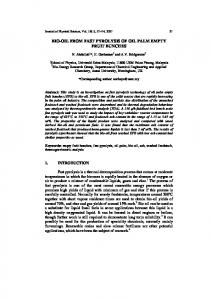
Two types of polymer particles referred as polymer A (white) and B (black) were used as the feed sample in this study. Table 1 and Figure 1 present the physical properties of the two different polymers.
Journal of Physical Science, Vol. 19(1), 13–29, 2008
17
Table 1: Physical properties of polymers used in this study. Parameter
Polymer A (white)
Polymer B (black)
−
Mean particle size, d p (µm)
3465
3502
Particle density, ρp (kg/m3)
923
1105
Bulk density, ρba (kg/m3)
617
745
D
D
4750–2360
4750–2360
Geldart classification on size distribution −
Size range, d p (µm)
(a)
(b)
Figure 1: Samples of the solids used in this study (a) polymer particles A (white) and (b) polymer particles B (black).
3.1.1
Size distribution analysis
In this study, the size distribution analysis was carried out using sieve (Testmate, Malaysia) with apertures of 4750, 4000, 3350, 2800 and 2360 µm. −
The arithmetic mean of the adjacent sieves, d pi and the mean particle size, d p of the bulk particles are calculated as following:
d pi =
di + di +1 2 −
dp =
, i = 1, 2, 3,....., n
1 ∑(mi / d pi )
(8) (9)
Mixing Behavior of Polymer Particles
18
where mi is the weight fraction for the mean particle size, dpi. 3.1.2
Particle density, ρp measurement using a pycnometer
The density of non-porous solid particles in this study was measured by a gas pycnometer (Quantachorme, USA). Table 2 shows the particle density, ρp for both polymers A (white) and B (black). It is observed that the particle density reduces as the particle size decrease. The average values of ρp used in this study are as per listed in Table 1. 3.2
Mixing Properties of Particles in Fluidized Bed
3.2.1
Apparatus
Figure 2 shows the experimental set-up of the mixing fluidized bed. The system consisted of a Perspex cylinder, 143 mm in diameter and 1000 mm length. A pressure probe connected to a water manometer that measured the pressure drop across the bed. A transparent scale was attached to the bed wall to provide direct bed expansion measurement. The gas inlet system comprises with multi speed motor, a flow meter and a gas distributor system as suggested by Geldart.14 The total number of orifice was calculated as 217. Compressed air at 0.4 to 0.6 MPa was supplied from a central blower to fluidize the air. Table 2: The densities for each size fraction of polymer. No.
Range size (µm)
dp (µm)
dv (µm)
White particle ρ (kg/m3)
Black particle ρ (kg/m3)
1
4750–4000
4375
4944
1127.7
968.4
2
4000–3350
3675
4153
951.4
1115.6
3
3350–2800
3075
3475
895.0
1002.1
4
2800–2360
2580
2915
708.1
885.1
Journal of Physical Science, Vol. 19(1), 13–29, 2008
19
D = 0.143 m D = 0.143 m
L=1m
0.18 m
FIGURE 3.7 Photograph the fluidised bed used Figure 2: Experimental set-up for of bubbling fluidized bed in in this this work. study.
3.2.2
Experimental method
Batch experiments were carried out in Perspex fluidized bed column (Fig. 2). Table 3 listed the series of experimental work carried out in this study. The critical bed depth, Hmsc for slugging bed was obtained at 18.98 cm using Equation (10).1 Due to the bed depths lower than Hmsc were chosen in this work namely, 10, 15 and 17 cm, in order to make sure no slugging phenomena occur in the bed. 1.90 ⎡ H msc ⎤ − ⎢ D ⎥≤ ⎣ ⎦ (ρ d p )0.3 p
(10)
Mixing Behavior of Polymer Particles
20
Table 3: Experimental series for mixing in a fluidized bed. Parameter
Series of experimental work
Umf (m/s)
1.35
Operating gas velocity
Umf, 1.15 Umf , 1.38 Umf
Bed depth, H (cm)
10, 15, 17
Bed weight, m (kg)
1.042, 1.563, 1.772
Hmsc (cm)
18.98
Duration, t (s)
5, 10, 12, 15, 20, 30
3.2.3
Sampling
Side-sampling thief method was employed to assess the performance of solids-gas fluidized bed mixer. It removes sample portions from different locations of the mixture in the fluidized bed. In this case, the sample thief has three samples apertures that can be opened and closed in a controlled manner. Once the thief probe is fully inserted into the powder mixture, the apertures are opened allowing powder to flow into them. The apertures are then closed and the probe is withdrawn. On the basis of their color, the components were separated by hand and the particles were counted.14
4.
RESULTS AND DISCUSSION
The following section shows the effect of some parameters like superficial velocity, pressure drop, mixing time and others toward the mixing process in fluidized bed. In addition, it also presents the best bed depth to produce a homogeneous mixture at optimum mixing time. Figure 3 presents the results obtained for pressure drop across the bed as the superficial gas velocity was increased. At relatively low superficial gas velocity, the pressure drop across the bed was approximately proportional to the superficial gas velocity. However, the pressure drop values were constant at above the minimum fluidization velocity, Umf. The consistency in pressure drop showed that the fluidizing gas stream had fully supported the weight of the whole bed in the dense phase. Thus Umf reached when the drag force of the up-wards fluidizing air equals to the bed weight. In this case, Umf was determined as 1.35 ms–1.
Journal of Physical Science, Vol. 19(1), 13–29, 2008
21
900 800
Pressure drop, P, [Pa
Pressure Drop, P (Pa)
700 600
(Umf)experimental = 1.35 m/s
500 400 300 200 100 0 0
0.5
1
1.5
2
Superficial gas velocity, U, [m/s]
Superficial Gas Velocity, U (m/s)
Figure 3: Pressure drop versus superficial gas velocity (at increasing gas flow rate) for initially mixed/segregated mixtures.
Figure 4 shows the results of mixing index at different mixing time for different operating gas velocities. It observed that for all the cases, the mixing index gradually increased until it reaches the equilibrium stage for mixing process. For superficial gas velocity at 1.15 Umf and 1.38 Umf the M gives the value as 0.99 while the at the superficial gas velocity equals to Umf, the M values are between 0.6–0.7. This proved that a good mixing process can be obtained at higher gas superficial velocity than Umf. Besides, it is observed that the superficial velocity greater that Umf needs a shorter time to reach the mixing equilibrium stage. It agrees with the general trend reported in the literatures. 15,16, 17 The observations from the Figure 4 showed that the optimum mixing time depends on the superficial gas velocity. 1.2
MIXING INDEX, M (-)
Mixing Index, M (-)
1
0.8
0.6
0.4
0.2 Umf
1.15Umf
1.38Umf
0 0
5
10
15
20
25
30
35
MIXING TIME, t (sec)
Mixing Time, t (s)
Figure 4: Effect of mixing time on Lacey mixing index at different gas velocity and bed depth = 17 cm.
Mixing Behavior of Polymer Particles
22
Figure 5 shows an illustrative example of the mixing process for polymer particles in the bed depth of 17 cm. The superficial gas velocity was taken as 1.38 Umf. The bed was first operated for about 5 s in order to ensure the steady state operation. The time was set to zero, t = 0 s at the point where the black and white colored particles are completely segregated. As the mixing process proceeds, it is observed that particle A and B are partially mixed. It was observed the mixing process was improving after the about 9 s from the initial condition.
t=0s
t=1s
t=6s
t=3s
t=9s
t=5s
t = 12 s
Figure 5: An illustration of the process of mixing (bed depth = 17 cm, superficial gas velocity = 1.38 Umf).
Journal of Physical Science, Vol. 19(1), 13–29, 2008
23
Figure 6 illustrates the mixing process in bubbling fluidized bed where the bubble motion drives the solids motion. The bubbles carried the particles upward in their wakes and drift. Particles move upward at the central part of the bed. However, it is observed that the particle is moving downward near the wall side of the bed. This vertical movement of the particle is called as convective mixing. Lateral mixing occurs mainly at the top of the bed where the bubble burst (Fig. 6b). Figures 7 depict the variation of mixing index as a function of time and depth height. It showed that the mixing index increases when the bed depth decreases at low velocity. However, it is noticeable that the mixing index increases, as the gas velocity increases (Fig. 4). This shows that a good mixing process is very dependent to the bed depth and the gas velocity. From Figure 8, it is observed that at a sufficiently high gas velocity (namely 1.38 Umf in this case) capable to minimize the effect of the bed depth for solid mixing process. Bust bubble Bubbles
Bubble
Bubble
(a)
(b)
Figure 6: An illustration the bubbles behavior of polymers mixing. 1
Mixing Index, M (-)
0.9 0.8 0.7 0.6 0.5 0.4 0.3 0.2 10 cm
0.1
15 cm
17 cm
0 0
5
10
15
20
25
30
35
Mixing Time, t (s)
(a) Figure 7: Effect of bed depth on Lacey index in fluidized bed with gas velocity equals (a) Umf, (b) 1.15 Umf and (c) 1.38 Umf.
Mixing Behavior of Polymer Particles
24
1.2
MIXING INDEX, M (-)
Mixing Index, M (-)
1 0.8 0.6 0.4 0.2
10 cm
15 cm
17 cm
0 0
5
10
15
20
25
30
35
MIXING TIME, t (sec)
Mixing Time, t (s)
(b)
1.2
M IX IN G IN DE X , M
Mixing Index, M (-)
1
0.8
0.6
0.4
0.2 10 cm
15 cm
17 cm
0 0
5
10
15
20
25
30
35
M IX IN G TIM E , t (sec)
Mixing Time, t (s)
(c) Figure 7: (continued)
Figure 8 shows the images taken at different bed depths for each mixture. Resulting images revealed a completely homogeneous comparison for mixing at 1.38 Umf for 17 cm bed depth. Nevertheless, this mixture was spouted, as in Figure 9. Spouting is a condition which may occur when a single hole is used to admit the gas rather than a porous plate or multi-hole distributor,17 or for group D (spoutable powder) and the larger group B particles (sand-like).18
Journal of Physical Science, Vol. 19(1), 13–29, 2008
(a)
H = 15 cm
25
(b)
t=5s
H = 17 cm
(c)
t=5s
H = 17 cm
t=9s
Figure 8: Influence of bed depth on the degree of homogeneity of mixtures with time. Spout
t = 12 s Figure 9: Photograph showing the spout of homogeneous mixture at bed depth of 17 cm and gas velocity of 1.38 Umf.
4.1
Process Optimization
In fluidized bed, the optimal mixing process reflected from low energy consumption. For solid mixing, the lowest energy consumption is predicted at the lowest value of the dimensionless factor, K. Thus, Figure 10 proved that the bed depth at 17 cm with gas velocity of 1.38 Umf is the optimum operation, since it gives the lowest value of K and at high value of Lacey mixing index, 0.99.
Mixing Behavior of Polymer Particles
26
0.45
Dimensionless Factor, K (-)
0.4 0.35 0.3 0.25 0.2 0.15 0.1
10cm,Umf 15cm,Umf 17cm,Umf
0.05
10cm,1.38Umf 15cm,1.38Umf 17cm,1.38Umf
10cm,1.15Umf 15cm,1.15Umf 17cm,1.15Umf
0 0
0.2
0.4
0.6
0.8
1
1.2
Lacey Mixing Index, M (-)
Figure 10: Dimensionless mixing factor, K vs. Lacey mixing index, M (-) for fluidized bed.
5.
CONCLUSION
Solids mixing is an important process in many industrial like pharmaceutical, chemical, petrochemical, foodstuffs, plastics, metallurgical, fertilizers, grain etc. but less effort has been devoted to understand the local behavior of the solids in mixing process and method to represent the mixing quality. However, this study proved that, Lacey index, M capable to determine the performance of particle mixing and recommend the bubbling fluidized as a good alternative for solid mixing. Finally the optimum parameters for solid mixing in this study was determined the bed depth of 17 cm with the gas velocity 1.38 Umf that give highest Lacey mixing index. This study also proved that the superficial velocity of air higher that Umf, capable to reduce the effect of bed height to the mixing process.
Appendix A dp −
dp dv E, E1 g Hmsc H K M mi N n, np P ∆P Q S S2 t V U Umf yi −
y Greek Letters ρba ρg ρp
cross-sectional area of column the arithmetic mean of adjacent sieve size (particle size) mean sieve particle size
m2 µm µm
diameter of sphere having same volume as a particle specific energy consumption acceleration due to gravity (9.81 N/sec2) critical bed height Height of gently settled bed Dimensionless mixing factor Lacey mixing index weight fraction of the particle of size range dpi number of sample number of particles in each sample fraction of the key component in a binary mixture pressure drop across the bed gas flow rare estimate of standard deviation of sample estimate of variance time volume of one particle superficial gas velocity velocity at minimum fluidization ith value of the proportion of one component in the samples (composition of samples by weight fraction) the mixture composition (mean value of sample composition by weight)
m J/kg N/sec2 cm, m cm, m Pa m3/s s, min m3 m/s m/s
kg/m3 kg/m3 kg/m3 -
σR
2
bulk density of particles gas density particle density lower limit (randomly mixed) of mixture variance
σ0
2
upper limit (completely segregated) of mixture variance
-
-
Mixing Behavior of Polymer Particles
28
6.
REFERENCES
1.
Rhodes, M.J. (1998). Introduction to particle technology. Chichester: John Wiley. Ohki, K. & Shirai, T. (1975). Particle velocity in fluidised bed. In D. Keairns (Ed.). Fluidisation technology. Vol. 1. Washington: Hemisphere. Cody, G.D., Goldfarb, D.J., Storch, G.V. & Norris, A.N. (1996). Particle granular temperature in gas fluidised beds. Powder Technology, 87, 211–232. Menon, N. & Durian, D.J. (1997). Particle motions in a gas-fluidised bed of sand. Physical Review Letters, 79, 3407–3410. Godfory, L., Larachi, F. & Chaouki, J. (1999). Position and velocity of a large particle in a gas/solid riser using the radioactive particle tracking technique. Canadian Journal of Chemical Engineering, 77, 253–261. Stein, M., Ding, Y.L., Seville, J.P.K. & Parker, D.J. (2000). Solids motion in bubbling gas fluidised beds. Chemical Engineering Science, 55, 5291–5300. Garncarek, Z., Przybylski, L., Botterill, J.S.M., Bridgwter, J. & Broadbent, C.J. (1994). A measure of the degree of in homogeneity in a distribution and its application in characterizing the particle circulation in a fluidised bed. Powder Technology, 80(3), 221. Danckwerts, P.V. (1952). The definition and measurement of some characteristics of mixtures. Appl. Sci. Res. Sect. A, 3, 279–296. Lacey, P.M.C. (1954). Developments in the theory of particulate mixing. Journal of Applied Chemistry, 4, 257–268. Fan, L.T., Chen, Y.M. & Lai, F.S. (1990). Recent development in solids mixing. Powder Technology, 61, 255–287. Poux, M., Fayolle, P., Bertrand, J., Bridoux, D. & Bousqet, J. (1994). Powder mixing: Some partical rules applied to agitated system. Powder Technology, 68, 213–234. Chaudeur, S.M., Berthiaux, H., Muerza, S. & Dodds, J. (2002). A numerical model to identify the structure of a high powder mixture. Powder Technology, 128, 131–138. Lacey, P.M.C. (1943). The mixing of solid particles. Transactions of the Institution of Chemical Engineers, 21, 53–59. Geldart, D. (1973). Type of gas fluidization. Powder Technology, 7, 285–292. Lim, K.S., Gururajan, V.S. & Agarwal, P.K. (1993). Mixing of homogeneous solids in bubbling fluidised beds-theoretical modeling and experimental investigation using digital image analysis. Chemical Engineering Science, 48, 2251. Wu, S.Y. & Baeyens, J. (1998). Segregation by size difference in gas fluidised beds. Powder Technology, 98(2), 139.
2. 3. 4. 5. 6. 7.
8. 9. 10. 11. 12. 13. 14. 15.
16.
Journal of Physical Science, Vol. 19(1), 13–29, 2008
17.
18. 19.
29
Chandnani, P.P. & Epstein, N. (1986). Spoutability and spout destabilization of fine particles with a gas in K. ∅stergaard & A. S∅rensen (Eds.). Fludization V. New York: Engineering Foundation, 233. Rhodes, M.J. (1990). Principles of powder technology. Chichester: John Wiley. Kunii, D. & Levenspiel, O. (1991). Fluidisation engineering. New York: Robert E. Krieber Publishing Company.