1
XIONG, HUBER: AUTO-CREATION OF SEMANTIC 3D MODELS
Using Context to Create Semantic 3D Models of Indoor Environments Xuehan Xiong
The Robotics Institute Carnegie Mellon University Pittsburgh, USA
[email protected]
Daniel Huber
[email protected]
Abstract Semantic 3D models of buildings encode the geometry as well as the identity of key components of a facility, such as walls, floors, and ceilings. Manually constructing such a model is a time-consuming and error-prone process. Our goal is to automate this process using 3D point data from a laser scanner. Our hypothesis is that contextual information is important to reliable performance in unmodified environments, which are often highly cluttered. We use a Conditional Random Field (CRF) model to discover and exploit contextual information, classifying planar patches extracted from the point cloud data. We compare the results of our context-based CRF algorithm with a context-free method based on L2 norm regularized Logistic Regression (RLR). We find that using certain contextual information along with local features leads to better classification results.
1
Introduction and Overview
Laser scanners are increasingly being used for detailed modeling of building interiors and exteriors [4, 5, 17, 20]. In the civil engineering domain, laser scan data is used for planning renovations, space use planning, building maintenance, and many other purposes [8, 9]. Laser scanners can provide accurate 3D measurements of the visible surfaces of a facility, but the information is in the form of point measurements, with no high-level semantics. While it is possible to perform some activities with raw point measurements, it is more useful to have a high-level description of the facility that includes the identity, location, and geometric shape of key structural building components, such as walls, floors, and ceilings. Not only is this type of semantic description significantly more compact than the raw data, but it supports high-level engineering tasks like the analysis of space usage, planning for renovations, and the creation of blueprints of the “as-built” conditions of a facility [8, 9, 19]. These semantic models also find application in mobile robotics, where the models can facilitate task planning and reasoning about the environment. A key challenge is to transform the raw 3D point data into a semantic building model. In industry practice, this transformation is currently conducted manually – a laborious, timeconsuming, and error-prone process. Methods to reliably automate this transformation would be a tremendous benefit to the field and would likely speed the adoption of laser scanning methods for surveying the as-built conditions of facilities. This paper presents our first steps toward accomplishing this goal. Specifically, we focus on automatically identifying and c 2010. The copyright of this document resides with its authors.
It may be distributed unchanged freely in print or electronic forms.
BMVC 2010 doi:10.5244/C.24.45
2
XIONG, HUBER: AUTO-CREATION OF SEMANTIC 3D MODELS
(a)
(b)
(c)
(d)
Figure 1: Algorithm overview. (a) The input point cloud is encoded in a voxel data structure; (b) planar patches are detected and modeled; (c) planar patches are classified using local features as well as contextual relationships between patches (magenta = ceilings, yellow = floors, blue = walls, green = clutter); and (d) patch boundaries are re-estimated and clutter surfaces are removed.
modeling the key structural components of building interiors (walls, floors, and ceilings) and on distinguishing these components from other objects in the environment (known as clutter hereafter). Fig. 1 shows the major steps of our approach. We begin with input data of a point cloud representing a room or a collection of rooms. This point cloud may be derived from laser scans from fixed locations throughout the facility or from a mobile robot platform. We assume that the data is aligned in a common coordinate system and that which direction is vertical is known. First, we encode the point cloud into a voxel structure to minimize the variation in point density throughout the data (fig. 1 (a)). Next, we detect planar patches by grouping neighboring points together using a region-growing method. We model the patch boundaries using a small number of line segments on the plane (fig. 1 (b)). We use these planar patches as the input to our classification algorithm. The algorithm uses contextual relationships as well as local features to label the patches according to functional categories, such as wall, floor, ceiling, and clutter (fig. 1 (c)). Finally, we remove clutter patches from the scene and re-estimate the patch boundaries by intersecting adjacent components (fig. 1 (d)). The primary challenge in the classification of structural components is distinguishing relevant objects from clutter. The distinction can be difficult or impossible if objects are considered in isolation, especially for highly occluded data sets (e.g., a wall patch could be smaller than most clutter patches due to occlusion). Our approach is to leverage context to aid in this process. Contextual information has been shown, in other computer vision applications, to help by limiting the space of possibilities [16] and by ensuring global consistency among multiple interacting entities [22]. In our situation, contextual information could help to recognize objects of interest and to distinguish them from clutter through the relationships between the target surface and other nearby surfaces. For example, if a surface is bounded on the sides by walls and is adjacent to a floor on the bottom and a ceiling on the top, it is more likely to be a wall than clutter, independently of the shape or size of that surface. In this way, the interpretation of multiple surfaces can mutually support one another to create a globally consistent labeling.
2
Related Work
The concept of using context to model building interiors has been studied by other researchers [6, 17, 18, 20]. Most previous approaches rely on hand-coded rules, such as “walls are vertical and meet at 90◦ angles with floors.” The constraint network, introduced in [17], is such an example using Horn clauses. Such rules are usually brittle and break down when
XIONG, HUBER: AUTO-CREATION OF SEMANTIC 3D MODELS
3
faced with noisy measurements or new environments. Our work differs from this previous work in two significant ways. First, most prior work focuses on environments with little or no clutter. Most examples are either hallways or empty rooms. To be useful in real-world situations, algorithms must be robust to the high levels of clutter found in normal environments. We evaluate our approach in unmodified and highly cluttered environments. Secondly, rather than manually encoding the rules, our approach automatically learns which rules are important based on training data so that more discriminative features are weighted more during the classification. Another possibility is to use a Conditional Random Field (CRF) model. Kumar and Hebert [12] successfully employed this model for classification of image regions by utilizing neighborhood interaction in the labels as well as observed pixel values. Here, we extend their approach to allow it to operate on data with multi-class labels and to utilize arbitrary spatial relationships between adjacent nodes in the graph. With multiple labels and different relations to consider, the number of possible configurations grows exponentially. To address this, we use regression in the context of CRF to model the interaction between the unknown states of the objects and pairwise relations of objects from observations. Other researchers employed CRF model on 3D point cloud segmentation of outdoor environment [1, 15].
3
Planar Patch Detection and Modeling
Our algorithm takes a registered point cloud data for a room or set of rooms as input. The first step is to identify and model a set of surfaces that, ideally, will roughly correspond to components in the semantic model. We make the simplifying assumption that the components of interest can be modeled using a set of planar patches. This assumption is not too limiting, since the majority of the target components (walls, ceilings, and floors) in typical environments meet this planar assumption. Extensions to non-planar patches are possible [25] and are a subject for future work. Rather than work with raw point cloud data, the points are quantized by inserting them into a 3D array of fixed-sized voxels that encompasses the area of interest. This operation is essentially a simplified evidence grid [14]. When a point falls within a voxel, it is marked as “occupied”, and once all the points have been inserted into voxel space, the centers of the occupied voxels serve as proxy points for the original data. The effect is to redistribute the points approximately uniformly across the surfaces in the environment at the expense of a small amount of quantization error. The voxel size is chosen to minimize the quantization error while avoiding introducing significant numbers of holes in the surfaces. After initializing the voxel data structure, we estimate the surface normal for each occupied voxel. We use the total least squares (TLS) algorithm [7] to fit a plane to the voxel centers of the N nearest neighbors of the target voxel. We also estimate the planarity of the point as the smallest eigenvalue of the scatter matrix that is formed during the least squares fitting.
3.1
Patch Detection and Modeling
We use a region-growing algorithm similar to [21] to group contiguous points with similar surface normals into planar regions. The points in the voxel space are sorted according to their planarity, and the most planar point not already part of a group is selected and added to a new group. Additional points are added to the group as long as they are contiguous with
4
XIONG, HUBER: AUTO-CREATION OF SEMANTIC 3D MODELS
the group and the angle between the surface normal of the point and the seed point is within a threshold T. Comparing to the original seed ensures that curved surfaces are not extracted. Very small patches generally correspond to non-planar regions, so once all data is assigned to a patch, any patch smaller than M points is removed. Two patches are merged if they are overlapping and coplanar. Finally, patch normals are re-estimated by TLS fitting. We model the patch boundaries by projecting the points associated with a patch onto the estimated planes by computing their convex hulls. This approximation works well in the most cases, but we are investigating more accurate boundary modeling methods in our ongoing work.
4
Classification of Planar Patches
We begin our classification algorithm with a set patches detected and modeled from the previous step. We use a CRF model to exploit both local and contextual features of the planar patches. The CRF was first defined by Lafferty et al. [13]. It has been successfully used in various applications and has improved the results over alternative models, such as Hidden Markov Models (HMMs) or the “bag-of-words” method [16, 23]. In our model, we produce a graph G = (V, E) by connecting each planar patch with its κ nearest neighbors. Nearest neighbors are found by measuring the minimum Euclidean distance between patches. According to the Hammersly and Clifford theorem [10] and assuming only up to pairwise potentials to be nonzero, we can write the factorization of our CRF model in eq. (1), which is also known as the log-linear form of the conditional likelihood. We denote the ith node in G as xi and the corresponding label of this node as yi . Our goal is to find the set, y = {y1 , ..., y|V | } that maximizes conditional likelihood given in eq. (1). P(y|x, θ , ω) =
1 exp{ ∑ A(yi , xi ) + ∑ I(yi , y j , xi , x j )} Z(x, θ , ω) i∈V (i, j)∈E
(1)
Z(x, θ , ω) is known as the partition function. The local feature function, A(yi , xi ), encapsulates knowledge about the patches in isolation. The contextual feature function, I(yi , y j , xi , x j ), contains the information about a patch’s neighborhood configuration. The local feature function is modeled as K
A(yi , xi ) = α
∑ δ (yi = k)θkT g(xi )
(2)
k=1
where g(xi ) is a vector of features derived from patch xi (such as area and orientation) plus a bias term of 1 (see section 5.1 for details). The parameter α controls the relative weight of local feature function versus the contextual feature function, and it is chosen during crossvalidation. K is the number of class labels any node can take on, and δ is the Kronecker delta function. The parameter vector θk allows a class-specific weighting for each local feature. For modeling contextual features, we define R pairwise relations between two planar patches (see section 5.2.1 for details). We encode a patch’s neighborhood configuration with a matrix H, where the entry in the kth row and rth column, hk,r (yi , xi , x j ) is 1 if yi = k and rth relationship is satisfied between xi and x j . Otherwise, hk,r = 0, where r ∈ {1, ..., R}. Then H is converted into a vector h by concatenating its columns. The contextual feature weighting
5
XIONG, HUBER: AUTO-CREATION OF SEMANTIC 3D MODELS
vector ωk is analogous to θk in eq. (2). The contextual feature function follows as K
I(yi , y j , xi , x j ) =
∑ δ (yi = k)ωkT h(y j , xi , x j ) + δ (y j = k)ωkT h(yi , xi , x j )
(3)
k=1
Choosing A and I as simple linear functions under θ and ω leads to a concave objective function when we estimate the model’s parameters later.
4.1
Parameter Estimation
Estimating parameters θ and ω requires inference, which means we have to calculate the partition function Z. It requires summing over exponential elements given our graph structure. Due to its expensive computational cost, a number of approximate algorithms have been proposed. The two major categories are to use approximate inference to satisfy the queries during the learning [24] or to choose alternative objective functions, such as pseudo-likelihood [2]. In our work, we choose to learn the parameters by maximizing the pseudo-likelihood due to its simplicity. Also, one can show that as number of training samples goes to infinity, the parameters estimated from Maximum Conditional Likelihood Estimation (MCLE) and Maximum Conditional Pseudo-Likelihood Estimation (MCPE) converge [11]. The log pseudo-likelihood lPL for our model can be written as lPL (y|x, θ , ω) = ln(∏ P(yi |xi , yi , yNi )) = ∑(− ln Zi + A(yi , xi ) + i
i
∑ I(yi , y j , xi , x j ))
(4)
j∈Ni
where Zi = ∑Kk=1 exp{A(k, xi ) + ∑ j∈Ni I(k, y j , xi , x j )}, and Ni gives the indices of xi ’s neighbors in G. From the properties of convex functions, we can derive that the log pseudolikelihood function is concave, which indicates a global optimal solution. Given one training sample (xi , xNi , and the corresponding labels), the gradients of the objective function under parameters θ and ω are shown in eqs. (5) and (6). ∂ lPL = (δ (yi = k) − Pˆθ ,ω (yi = k|xi , xNi , yNi ))g(xi ) ∂ θk
(5)
∂ lPL = (δ (yi = k) − Pˆθ ,ω (yi = k|xi , xNi , yNi )) ∑ h(y j , xi , x j ) ∂ ωk j∈Ni
(6)
Pˆθ ,ω (yi = k|xi , xNi , yNi ) is estimated under the parameters θ and ω from the previous iteration. In contrast with MCLE, here we only need to sum over K elements to evaluate the normalizer Zi . Gradient ascent is used here to solve for the optimal parameters θ and ω. To prevent overfitting, we add a regularization term to our objective function, which now becomes ∑i (−lnZi + A(yi , xi ) + ∑ j∈Ni I(yi , y j , xi , x j )) − λ kωk2 − β kθ k2 . The best values for λ and β are estimated through cross-validation. Eqs (5) and (6) must be modified accordingly by adding terms −β θk and −λ ωk respectively.
4.2
Inference
Given the test data and model parameters θ and ω, we want to find the labels y such that 1 ˜ ˜ ymap = arg max P(y|x, θ , ω) = arg max P(y|x, θ , ω) = arg max P(y|x, θ , ω) y y Z y
(7)
6
XIONG, HUBER: AUTO-CREATION OF SEMANTIC 3D MODELS 100
Accuracy
95
90
85
80
75 1000
CRF(coplanar) CRF(adjacent+coplanar) CRF(parallel+coplanar) CRF(orthogonal+coplanar) 100
10
5
1
0.5
0.2
0.1
alpha
(a)
(b)
(c)
Figure 2: (a) Reflectance images showing the cluttered environment used in our experiments. (b) The manually generated 3D model used for ground truth. (c) Cross-validation accuracy curves varying α while keeping β , and λ fixed for different combinations of contextual relationships.
˜ where P(y|x, θ , ω) is the unnormalized density function. This is also known as a maximum a posteriori (MAP) query. In eq. (7), we can see that no calculation of the partition function Z is needed when answering a MAP query. However, exact inference is still intractable, since the tree-width is on the order of O(|V |) in our graph model. To address this, we use a local search algorithm, Iterated Conditional Modes (ICM) [3]. In each iteration, ICM maximizes the local conditional (posterior) likelihood (e.g., yi = arg maxyi P(yi |yNi , xi , xNi )). This procedure iterates until convergence. This is a reasonable alternate objective to optimize since the parameters θ and ω are learned from maximizing the product of local conditional likelihood. Other algorithms to approximate MAP inference are also possible. One is to regard MAP as integer program and then construct a relaxation as a linear program [27]. Another class relies on the Max-Product algorithm with approximate inference [26]. Most importantly, same inference algorithm should be used during the learning and answering of the MAP query.
5
Experiments
Our experiments use data from a 3D model of an actual building that was manually modeled by a professional laser scanning service provider. The facility is a multi-story school house that contains a large amount of clutter (desks, tables, bookshelves, etc.) making this a challenging data set to model (fig. 2 (a) and (b)). The facility was scanned using a state of the art laser scanner placed at 225 locations throughout 40 rooms. Each scan contains approximately 14 million points, giving a total of over 3 billion points. The data was registered using fiducial markers in the scene, which is the standard method in the industry. In order to handle the large data sets, each scan was sub-sampled by a factor of 13. The ground truth planar patch labels were derived from the same model. We label each point in the input data according to the label of the closest surface in the overlaid as-built model, and then label each patch by the majority vote of the points it contains. Furthermore, we manually validated the correctness of these labelings.
5.1
Experimental Setup
In our experiments, we split the data into two sets. We use 17 rooms on the 1st floor for training and validation and 9 rooms on the 2nd floor for testing. We perform classification on
7
XIONG, HUBER: AUTO-CREATION OF SEMANTIC 3D MODELS
per-room basis and use Leave-Two-Out cross-validation to choose the parameters α, β , and λ . Eleven training rooms give us 281 planar patches, while the 9 testing rooms contain 225. In each validation iteration, on average we train on 250 planar patches and test on the rest. The purpose of validation is to choose the optimal set of features and parameters. Below are the features we considered for the experiments. The local features g(xi ) we used are patch xi ’s orientation (angle between its normal and z-axis), area, and height (max z value). Features related to area and height are normalized on a per-room basis because the size and height of patches in one class may vary from room to room, but the relative values comparing with largest instance of the room tend to be more consistent. The pairwise relations we considered are orthogonal, parallel, adjacent, and coplanar. In section 4, we introduced three parameters α, β , and λ . We estimate their values by keeping two of them fixed while varying the other one and selecting the value yielding the highest validation accuracy. Then, the estimated parameter is fixed at its optimal value while we repeat this procedure for the other two unknown parameters. The other parameter were chosen empirically: T = 5◦ , M = 200, κ = 4, and voxel size = 1.5 cm.
5.2
Experimental Results and Discussion
5.2.1
Contexual Feature Analysis
Clutter Wall
1
0.5
Neighbor label
Neighbor label
Normalized Height
We conducted a set of experiments to analyze which contextual relationships were beneficial. From our intuition, using more relations should lead to a better classification result. However, our experiments show the opposite. Fig. 2 (c) shows the effect of varying the weight of the contextual feature function versus the local feature function, which is controlled by the parameter α. When α = 1 the local and contextual feature functions are weighted equally. When α = 1000, our CRF model essentially becomes regularized Logistic Regression (RLR) since the local feature function dominates, and three curves converge at this point. The classification rate increases from RLR when the coplanar relation is used. Adding other relations degrades the performance relative to the coplanar-only case. To better understand the reason for this effect, we plotted data for walls and clutter in the local feature space (fig. 3 (a)). We found that most clutter patches share the same orientation with walls. Since parallel and orthogonal relationships are estimated by comparing two patch orientations, adding those may not help distinguish walls from clutter, which we found experimentally to be the most challenging classes to separate.
0 1 3.14 0.5
Normalized Area
1.57 0 0
(a)
Angle
query target
(b)
query target
(c)
Figure 3: (a) The distribution of wall and clutter objects from training data in feature space. (b-c) Visualization of the weighting parameter ω for the adjacent relationship (b) and coplanar relationship (c). ωk is given by the kth column in each matrix. Each row corresponds to one neighbor’s label.
8
XIONG, HUBER: AUTO-CREATION OF SEMANTIC 3D MODELS
Clutter Wall Floor Ceiling
Clutter 108 17 2 1
Wall 15 64 0 0
Floor 0 0 9 0
Ceiling 0 0 0 9
Table 1: Confusion matrix of RLR classifier on test data. The classification rate is 84%.
Clutter Wall Floor Ceiling
Clutter 113 12 0 1
Wall 10 69 0 0
Floor 0 0 11 0
Ceiling 0 0 0 9
Table 2: Confusion matrix of CRF (coplanar) approach on test data. The classification rate is 90%.
We can gain some understanding of the adjacent relationship by looking at the learned parameter ω (fig. 3 (b)). The most discriminative feature learned for distinguishing walls from clutter is that a wall patch is likely to be adjacent to ceilings while a clutter patch is not. This can be seen in fig. 3 (b) where the largest difference between the 1st and 2nd column occurs in the last row. This accords with our intuition: most clutter is caused by furniture, which is usually located near the floor, and most walls intersect with the floor and ceiling. This analysis suggests that the adjacent relation should be helpful, but fig. 2 (c) shows that the performance of “coplanar + adjacent” is no better than using coplanar alone. Fig. 3 (a) offers some insights. Most wall patches reach maximum height of a room, which make them adjacent with ceilings, whereas clutter patches mostly only reach the middle part of the room. Incorporating the adjacent relationship adds redundant information that is already captured by local features, which may explain why adjacency does not improve the classification results. Among all the contextual features, the coplanar relationship offers the most benefit (fig. 2 (c)). Fig. 3 (b) illustrates the learned weights for the parameter ω. All entries in the parameter matrix ω except the diagonal are either negative or close to zero. This means that the algorithm learned to encourage the coplanar relationship between objects from the same class and to penalize the relationship otherwise. This is generally true because of the underlying architecture of buildings. For example, wall patches separated by doorways tend to be coplanar. 5.2.2
Comparison with Regularized Logistic Regression
We compared our CRF model with the RLR classifier, which uses local features only. The tests are conducted using the data from the 2nd floor, which was independent from the training and validation data. Based on our contextual feature analysis, we used the coplanar
(a)
(b)
(c)
Figure 4: Failures occur mainly in challenging cases, such as interiors of small closets: (a) errors from CRF (coplanar) model (errors highlighted); (b) errors from RLR from the same room with (a); and (c) errors from another room incurred by both CRF and RLR.
9
XIONG, HUBER: AUTO-CREATION OF SEMANTIC 3D MODELS
(a)
(b)
(c)
(d)
Figure 5: Our algorithm successfully detects challenging wall-like clutter, such as cabinets and bookcases. Relectance images are shown in (a) and (c). Results are shown in (b) and (d). relation for testing since it had the highest validation accuracy (fig. 2 (c)). Our context-based method performed better than RLR, achieving 90% accuracy versus 84% for RLR (Tables 1 and 2). With both methods, most of the confusion occurs between walls and clutter, and also in very challenging situations, such as the planar patches inside of a closet (fig. 4 (a)) and the ones caused by paper taped to windows (fig. 4 (c)). The overlapping instances in fig. 3 (a) indicates why this happens in the RLR classifier. Since RLR’s decision boundary is linear, it is impossible to classify those cases correctly. Adding contextual information may help in those situations. Fig. 4 (a) and (b) show how context helps with classification. A small patch was detected at the lower half of the room and by just considering local features, RLR confused this wall patch with clutter. However, we also observed that it is coplanar with a few surrounding wall patches. As previously noted, the coplanar relationship provides a strong indication of two objects being in the same class. The contextual feature function overweights the local feature function in this case. Fig. 5 demonstrates that our algorithm successfully distinguishes wall-like clutter objects from walls in challenging situations. Additional examples are shown in fig. 6.
6
Summary and Future Work
In this paper, we proposed an algorithm for using context to aid in automating the creation a 3D semantic model from point cloud. We extended the traditional gridded CRF model in 2D vision to utilize arbitrary spatial relations between 3D objects. Our experiments showed that introducing coplanar context can improve classification results, whereas other context that we tested were not helpful. In our ongoing research, we are working to extend the approach to handle windows and doorways. We are also looking at methods to incorporate relationships among multiple rooms. Finally, we are extending our experiments by testing on a wider variety of buildings, and we are developing methods to objectively evaluate the accuracy of the modeled components.
Figure 6: Example results from four different rooms. The gaps in the walls are caused by windows and occlusions from furniture, which are not modeled by our algorithm.
10
XIONG, HUBER: AUTO-CREATION OF SEMANTIC 3D MODELS
Acknowledgement This material is based upon work supported by the National Science Foundation under Grant No. 0856558 and by the Pennsylvania Infrastructure Technology Alliance. We thank Quantapoint, Inc., for providing experimental data. Any opinions, findings, and conclusions or recommendations expressed in this material are those of the authors and do not necessarily reflect the views of the National Science Foundation.
References [1] D. Anguelo, B. Taskar, V. Chatalbashev, D. Koller, D. Gupta, G. Heitz, and A. Ng. Discriminative learning of Markov Random Fields for segmentation of 3D scan data. In CVPR, 2005. [2] J. Besag. Efficiency of pseudo-likelihood estimation for simple Gaussian fields. Biometrika, 64(3):616–618, 1977. [3] J. Besag. On the statistical analysis of dirty pictures. Journal of Royal Statistical Society. Series B (Methodological), 48(3):259–302, 1986. [4] J. Böhm. Facade detail from incomplete range data. In Proceedings of the ISPRS Congress, Beijing, China, 2008. [5] A. Budroni and J. Böhm. Toward automatic reconstruction of interiors from laser data. In Proceedings of 3D-ARCH, Trento, Italy, 2009. [6] Helmut Cantzler. Improving architectural 3D reconstruction by constrained modelling. PhD Thesis, University of Edinburgh, 2003. [7] G. H. Golub and C. F. van Loan. An analysis of the total least squares problem. SIAM Journal on Numerical Analysis, 17:883–893, 1980. [8] GSA. GSA BIM guide for 3D imaging, version 1.0, January 2009. [9] GSA. GSA BIM guide for energy performance, version 1.0, January 2009. [10] Daphne Koller and Nir Friedman. Probabilistic Graphical Models: Principles and Techniques, pages 115–116. The MIT Press, 2009. [11] Daphne Koller and Nir Friedman. Probabilistic Graphical Models: Principles and Techniques, page 972. The MIT Press, 2009. [12] S. Kumar and M. Hebert. Discriminative random fields: A discriminative framework for contextual interaction in classification. In IEEE International Conference on Computer Vision (ICCV), 2003. [13] J. Lafferty, A. McCallum, and F. Pereira. Conditional random fields: Probabilistic models for segmenting and labeling sequence data. In Proc. ICML, 2001. [14] Hans Moravec. Robot spatial perception by stereoscopic vision and 3D evidence grids. Technical Report CMU-RI-TR-96-34, Carnegie Mellon University, September 1996.
XIONG, HUBER: AUTO-CREATION OF SEMANTIC 3D MODELS
11
[15] Daniel Munoz, J. Andrew Bagnell, Nicolas Vandapel, and Martial Hebert. Contextual classification with functional max-margin markov networks. In IEEE Computer Society Conference on Computer Vision and Pattern Recognition (CVPR), June 2009. [16] K. P. Murphy, A. B. Torralba, D. Eaton, and W. T. Freeman. Object detection and localization using local and global features. In Toward Category-Level Object Recognition, pages 382–400, 2006. [17] A. Nüchter and J. Hertzberg. Towards semantic maps for mobile robots. Robotics and Autonomous Systems, 56(11):915–926, 2008. [18] A. Nüchter, H. Surmann, K. Lingemann, and J. Hertzberg. Semantic scene analysis of scanned 3D indoor environments. In VMV, pages 215–221, 2003. [19] B. Okorn, X. Xiong, K. Akinci, and D. Huber. Toward automated modeling of floor plans. In Proceedings of 3D Data Processing, Visualization and Transmission (3DPVT), 2010. [20] S. Pu and G. Vosselman. Automatic extraction of building features from terrestrial laser scanning. International Archives of Photogrammetry, Remote Sensing and Spatial Information Sciences, 36(5), 2006. [21] T. Rabbani, , F. A. van den Heuvel, and G. Vosselman. Segmentation of point clouds using smoothness constraint. International Archives of Photogrammetry, Remote Sensing and Spatial Information Sciences, 36(5):248–253, 2006. [22] A. Rabinovich, A. Vedaldi, C. Galleguillos, E. Wiewiora, and S. Belongie. Objects in context. In ICCV, Rio de Janeiro, 2007. [23] Fei Sha and Fernando C. N. Pereira. Shallow parsing with conditional random fields. In HLT-NAACL, 2003. URL http://acl.ldc.upenn.edu/N/N03/N03-1028. pdf. [24] C. Sutton and A. McCallum. Collective segmentation and labeling of distant entities in information extraction. In ICML Workshop on Statistical Relational Learning, 2004. [25] P. Sylvain. A survey of methods for recovering quadrics in triangle meshes. ACM Computing Surveys, 34:211–262, 2002. [26] Y. Weiss and W. T. Freeman. On the optimality of solutions of the max-product beliefpropagation algorithm in arbitrary graphs. IEEE Transactions on Information Theory, 47(2):736–744, 2001. [27] Y. Weiss, C. Yanover, and T. Meltzer. MAP estimation, linear programming and belief propagation with convex free energies. In UAI, 2007.