Using Eigenvalue Derivatives for Edge Detection in DT-MRI Data Thomas Schultz and Hans-Peter Seidel MPI Informatik, Campus E 1.4, 66123 Saarbr¨ ucken, Germany, Email:
[email protected]
Abstract. This paper introduces eigenvalue derivatives as a fundamental tool to discern the different types of edges present in matrix-valued images. It reviews basic results from perturbation theory, which allow one to compute such derivatives, and shows how they can be used to obtain novel edge detectors for matrix-valued images. It is demonstrated that previous methods for edge detection in matrix-valued images are simplified by considering them in terms of eigenvalue derivatives. Moreover, eigenvalue derivatives are used to analyze and refine the recently proposed Log-Euclidean edge detector. Application examples focus on data from diffusion tensor magnetic resonance imaging (DT-MRI).
1
Introduction
In grayscale images, edges are lines across which image intensity changes rapidly, and the magnitude of the image gradient is a common measure of edge strength. In matrix-valued images, edges have a more complex structure: Matrices have several degrees of freedom, which can be classified as invariant under rotation (shape) and rotationally variant (orientation). In particular, real symmetric matrices can be decomposed into real eigenvalues, which parametrize shape, and eigenvectors, which parametrize orientation. Consequently, there are different types of edges, corresponding to changes in the different degrees of freedom. In this paper, we consider edges in matrix-valued images stemming from diffusion tensor magnetic resonance imaging (DT-MRI), which measures water self-diffusion in different directions and uses second-order tensors (real-valued, symmetric 3 × 3 matrices) to model the directionally dependent apparent diffusivities [1]. DT-MRI is frequently used to image the central nervous system and is unique in its ability to depict neuronal fiber tracts non-invasively. Edge maps of DT-MRI data have first been created by Pajevic et al. [2]. They distinguish two types of edges by either considering the full tensor information or only its deviatoric (trace-free) part. More recently, Kindlmann et al. [3] have presented a framework based on invariant gradients, which separates six different types of edges, corresponding to all six degrees of freedom present in a symmetric 3 × 3 matrix. Based on a preliminary description of this approach [4], Schultz et al. [5] have demonstrated the practical relevance of differentiating various types of edges in matrix data for segmentation and smoothing.
2
T. Schultz et al.
The contribution of the present work is to suggest eigenvalue derivatives as a fundamental tool to discern various types of edges in matrix-valued images. After a review of some additional related work in Section 2, Section 3 summarizes some results from perturbation theory [6], which show how to find the derivatives of eigenvalues from matrix derivatives. Since all shape metrics in DT-MRI can be defined in terms of eigenvalues, this allows one to map edges with respect to arbitrary shape measures. Section 4 demonstrates that the existing framework based on invariant gradients [3] can be formulated in terms of eigenvalue derivatives, which allows us to simplify and to extend it. Arsigny et al. [7] have proposed to process the matrix logarithm of diffusion tensors to ensure that the results remain positive definite. Consequently, they use the gradient of the transformed tensor field for edge detection. Section 5 shows that eigenvalue derivatives can also be used to analyze various types of edges in this setting, which has not been attempted before. Finally, Section 6 summarizes our results and concludes this paper.
2
Related Work
In the context of DT-MRI, perturbation theory has previously been used by Anderson [8] to study the impact of noise on anisotropy measures and fiber tracking. This work differs from ours not only in scope, but also in methods, since Anderson considers finite deviations from an ideal, noise-free tensor and differentiability of eigenvalues is not relevant to his task. O’Donnell et al. [9] have distinguished two different types of edges in DTMRI data by manipulating the certainties in a normalized convolution approach. Their results resemble the ones obtained from deviatoric tensor fields [2]. Kindlmann et al. [10] extract crease geometry from edges with respect to one specific shape metric (fractional anisotropy), and demonstrate the anatomical relevance of the resulting surfaces. Our work points towards a possible refinement of this approach, which will be discussed in higher detail in Section 3.3.
3 3.1
Using Perturbation Theory for Edge Detection Spectral Decomposition and Shape Metrics
A fundamental tool for the analysis of DT-MRI data is the spectral decomposition of a tensor D into eigenvalues λi and eigenvectors ei (e.g., cf. [6]): D=
3 X
λi ei eTi = EΛET
(1)
i=1
where ei is the ith column of matrix E and Λ is a diagonal matrix composed of the λi . In DT-MRI, it is common to sort the λi in descending order (λ1 ≥ λ2 ≥ λ3 ). If two or all λi are equal, the tensor D is called degenerate.
Using Eigenvalue Derivatives for Edge Detection in DT-MRI Data
3
A number of scalar measures are used to characterize the shape of a diffusion tensor. All of them can be formulated in terms of eigenvalues. Two popular anisotropy metrics, fractional anisotropy (FA) and relative anisotropy (RA), are due to Basser et al. [11]. They both quantify the degree to which the observed diffusion is directionally dependent: √ √ µ2 µ2 3 √ p FA = RA = (2) 2 2 2 µ 2 λ1 + λ2 + λ3 1 P where µ1 is the eigenvalue mean (µ1 = 13 i λi ), µ2 is the eigenvalue variance P 2 (µ2 = 31 i (λi − µ1 ) ). A more discriminative set of metrics has been proposed by Westin et al. [12]. It discerns the degree to which a tensor has linear (cl ), planar (cp ) or spherical (cs ) shape. These measures are non-negative and sum to unity, so they can be considered as a barycentric coordinate system: cl =
λ1 − λ2 λ1 + λ2 + λ3
cp =
2(λ2 − λ3 ) λ1 + λ2 + λ3
cs =
3λ3 λ1 + λ2 + λ3
(3)
In order to find edges with respect to these shape metrics, we need to differentiate them. The basic rules of differentiation yield corresponding formulae in terms of eigenvalues and their derivatives, so eigenvalue derivatives are required to evaluate them. They will be considered in the following section. 3.2
Eigenvalue Derivatives
For simplicity of notation, this section will assume a tensor field D(t) which is differentiable in a single scalar t ∈ R and denote its derivative with respect to t by D′ (t). From perturbation theory, it is known that derivatives of the ordered eigenvalues of a differentiable, symmetric tensor field exist if all eigenvalues are distinct (cf. chapter two in [6]). They are given as the diagonal elements of [D′ (t)]E , which is obtained by rotating D′ (t) into the eigenframe of D(t): [D′ (t)]E = ET D′ (t)E
(4)
Ordered eigenvalues are generally not differentiable at exceptional points t, at which D(t) is degenerate. Within a small neighborhood of such points, the repeated eigenvalue typically splits into different eigenvalues, which constitute its λ-group [6]. Even if a repeated eigenvalue itself is not differentiable, the mean value of its λ-group is. From [D′ ]E , this mean derivative can be extracted as the average of the diagonal entries that belong to the duplicated eigenvalue. When interested in eigenvalue derivatives only, one may compute this average and use it as a replacement of the eigenvalue derivative where the latter is undefined. ¯ such that those diagonal Alternatively, it is possible to find a rotation E entries of [D′ ]E ¯ which correspond to a repeated eigenvalue equal its λ-group mean derivative. This requires some additional effort, but has the advantage of cleanly separating changes in shape (diagonal elements) from changes in orientation (off-diagonal) while preserving the magnitude of the derivative as measured by
4
T. Schultz et al.
p the Frobenius norm (kD′ k = tr(D′T D′ )), which is rotationally invariant. The key to this method is to observe that in case of a degeneracy, we are free to choose any set of mutually orthogonal eigenvectors ei which span the eigenspace of the repeated eigenvalue. To identify cases in which the relative distance of two eigenvalues λi and λj is so small that their eigenvectors are no longer numerically well-defined, we introduce the measure ρi,j : ρi,j =
|λi − λj | |λi | + |λj |
(5) ′(1)
Let bi be the vectors of the assumed basis, and let dj,k be entry (j, k) of matrix D′(1) = [D′ ]E . Then, our algorithm works as follows: ′(2)
′(2)
′(3)
′(3)
1. If ρ1,2 < ǫ, create D′(2) by rotating D′(1) around b3 such that d1,1 = d2,2 . 2. If ρ2,3 < ǫ, create D′(3) by rotating D′(2) around b1 such that d2,2 = d3,3 . ′(3)
3. If ρ1,3 < ǫ, identify i such that di,i is in between the remaining two diagonal ′(3)
′(3)
′(3)
′(3)
′(3)
entries, dj,j ≤ di,i ≤ dk,k . If di,i is larger (smaller) than µ = 0.5 · (dj,j + ′(3)
′(4)
dk,k ), rotate around bk (bj ) such that di,i = µ. Afterwards, rotate around ′(5)
′(5)
bi such that dj,j = dk,k . The final matrix D′(5) equals [D′ ]E ¯ . The correct angles φ for the rotations are found by writing the desired elements of D′(n+1) as trigonometric functions of elements from D′(n) and φ and solving the specified equalities for φ. To avoid visible boundaries that would result from a fixed threshold ǫ, we perform a gradual transition between the non-degenerate and the degenerate case (ρ = 0) by scaling rotation angles φ by (1 − ρ/ǫ). In our experiments, ǫ = 0.05. Note that this interpolation requires us to always select the smallest angle φ which solves the given trigonometric equality. 3.3
Experimental Results
We used component-wise convolution with a cubic B-spline kernel [2] to obtain a differentiable tensor field from the discrete sample values. This method preserves positive definiteness and implies slight smoothing. Figure 1 (a) presents a cl map of a coronal section of the brainstem. It reveals several tracts, which have been annotated by an expert: The pontine crossing tract (pct), the superior cerebellar peduncle (scp), the decussation of the superior cerebellar peduncle (dscp), the corticopontine/corticospinal tract (cpt/cst), and the middle cerebellar peduncle (mcp). Figure 1 (b) is produced by computing the total derivative of cl , c′l =
λ1 (−2λ′2 − λ′3 ) + λ2 (2λ′1 + λ′3 ) + λ3 (λ′1 − λ′2 ) (λ1 + λ2 + λ3 )2
(6)
and using eigenvalue derivatives to evaluate it. Minima in edge strength nicely separate adjacent fiber bundles, which was confirmed by overlaying the edges
Using Eigenvalue Derivatives for Edge Detection in DT-MRI Data
(a) Annotated cl map of the brainstem
(b) Edges in cl , from eigenvalue derivatives
(c) Approximate edges from scalar cl samples
(d) Edges in FA
(e) Edges in cs
(f) Plots of cl (—), FA (– –), and cs (· · · )
5
Fig. 1. Eigenvalue derivatives allow one to map edges in cl , which clearly separate adjacent fiber tracts in DT-MRI data (b). Neither evaluating cl at grid points (c) nor mapping edges in other shape metrics (d+e) produces results of comparable quality.
onto a color coded direction map [13] (for references to color, please cf. the electronic version of this article). Figure 1 (c) illustrates that due to the nonlinearity of cl , it is not sufficient to evaluate this metric at grid points and to construct an edge map by computing gradients from the resulting scalar samples. Similar results have previously been obtained by Kindlmann et al. [10], who employ valley surfaces of fractional anisotropy (FA) to reconstruct interfaces between adjacent tracts of different orientation. Figure 1 (d) presents an FA edge map of the same region. Unlike cl , FA can be formulated directly in terms of tensor components, so exact edge maps do not require eigenvalue derivatives. A comparison to Figure 1 (b) suggests that cl produces more pronounced fiber path boundaries. In particular, the dscp is hardly separated in the FA edge map. The observation that a shape metric like FA can be used to find boundaries in orientation has been explained by the fact that partial voluming and componentwise interpolation lead to more planar shapes in between differently oriented tensors [10]. Since cl is more sensitive to changes between linearity and planarity than FA is, this explains why it is better suited to identify such boundaries. Further evidence is given in Figure 1 (e), which presents edges in cs , an isotropy measure that completely ignores the difference between linearity and planarity, and which consequently is less effective at separating tracts than FA. The visual impression is confirmed by Figure 1 (f), which plots cl (solid line), FA (dashed line) and cs (dotted line, uses the axis on the right) against vertical voxel position along a straight line that connects the centers of dscp and scp. It exhibits a sharp minimum in cl , a shallow minimum in FA, and no extremum in cs .
6
4
T. Schultz et al.
Invariant Gradients in Terms of Eigenvalue Derivatives
The currently most sophisticated method for detecting different types of edges in DT-MRI data has been suggested by Kindlmann et al. [3]. It is based on considering shape invariants Ji as scalar functions over Sym3 , the vector space of symmetric, real-valued 3×3 matrices, and computing their gradient ∇D Ji , which d is an element from Sym3 for each tensor D. Then, a set {∇ D Ji } of normalized orthogonal gradients is used as part of a local basis and the coordinates of a tensor derivative D′ with respect to that basis specify the amount of tensor change which is aligned with changes in the corresponding invariant Ji . Bahn [14] treats the eigenvalues as a fundamental parametrization of the three-dimensional space of tensor shape. Within this eigenvalue space S ∼ = R3 , he proposes a cylindrical and a spherical coordinate system, where both the axis of the cylinder and the pole of the sphere are aligned with the line of triple eigenvalue identity (λ1 = λ2 = λ3 ). The resulting coordinates are shown to be closely related to standard DT-MRI measures like trace and FA. Ennis and Kindlmann [15] point out that the two alternative sets of invariants in their own work, Ki and Ri , are analogous to the cylindrical (Ki ) and spherical (Ri ) eigenvalue coordinate systems, but that those cannot be easily applied for edge detection, because they are not formulated in terms of tensor components. A connection between both approaches can be made via eigenvalue derivatives: Restricting tensor [D′ ]E ¯ from Section 3.2 to its diagonal yields a vector in R3 , which describes the shape derivative in eigenvalue space. Moreover, the analogous definitions of the tensor scalar product hA, Bi = tr(AT B) and the standard dot product on R3 preserve magnitudes and angles when converting between both representations. This means that once D′ has been rotated such that eigenvalue derivatives are on its diagonal, we can alternatively analyze shape changes in eigenvalue space S or in Sym3 , and obtain equivalent results. This insight simplifies the derivation of invariant gradients: Instead of having to isolate them from the Taylor expansion (as in the appendix of [15]), invariants Ji can now be considered as functions over eigenvalue space S, and their gradients ∇S Ji in S are simply found via the basic rules of differentiation. This makes it possible to extend the invariant gradients framework towards the Westin metrics. The corresponding gradients are −λ3 −λ2 + λ3 2λ1 + λ3 ∇S cl ∼ −2λ1 − λ3 ∇S cp ∼ λ1 + 2λ3 ∇S cs ∼ −λ3 (7) λ1 + λ2 −λ1 − 2λ2 −λ1 + λ2 where scalar prefactors have been omitted for brevity, because the gradients will be normalized before use. All three are orthogonal to ∇S kDk ∼ (λ1 , λ2 , λ3 )T . It has been pointed out [15] that the gradients of the Westin measures cannot be used as part of a basis of tensor shape space, which follows immediately from the fact that they provide three coordinates for a two-dimensional space. However, one may still select an arbitrary measure (cl , cp , or cs ) as part of an orthonormal cS kDk, the normalized selected basis of S. The basis is then constructed from ∇
Using Eigenvalue Derivatives for Edge Detection in DT-MRI Data
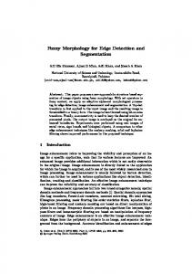
(a) Annotated cl map (coronal section)
(b) AO measure from [3]
7
(c) Sharper AO measure involving ∇cbp
Fig. 2. Extending the invariant gradients framework towards the Westin metrics allows for a sharper version of the adjacent orthogonality (AO) measure.
gradient from Equation (7), and a third vector which is the cross product of the first two and captures any remaining changes in shape. The fiber tracts in Figure 2 (a) are superior longitudinal fasciculus (slf), internal capsule (ic), corpus callosum (cc), cingulum (cing), and fornix (fx). Figure 2 (b) presents a map of the adjacent orthogonality (AO) measure, defined in [3] from the coordinates of the tensor field derivative in the invariant gradients c3 |2 )1/2 . It separates differently oriented tracts, c3 |2 +|∇φ framework as AO = (|∇R c3 , and rotations based on shape changes towards planarity, measured by ∇R c3 . For detailed information on rotation tangents Φ ci , around e3 , measured by ∇φ which are used to analyze changes in orientation, the reader is referred to [3]. For the task of separating differently oriented tracts, we select a basis of S that has ∇S cp as one of its axes. Since cp reacts more specifically to changes in planarity than R3 does, a sharper version of AO is then obtained by replacing c3 with ∇cbp . In particular, this produces clear borders in some locations where ∇R the original formulation of AO indicates no or only very unsharp boundaries (marked by arrows in Figure 2 (c)). Overlaying them on a color coded direction map confirms that they correspond precisely to tract interfaces.
5
Edge Detection in the Log-Euclidean Framework
The fact that negative diffusivities do not have any physical meaning restricts diffusion tensors to the positive definite cone within Sym3 , which is closed under addition and multiplication by positive scalars. Arsigny et al. [7] point out that after taking the matrix logarithm, one may process diffusion tensors with arbitrary (even non-convex) operations without leaving the positive definite cone in the original space, because the inverse map, the matrix exponential, maps all real numbers back to positive values. The matrix logarithm log D of a diffusion tensor D is computed by performing its spectral decomposition (Equation (1)) and taking the logarithm of the eigenvalues. Within this framework, edge strength is measured as k∇ log Dk. We refer to this as the Log-Euclidean edge detector, in contrast to the standard Euclidean edge detector k∇Dk. To simplify computations, it has been suggested to evaluate log D at sample positions and to obtain an approximation of k∇ log Dk by taking
8
T. Schultz et al.
(a) k∇ log Dk via finite differences
(b) k∇ log Dk via chain rule
(c) same as (a), after tensor estimation as in [16]
Fig. 3. Approximating k∇ log Dk via finite differences of logarithms leads to artifacts near steep edges ((a) and (c)). They are avoided by using the chain rule instead (b).
finite differences between the resulting matrices [7]. However, as we have seen in Figure 1 (c), approximating the derivative of a nonlinear function via finite differences may not produce sufficiently exact results. In fact, near steep edges like those between the ventricles (vent) and brain tissue, we observed artifacts in approximated edge maps of k∇ log Dk, marked by two arrows in Figure 3 (a). This problem can be avoided by applying the multivariate chain rule of differentiation, which is again simplified by considering eigenvalue derivatives. In the eigenframe of D, the Jacobian of the matrix logarithm log D takes on diagonal form: Let di,j be entry (i, j) of [D]E ¯ , li,j be the corresponding en−1 −1 try of [log D]E and for i 6= j, ∂li,j /∂di,j = ¯ . Then, ∂li,i /∂di,i = di,i = λi (log di,i − log dj,j )/(di,i − dj,j ). All other partial derivatives vanish. Thus, we −1 ′ simply obtain [(log D)′ ]E ¯ from [D ]E ¯ by multiplication of entries (i, i) by λi and multiplication of entries (i, j), i 6= j, by (log λi − log λj )/(λi − λj ). The resulting corrected map is shown in Figure 3 (b). We confirmed that the artifacts in Figure 3 (a) are not caused by estimating the tensors via the standard least squares method [1] and clamping the rare negative eigenvalues to a small positive epsilon afterwards. They are still present when using the gradient descent approach from [16], which integrates the positive definiteness constraint into the estimation process itself (Figure 3 (c)). The reformulation of the invariant gradients framework in terms of eigenvalue space allows us to apply it to Log-Euclidean edge detection, simply by considering the natural logarithms of eigenvalues as the fundamental axes of tensor shape space. Similar to the Euclidean case, the cylindrical coordinate system from [14] can be used to separate meaningful types of edges. Figure 4 (a) shows edges in overall diffusivity, Figure 4 (b) edges in anisotropy. In both cases, the Euclidean result is on the left, the Log-Euclidean one on the right. The Log-Euclidean approach measures overall diffusivity by the matrix determinant instead of the trace. The determinant also reflects eigenvalue dispersion, which explains why the contours of some fiber tracts appear in the right image of Figure 4 (a). In the Euclidean case, they are isolated more cleanly in the anisotropy channel. Consequently, anisotropy contours appear more blurred in the Log-Euclidean case. Overlaying them on a principal eigenvector color map indicates that they are offset towards the inside of fiber tracts in some places
Using Eigenvalue Derivatives for Edge Detection in DT-MRI Data
(a) Changes in overall diffusivity
9
(b) Changes in anisotropy
Fig. 4. Different types of edges are distinguished more cleanly by a Euclidean (left sub-images) than by a Log-Euclidean edge detector (right sub-images).
(arrows in Figure 4 (b)). Maps of the third shape axis, which captures transitions between linearity and planarity, were extremely similar (not shown).
6
Conclusion
Given the ubiquity of the spectral decomposition in DT-MRI processing, eigenvalue derivatives are a natural candidate for the analysis of local changes in this kind of data. In the present work, we have used them to generate edge maps with respect to the widely used Westin shape metrics [12], which we have shown to identify anatomical interfaces in real DT-MRI data and to allow for a more specific analysis of changes in tensor shape than has been possible with previously suggested edge detectors. The existing edge detection framework based on invariant gradients [3] is both simplified and easily extended by considering it in terms of eigenvalue derivatives. Finally, we have applied our results to analyze the relatively recent Log-Euclidean edge detector [7]. We have both corrected a source of artifacts in its previously proposed form and demonstrated that it, too, allows for separation of different types of edges, yet with a slightly lower anatomical specificity than the more traditional Euclidean detector.
Acknowledgements We would like to thank Bernhard Burgeth, who is with the Mathematical Image Analysis group at Saarland University, Germany, for in-depth discussions and for proofreading our manuscript. We are grateful to Alfred Anwander, who is with the Max Planck Institute for Human Cognitive and Brain Science in Leipzig, Germany, for providing the dataset and helping with the annotations. We thank Gordon Kindlmann, who is with the Laboratory of Mathematics in Imaging, Harvard Medical School, for providing the teem libraries (http://teem.sf.net/) and giving feedback on our results. This work has partially been funded by the Max Planck Center for Visual Computing and Communication (MPC-VCC).
10
T. Schultz et al.
References 1. Basser, P.J., Mattiello, J., Bihan, D.L.: Estimation of the effective self-diffusion tensor from the NMR spin echo. Journal of Magnetic Resonance B(103) (1994) 247–254 2. Pajevic, S., Aldroubi, A., Basser, P.J.: A continuous tensor field approximation of discrete DT-MRI data for extracting microstructural and architectural features of tissue. Journal of Magnetic Resonance 154 (2002) 85–100 3. Kindlmann, G., Ennis, D., Whitaker, R., Westin, C.F.: Diffusion tensor analysis with invariant gradients and rotation tangents. IEEE Transactions on Medical Imaging 26(11) (2007) 1483–1499 4. Kindlmann, G.: Visualization and Analysis of Diffusion Tensor Fields. PhD thesis, School of Computing, University of Utah (September 2004) 5. Schultz, T., Burgeth, B., Weickert, J.: Flexible segmentation and smoothing of DT-MRI fields through a customizable structure tensor. In Bebis, G., Boyle, R., Parvin, B., Koracin, D., Remagnino, P., Nefian, A.V., Gopi, M., Pascucci, V., Zara, J., Molineros, J., Theisel, H., Malzbender, T., eds.: Advances in Visual Computing. Volume 4291 of Lecture Notes in Computer Science., Springer (2006) 455–464 6. Kato, T.: Perturbation theory for linear operators. 2nd edn. Volume 132 of Die Grundlehren der mathematischen Wissenschaften. Springer (1976) 7. Arsigny, V., Fillard, P., Pennec, X., Ayache, N.: Log-euclidean metrics for fast and simple calculus on diffusion tensors. Magnetic Resonance in Medicine 56(2) (2006) 411–421 8. Anderson, A.W.: Theoretical analysis of the effects of noise on diffusion tensor imaging. Magnetic Resonance in Medicine 46(6) (2001) 1174–1188 9. O’Donnell, L., Grimson, W.E.L., Westin, C.F.: Interface detection in diffusion tensor MRI. In Barillot, C., Haynor, D., Hellier, P., eds.: Medical Image Computing and Computer-Assisted Intervention (MICCAI ’04). Volume 3216 of LNCS., Springer (2004) 360–367 10. Kindlmann, G., Tricoche, X., Westin, C.F.: Delineating white matter structure in diffusion tensor MRI with anisotropy creases. Medical Image Analysis 11(5) (2007) 492–502 11. Basser, P.J., Pierpaoli, C.: Microstructural and physiological features of tissues elucidated by quantitative-diffusion-tensor MRI. Journal of Magnetic Resonance B(111) (1996) 209–219 12. Westin, C.F., Peled, S., Gudbjartsson, H., Kikinis, R., Jolesz, F.A.: Geometrical diffusion measures for MRI from tensor basis analysis. In: International Society for Magnetic Resonance in Medicine ’97, Vancouver, Canada (1997) 1742 13. Pajevic, S., Pierpaoli, C.: Color schemes to represent the orientation of anisotropic tissues from diffusion tensor data: application to white matter fiber tract mapping in the human brain. Magnetic Resonance in Medicine 42(3) (1999) 526–540 14. Bahn, M.M.: Invariant and orthonormal scalar measures derived from magnetic resonance diffusion tensor imaging. Journal of Magnetic Resonance 141 (1999) 68–77 15. Ennis, D.B., Kindlmann, G.: Orthogonal tensor invariants and the analysis of diffusion tensor magnetic resonance images. Magnetic Resonance in Medicine 55(1) (2006) 136–146 16. Fillard, P., Pennec, X., Arsigny, V., Ayache, N.: Clinical DT-MRI estimation, smoothing and fiber tracking with log-euclidean metrics. IEEE Transactions on Medical Imaging 26(11) (2007) 1472–1482