Using Imbalance Metrics to Optimize Task Clustering in ... - SciTech

Using Imbalance Metrics to Optimize Task Clustering in Scientific Workflow Executions Weiwei Chena,∗, Rafael Ferreira da Silvaa , Ewa Deelmana , Rizos Sakellarioub a University

of Southern California, Information Sciences Institute, Marina del Rey, CA, USA of Manchester, School of Computer Science, Manchester, U.K.

b University

Abstract Scientific workflows can be composed of many fine computational granularity tasks. The runtime of these tasks may be shorter than the duration of system overheads, for example, when using multiple resources of a cloud infrastructure. Task clustering is a runtime optimization technique that merges multiple short running tasks into a single job such that the scheduling overhead is reduced and the overall runtime performance is improved. However, existing task clustering strategies only provide a coarse-grained approach that relies on an over-simplified workflow model. In this work, we examine the reasons that cause Runtime Imbalance and Dependency Imbalance in task clustering. Then, we propose quantitative metrics to evaluate the severity of the two imbalance problems. Furthermore, we propose a series of task balancing methods (horizontal and vertical) to address the load balance problem when performing task clustering for five widely used scientific workflows. Finally, we analyze the relationship between these metric values and the performance of proposed task balancing methods. A trace-based simulation shows that our methods can significantly decrease the runtime of workflow applications when compared to a baseline execution. We also compare the performance of our methods with two algorithms described in the literature. Keywords: Scientific workflows, Performance analysis, Scheduling, Workflow simulation, Task clustering, Load balancing

1. Introduction Many computational scientists develop and use large-scale, loosely-coupled applications that are often structured as scientific workflows. Although the majority of the tasks within these applications are often relatively short running (from a few seconds to a few minutes), in aggregate they represent a significant amount of computation and data [1, 3]. When executing these applications in a multi-machine, distributed environment, such as the Grid or the Cloud, significant system overheads may exist and may slowdown the application execution [4]. To reduce the impact of such overheads, task clustering techniques [5, 6, 7, 8, 9, 10, 11, 12, 13] have been developed to group fine-grained tasks into coarse-grained tasks so that the number of computational activities is reduced and so that their computational granularity is increased. This reduced the (mostly scheduling related) system overheads. However, there are several challenges that have not yet been addressed. A scientific workflow is typically represented as a directed acyclic graph (DAG). The nodes represent computations and the edges describe data and control dependencies between them. Tasks within a level (or depth within a workflow DAG) may have different runtimes. Proposed task clustering techniques that merge tasks within a level without considering the runtime variance may cause load imbalance, i.e., some clus∗ Corresponding

address: USC Information Sciences Institute, 4676 Admiralty Way Ste 1001, Marina del Rey, CA, USA, 90292, Tel: +1 310 448-8408 Email addresses: [email protected] (Weiwei Chen), [email protected] (Rafael Ferreira da Silva), [email protected] (Ewa Deelman), [email protected] (Rizos Sakellariou) Preprint submitted to Future Generation of Computer Systems

tered jobs may be composed of short running tasks while others of long running tasks. This imbalance delays the release of tasks from the next level of the workflow, penalizing the workflow execution with an overhead produced by the use of inappropriate task clustering strategies [14]. A common technique to handle load imbalance is overdecomposition [15]. This method decomposes computational work into mediumgrained balanced tasks. Each task is coarse-grained enough to enable efficient execution and reduce scheduling overheads, while being fine-grained enough to expose significantly higher application-level parallelism than what is offered by the hardware. Data dependencies between workflow tasks play an important role when clustering tasks within a level. A data dependency means that there is a data transfer between two tasks (output data for one and input data for the other). Grouping tasks without considering these dependencies may lead to data locality problems, where output data produced by parent tasks are poorly distributed. As a result, data transfer times and failure probabilities increase. Therefore, we claim that data dependencies of subsequent tasks should be considered. We generalize these two challenges (Runtime Imbalance and Dependency Imbalance) to the general task clustering load balance problem. We introduce a series of balancing methods to address these challenges. However, there is a tradeoff between runtime and data dependency balancing. For instance, balancing runtime may aggravate the Dependency Imbalance problem, and vice versa. Therefore, we propose a series of quantitative metrics that reflect the internal structure (in terms of task runtimes and dependencies) of the workflow and use them as a September 11, 2014

criterion to select and balance the solutions. In particular, we provide a novel approach to capture the imbalance metrics. Traditionally, there are two approaches to improve the performance of task clustering. The first one is a topdown approach [16] that represents the clustering problem as a global optimization problem and aims to minimize the overall workflow execution time. However, the complexity of solving such an optimization problem does not scale well since most solutions are based on genetic algorithms. The second one is a bottom-up approach [5, 11] that only examines free tasks to be merged and optimizes the clustering results locally. In contrast, our work extends these approaches to consider the neighboring tasks including siblings, parents, and children, because such a family of tasks has strong connections between them. The quantitative metrics and balancing methods were introduced and evaluated in [17] on five workflows. In this paper, we extend this previous work by studying: • the performance gain of using our balancing methods over a baseline execution on a larger set of workflows; • the performance gain over two additional task clustering methods described in the literature [10, 11]; • the performance impact of the variation of the average data size and number of resources; • the performance impact of combining our balancing methods with vertical clustering. The rest of the paper is organized as follows. Section 2 gives an overview of the related work. Section 3 presents our workflow and execution environment models. Section 4 details our heuristics and algorithms for balancing. Section 5 reports experiments and results, and the paper closes with a discussion and conclusions.

and Cloud systems. Several works have addressed the control of task granularity of bags of tasks. For instance, Muthuvelu et al. [5] proposed a clustering algorithm that groups bags of tasks based on their runtime—tasks are grouped up to the resource capacity. Later, they extended their work [6] to determine task granularity based on task file size, CPU time, and resource constraints. Recently, they proposed an online scheduling algorithm [7, 8] that groups tasks based on resource network utilization, user’s budget, and application deadline. Ng et al. [9] and Ang et al. [10] introduced bandwidth in the scheduling framework to enhance the performance of task scheduling. Longer tasks are assigned to resources with better bandwidth. Liu and Liao [11] proposed an adaptive fine-grained job scheduling algorithm to group fine-grained tasks according to processing capacity and bandwidth of the current available resources. Although these techniques significantly reduce the impact of scheduling and queuing time overhead, they do not consider data dependencies. Task granularity control has also been addressed in scientific workflows. For instance, Singh et al. [12] proposed leveland label-based clustering. In level-based clustering, tasks at the same level of the workflow can be clustered together. The number of clusters or tasks per cluster are specified by the user. In the label-based clustering method, the user labels tasks that should be clustered together. Although their work considers data dependencies between workflow levels, it is done manually by the users, which is prone to errors and it is not scalable. Recently, Ferreira da Silva et al. [13, 21] proposed task grouping and ungrouping algorithms to control workflow task granularity in a non-clairvoyant and online context, where none or few characteristics about the application or resources are known in advance. Their work significantly reduced scheduling and queuing time overheads, but did not consider data dependencies. A plethora of balanced scheduling algorithms have been developed in the networking and operating system domains. Many of these schedulers have been extended to the hierarchical setting. Lifflander et al. [15] proposed to use work stealing and a hierarchical persistence-based rebalancing algorithm to address the imbalance problem in scheduling. Zheng et al. [22] presented an automatic hierarchical load balancing method that overcomes the scalability challenges of centralized schemes and poor solutions of traditional distributed schemes. There are other scheduling algorithms [2] that indirectly achieve load balancing of workflows through makespan minimization. However, the benefit that can be achieved through traditional scheduling optimization is limited by its complexity. The performance gain of task clustering is primarily determined by the ratio between system overheads and task runtime, which is more substantial in modern distributed systems such as Clouds and Grids. Workflow patterns [26, 3, 27] are used to capture and abstract the common structure within a workflow and they give insights on designing new workflows and optimization methods. Yu and Buyya [26] proposed a taxonomy that characterizes and classifies various approaches for building and executing workflows on Grids. They also provided a survey of several representative

2. Related Work System overhead analysis [18, 19] is a topic of great interest in the distributed computing community. Stratan et al. [20] evaluate in a real-world environment Grid workflow engines including DAGMan/Condor and Karajan/Globus. Their methodology focuses on five system characteristics: overhead, raw performance, stability, scalability, and reliability. They point out that resource consumption in head nodes should not be ignored and that the main bottleneck in a busy system is often the head node. Prodan et al. [19] offered a complete Grid workflow overhead classification and a systematic measurement of overheads. In Chen et al. [4], we extended [19] by providing a measurement of major overheads imposed by workflow management systems and execution environments and analyzed how existing optimization techniques improve the workflow runtime by reducing or overlapping overheads. The prevalent existence of system overheads is an important reason why task clustering provides significant performance improvement for workflowbased applications. In this chapter, we aim to further improve the performance of task clustering under imbalanced load. The low performance of fine-grained tasks is a common problem in widely distributed platforms where the scheduling overhead and queuing times at resources are high, such as Grid 2

Grid workflow systems developed by various projects worldwide to demonstrate the comprehensiveness of the taxonomy. Juve et al. [3] provided a characterization of workflow from six scientific applications and obtained task-level performance metrics (I/O, CPU, and memory consumption). They also presented an execution profile for each workflow running at a typical scale and managed by the Pegasus workflow management system [28, 32, 25]. Liu et al. [27] proposed a novel pattern based time-series forecasting strategy which utilizes a periodical sampling plan to build representative duration series. We illustrate the relationship between the workflow patterns (asymmetric or symmetric workflows) and the performance of our balancing algorithms. Some work in the literature has further attempted to define and model workflow characteristics with quantitative metrics. In [29], the authors proposed a robustness metric for resource allocation in parallel and distributed systems and accordingly customized the definition of robustness. Tolosana et al. [30] defined a metric called Quality of Resilience to assess how resilient workflow enactment is likely to be in the presence of failures. Ma et al. [31] proposed a graph distance based metric for measuring the similarity between data oriented workflows with variable time constraints, where a formal structure called time dependency graph (TDG) is proposed and further used as representation model of workflows. Similarity comparison between two workflows can be reduced to computing the similarity between TDGs. In this work, we develop quantitative metrics to measure the severity of the imbalance problem in task clustering and then use the results to guide the selection of different task clustering methods.

Figure 1: A workflow system model.

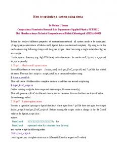
overheads are reduced (task clustering). A job is a single execution unit in the workflow execution systems and is composed of one or more tasks. Workflow Engine. Executes jobs defined by the workflow in order of their dependencies. Only jobs that have all their parent jobs completed are submitted to the Job Scheduler. The elapsed time from when a job is released (all of its parents have completed successfully) to when it is submitted to the job scheduler is denoted as the workflow engine delay. Job Scheduler and Local Queue. Manage individual workflow jobs and supervise their execution on local and remote resources. The scheduler relies on the resources (compute, storage, and network) defined in the executable workflow to perform computations. The elapsed time from when a task is submitted to the job scheduler to when it starts its execution in a worker node is denoted as the queue delay. It reflects both the efficiency of the job scheduler and resource availability.

3. Model and Design

Job Wrapper. Extracts tasks from clustered jobs and executes them at the worker nodes. The clustering delay is the elapsed time of the extraction process.

A workflow is modeled as a directed acyclic graph (DAG), where each node in the DAG often represents a workflow task (t), and the edges represent dependencies between the tasks that constrain the order in which tasks are executed. Dependencies typically represent data-flow dependencies in the application, where the output files produced by one task are used as inputs of another task. Each task is a computational program and a set of parameters that need to be executed. This model fits several workflow management systems such as Pegasus [32], Askalon [33], Taverna [34] and Galaxy [23]. In this paper, we assume that there is only one execution site with multiple compute resources, such as virtual machines on the clouds. Figure 1 shows a typical workflow execution environment. The submit host prepares a workflow for execution (clustering, mapping, etc.), and worker nodes, at an execution site, execute jobs individually. The main components are introduced below:

Figure 2: Extending DAG to o-DAG (s denotes a system overhead).

Workflow Mapper. Generates an executable workflow based on an abstract workflow [28] provided by the user or workflow composition system. It also restructures the workflow to optimize performance and adds tasks for data management and provenance information generation. The Workflow Mapper also merges small tasks together into a job such that system

We extend the DAG model to be overhead aware (o-DAG). System overheads play an important role in workflow execution and constitute a major part of the overall runtime when tasks are poorly clustered [4]. Figure 2 shows how we augment 3

a DAG to be an o-DAG with the capability to represent system overheads (s) such as workflow engine and queue delays. In addition, system overheads also include data transfer delays caused by staging-in and staging-out data. This classification of system overheads is based on our prior study on workflow analysis [4]. With an o-DAG model, we can explicitly express the process of task clustering. In this paper, we address horizontal and vertical task clustering. Horizontal Clustering (HC) merges multiple tasks that are at the same horizontal level of the workflow, in which the horizontal level of a task is defined as the longest distance from the entry task(s) of the DAG to this task (an entry task has no parents). Vertical Clustering (VC) merges tasks within a pipeline of the workflow. Tasks in the same pipeline share a single-parent-single-child relationship, which means a task ta is the unique parent of a task tb , which is the unique child of ta . Figure 3 shows a simple example of how to perform HC, in which two tasks t2 and t3 , without a data dependency between them, are merged into a clustered job j1 . A job j is a single execution unit composed by one or multiple task(s). Job wrappers are commonly used to execute clustered jobs, but they add an overhead denoted by the clustering delay c. The clustering delay measures the difference between the sum of the actual task runtimes and the job runtime seen by the job scheduler. After horizontal clustering, t2 and t3 in j1 can be executed in sequence or in parallel, if parallelism on one compute node is supported. In this paper, we consider sequential executions only. Given a single resource, the overall runtime for the P workflow in Figure 3 (left) is runtimel = 4i=1 (si + ti ), and the overall runtime for the clustered workflow in Figure 3 (right) is runtimer = s1 +t1 + s2 +c1 +t2 +t3 + s4 +t4 . runtimel > runtimer as long as c1 < s3 , which is the case in many distributed systems since the clustering delay within a single execution node is usually shorter than the scheduling overhead across different execution nodes.

Figure 4: An example of vertical clustering.

4. Balanced Clustering Task clustering has been widely used to address the low performance of very short running tasks on platforms where the system overhead is high, such as distributed computing infrastructures. However, up to now, techniques do not consider the load balance problem. In particular, merging tasks within a workflow level without considering the runtime variance may cause load imbalance (Runtime Imbalance), or merging tasks without considering their data dependencies may lead to data locality problems (Dependency Imbalance). In this section, we introduce metrics that quantitatively capture workflow characteristics to measure runtime and dependence imbalances. We then present methods to handle the load balance problem. 4.1. Imbalance metrics Runtime Imbalance describes the difference of the task/job runtime of a group of tasks/jobs. In this work, we denote the Horizontal Runtime Variance (HRV) as the ratio of the standard deviation in task runtime to the average runtime of tasks/jobs at the same horizontal level of a workflow. At the same horizontal level, the job with the longest runtime often controls the release of the next level jobs. A high HRV value means that the release of next level jobs has been delayed. Therefore, to improve runtime performance, it makes sense to reduce the standard deviation of job runtime. Figure 5 shows an example of four independent tasks t1 , t2 , t3 and t4 where the task runtime of t1 and t2 is 10 seconds, and the task runtime of t3 and t4 is 30 seconds. In the Horizontal Clustering (HC) approach, a possible clustering result could be to merge t1 and t2 into a clustered job, and t3 and t4 into another. This approach results in imbalanced runtime, i.e., HRV > 0 (Figure 5-top). In contrast, a balanced clustering strategy should try its best to evenly distribute task runtime among jobs as shown in Figure 5 (bottom). A smaller HRV means that the runtime of tasks within a horizontal level is more evenly distributed and

Figure 3: An example of horizontal clustering (color indicates the horizontal level of a task).

Figure 4 illustrates an example of vertical clustering, in which tasks t2 , t4 , and t6 are merged into j1 , while tasks t3 , t5 , and t7 are merged into j2 . Similarly, clustering delays c2 and c3 are added to j1 and j2 respectively, but system overheads s4 , s5 , s6 , and s7 are removed. 4

(IF) of a task tu is defined as follows:

therefore it is less necessary to use runtime-based balancing algorithms. However, runtime variance is not able to capture how symmetric the structure of the dependencies between tasks is.

IF(tu ) =

X tv ∈Child(tu

IF(tv ) ||Parent(t v )|| )

(1)

where Child(tu ) denotes the set of child tasks of tu , and ||Parent(tv )|| the number of parent tasks of tv . The Impact Factor aims to capture the similarity of tasks/jobs in a graph by measuring their relative impact factor or importance to the entire graph. Tasks with similar impact factors are merged together, so that the workflow structure tends to be more “even” or symmetric. For simplicity, we assume the IF of a workflow exit task (a task without children, e.g. t5 in Figure 6) is 1.0. Consider the two workflows presented in Figure 7. The IF for each of t1 , t2 , t3 , and t4 is computed as follows: IF(t7 ) = 1.0, IF(t6 ) = IF(t5 ) = IF(t7 )/2 = 0.5 IF(t1 ) = IF(t2 ) = IF(t5 )/2 = 0.25

Figure 5: An example of Horizontal Runtime Variance.

IF(t3 ) = IF(t4 ) = IF(t6 )/2 = 0.25 Thus, IFV(t1 , t2 , t3 , t4 ) = 0. In contrast, the IF for t10 , t20 , t30 , and t40 is:

Dependency Imbalance means that the task clustering at one horizontal level forces the tasks at the next level (or even subsequent levels) to have severe data locality problems and thus loss of parallelism. For example, in Figure 6, we show a two-level workflow composed of four tasks in the first level and two in the second. Merging t1 with t3 and t2 with t4 (imbalanced workflow in Figure 6) forces t5 and t6 to transfer files from two locations and wait for the completion of t1 , t2 , t3 , and t4 . A balanced clustering strategy groups tasks that have the maximum number of child tasks in common. Thus, t5 can start to execute as soon as t1 and t2 are completed, and so can t6 . To quantitatively measure the Dependency Imbalance of a workflow, we propose two metrics: (i) Impact Factor Variance, and (ii) Distance Variance.

IF(t70 ) = 1.0, IF(t60 ) = IF(t50 ) = IF(t10 ) = IF(t70 )/2 = 0.5 IF(t20 ) = IF(t30 ) = IF(t40 ) = IF(t60 )/3 = 0.17 Therefore, the IFV value for t10 , t20 , t30 , t40 is 0.17, which predicts that it is likely to be less symmetric than the workflow in Figure 7 (left). In this paper, we use HIFV (Horizontal IFV) to indicate the IFV of tasks at the same horizontal level. The time complexity of calculating the IF of all the tasks of a workflow with n tasks is O(n).

Figure 7: Example of workflows with different data dependencies (For better visualization, we do not show system overheads in the rest of the paper).

Distance Variance (DV) describes how ‘close’ tasks are to each other. The distance between two tasks/jobs is defined as the sum of the distance to their closest common successor. If they do not have a common successor, the distance is set to infinity. For a group of n tasks/jobs, the distance between them is represented by a n × n matrix D, where an element D(u, v) denotes the distance between a pair of tasks/jobs u and v. For any workflow structure, D(u, v) = D(v, u) and D(u, u) = 0, thus we ignore the cases when u ≥ v. Distance Variance is then defined as the standard deviation of all the elements D(u, v) for u < v. The time complexity of calculating all the values of D of a workflow with n tasks is O(n2 ). Similarly, HDV indicates the DV of a group of tasks/jobs at the same horizontal level. For example, Table 1 shows the distance matrices of tasks from the first level for both workflows

Figure 6: An example of Dependency Imbalance.

We define the Impact Factor Variance (IFV) of tasks as the standard deviation of their impact factors. The Impact Factor 5

of Figure 7 (D1 for the workflow in the left, and D2 for the workflow in the right). HDV for t1 , t2 , t3 , and t4 is 1.03, and for t10 , t20 , t30 , and t40 is 1.10. In terms of distance variance, D1 is more “even” than D2 . A smaller HDV means the tasks at the same horizontal level are more equally “distant” from each other and thus the workflow structure tends to be more “even” and symmetric. D1 t1 t2 t3 t4

t1 0 2 4 4

t2 2 0 4 4

t3 4 4 0 2

t4 4 4 2 0

D2 t10 t20 t30 t40

t10 0 4 4 4

t20 4 0 2 2

t30 4 2 0 2

highest runtime to the group with the shortest aggregated runtime. Thus, t1 and t3 , as well as t2 and t4 are merged together. For simplicity, system overheads are not displayed.

t40 4 2 2 0 Figure 8: An example of the HRB (Horizontal Runtime Balancing) method. By solely addressing runtime variance, data locality problems may arise.

Table 1: Distance matrices of tasks from the first level of workflows in Figure 7.

In conclusion, runtime variance and dependency variance offer a quantitative and comparable tool to measure and evaluate the internal structure of a workflow.

Algorithm 2 Horizontal Impact Factor Balancing algorithm. Require: W: workflow; R: number of jobs per horizontal level 1: procedure Clustering(W, R) 2: for level < depth(W) do 3: T L ← GetTasksAtLevel(W, level) . Partition W based on depth 4: C ← T L.size()/R . C is number of tasks per job in this level 5: CL ← Merge(T L, C, R) . Returns a list of clustered jobs 6: W ← W − T L + CL . Merge dependencies as well 7: end for 8: end procedure 9: procedure Merge(T L, C, R) 10: for i < R do 11: Ji ←{} . An empty job 12: end for 13: CL ←{} . An empty list of clustered jobs 14: Sort T L in descending of runtime 15: for all t in T L do 16: L ← Sort all Ji with the similarity of impact factors with t 17: J ← the job with shortest runtime and less than C tasks in L 18: J.add (t) 19: end for 20: for i < R do 21: CL.add( Ji ) 22: end for 23: return CL 24: end procedure

4.2. Balanced clustering methods In this subsection, we introduce our balanced clustering methods used to improve the runtime and dependency balances in task clustering. We first present the basic runtime-based clustering method, and then two other balancing methods that address the dependency imbalance problem. Algorithm 1 Horizontal Runtime Balancing algorithm. Require: W: workflow; R: number of jobs per horizontal level 1: procedure Clustering(W, R) 2: for level < depth(W) do 3: T L ← GetTasksAtLevel(W, level) . Partition W based on depth 4: C ← T L.size()/R . C is number of tasks per job in this level 5: CL ← Merge(T L, C, R) . Returns a list of clustered jobs 6: W ← W − T L + CL . Merge dependencies as well 7: end for 8: end procedure 9: procedure Merge(T L, C, R) 10: for i < R do 11: Ji ←{} . An empty job 12: end for 13: CL ←{} . An empty list of clustered jobs 14: Sort T L in descending of runtime 15: for all t in T L do 16: J ← the job with shortest runtime and less than C tasks 17: J.add (t) . Adds the task to the shortest job 18: end for 19: for i < R do 20: CL.add( Ji ) 21: end for 22: return CL 23: end procedure

However, HRB may cause a dependency imbalance problem since the clustering does not take data dependency into consideration. To address this problem, we propose the Horizontal Impact Factor Balancing (HIFB) and the Horizontal Distance Balancing (HDB) methods. In HRB, candidate jobs within a workflow level are sorted by their runtime, while in HIFB jobs are first sorted based on their similarity of IF, then based on runtime. Algorithm 2 shows the pseudocode of HIFB. For example, in Figure 9, t1 and t2 have IF = 0.25, while t3 , t4 , and t5 have IF = 0.16. HIFB selects a list of candidate jobs with the same IF value, and then HRB is performed to select the shortest job. Thus, HIFB merges t1 and t2 together, as well as t3 and t4 . However, HIFB is often suitable for workflows with an asymmetric structure. A symmetric workflow structure means there exists a (usually vertical) division of the workflow graph such that one part of the workflow is a mirror of the other part. For symmetric workflows, such as the one shown in Figure 8, the IF value for all tasks of the first level will be the same

Horizontal Runtime Balancing (HRB) aims to evenly distribute task runtime among clustered jobs. Tasks with the longest runtime are added to the job with the shortest runtime. Algorithm 1 shows the pseudocode of HRB. This greedy method is used to address the load balance problem caused by runtime variance at the same horizontal level. Figure 8 shows an example of HRB where tasks in the first level have different runtimes and should be grouped into two jobs. HRB sorts tasks in decreasing order of runtime, and then adds the task with the 6

Algorithm 3 Horizontal Distance Balancing algorithm.

There are cases where HDB would yield lower performance than HIFB. For instance, let t1 , t2 , t3 , t4 , and t5 be the set of tasks to be merged in the workflow presented in Figure 11. HDB does not identify the difference in the number of parent/child tasks between the tasks, since d(tu , tv ) = 2, ∀u, v ∈ [1, 5], u , v. On the other hand, HIFB does distinguish between them since their impact factors are slightly different. Example of such scientific workflows include the LIGO Inspiral workflow [35], which is used in the evaluation of this paper (Section 5.4).

Require: W: workflow; R: number of jobs per horizontal level 1: procedure Clustering(W, C) 2: for level < depth(W) do 3: T L ← GetTasksAtLevel(W, level) . Partition W based on depth 4: C ← T L.size()/R . C is number of tasks per job in this level 5: CL ← Merge(T L, C, R) . Returns a list of clustered jobs 6: W ← W − T L + CL . Merge dependencies as well 7: end for 8: end procedure 9: procedure Merge(T L, C, R) 10: for i < R do 11: Ji ←{} . An empty job 12: end for 13: CL ←{} . An empty list of clustered jobs 14: Sort T L in descending of runtime 15: for all t in T L do 16: L ← Sort all Ji with the closest distance with t 17: J ← the job with shortest runtime and less than C tasks in L 18: J.add (t) 19: end for 20: for i < R do 21: CL.add( Ji ) 22: end for 23: return CL 24: end procedure

Figure 11: A workflow example where HDB yields lower performance than HIFB. HDB does not capture the difference in the number of parents/child tasks, since the distances between tasks (t1 , t2 , t3 , t4 , and t5 ) are the same.

Table 2 summarizes the imbalance metrics and balancing methods introduced in this section. These balancing methods have different preferences when selecting a candidate job to be merged. For instance, HIFB tends to group tasks that share similar importance to the workflow structure, while HDB tends to group tasks that reduce data transfers.

Figure 9: An example of the HIFB (Horizontal Impact Factor Balancing) method. Impact factors allow the detection of similarities between tasks.

Imbalance Metrics Horizontal Runtime Variance Horizontal Impact Factor Variance Horizontal Distance Variance Balancing Methods Horizontal Runtime Balancing Horizontal Impact Factor Balancing Horizontal Distance Balancing

(IF = 0.25), thus the method may also cause dependency imbalance. In HDB, jobs are sorted based on the distance between them and the targeted task t, then on their runtimes. Algorithm 3 shows the pseudocode of HDB. For instance, in Figure 10, the distances between tasks D(t1 , t2 ) = D(t3 , t4 ) = 2, while D(t1 , t3 ) = D(t1 , t4 ) = D(t2 , t3 ) = D(t2 , t4 ) = 4. Thus, HDB merges a list of candidate tasks with the minimal distance (t1 and t2 , and t3 and t4 ). Note that even if the workflow is asymmetric (Figure 9), HDB would obtain the same result as with HIFB.

abbr. HRV HIFV HDV abbr. HRB HIFB HDB

Table 2: Summary of imbalance metrics and balancing methods.

4.3. Combining vertical clustering methods In this subsection, we discuss how we combine the balanced clustering methods presented above with vertical clustering (VC). In pipelined workflows (single-parent-single-child tasks), vertical clustering always yields improvement over a baseline, non-clustered execution because merging reduces system overheads and data transfers within the pipeline. Horizontal clustering does not have the same guarantee since its performance depends on the comparison of system overheads and task durations. However, vertical clustering has a limited performance improvement if the workflow does not have pipelines. Therefore, we are interested in the analysis of the performance impact of applying both vertical and horizontal clustering in

Figure 10: An example of the HDB (Horizontal Distance Balancing) method. Measuring the distances between tasks avoids data locality problems.

7

the same workflow. We combine these methods in two ways: (i) VC-prior, and (ii) VC-posterior.

5.1. Scientific workflow applications Five real scientific workflow applications are used in the experiments: LIGO Inspiral analysis [35], Montage [36], CyberShake [37], Epigenomics [38], and SIPHT [39]. In this subsection, we describe each workflow application and present their main characteristics and structures.

VC-prior. In this method, vertical clustering is performed first, and then the balancing methods (HRB, HIFB, HDB, or HC) are applied. Figure 12 shows an example where pipelined-tasks are merged first, and then the merged pipelines are horizontally clustered based on the runtime variance.

LIGO. Laser Interferometer Gravitational Wave Observatory (LIGO) [35] workflows are used to search for gravitational wave signatures in data collected by large-scale interferometers. The observatories’ mission is to detect and measure gravitational waves predicted by general relativity (Einstein’s theory of gravity), in which gravity is described as due to the curvature of the fabric of time and space. The LIGO Inspiral workflow is a data-intensive workflow. Figure 14 shows a simplified version of this workflow. The LIGO Inspiral workflow is separated into multiple groups of interconnected tasks, which we call branches in the rest of our paper. However, each branch may have a different number of pipelines as shown in Figure 14.

Figure 12: VC-prior: vertical clustering is performed first, and then the balancing methods.

Figure 14: A simplified visualization of the LIGO Inspiral workflow. Figure 13: VC-posterior: horizontal clustering (balancing methods) is performed first, and then vertical clustering (but without changes).

Montage. Montage [36] is an astronomy application that is used to construct large image mosaics of the sky. Input images are reprojected onto a sphere and overlap is calculated for each input image. The application re-projects input images to the correct orientation while keeping background emission level constant in all images. The images are added by rectifying them to a common flux scale and background level. Finally, the reprojected images are co-added into a final mosaic. The resulting mosaic image can provide a much deeper and detailed understanding of the portion of the sky in question. Figure 15 illustrates a small Montage workflow. The size of the workflow depends on the number of images used in constructing the desired mosaic of the sky. The structure of the workflow changes to accommodate increases in the number of inputs, which corresponds to an increase in the number of computational tasks.

VC-posterior. Here, horizontal balancing methods are first applied, and then vertical clustering is performed. Figure 13 shows an example where tasks are horizontally clustered first based on the runtime variance, and then merged vertically. However, since the original pipeline structures have been broken by horizontal clustering, VC does not perform any changes to the workflow. 5. Evaluation The experiments presented hereafter evaluate the performance of our balancing methods when compared to an existing and effective task clustering strategy named Horizontal Clustering (HC) [12], which is widely used by workflow management systems such as Pegasus [28]. We also compare our methods with two heuristics described in literature: DFJS [5], and AFJS [11]. DFJS groups bags of tasks based on the task durations up to the resource capacity. AFJS is an extended version of DFJS that is an adaptive fine-grained job scheduling algorithm to group fine-grained tasks according to processing capacity of the current available resources and bandwidth between these resources.

Cybershake. CyberShake [37] is a seismology application that calculates Probabilistic Seismic Hazard curves for geographic sites in the Southern California region. It identifies all ruptures within 200km of the site of interest and converts rupture definition into multiple rupture variations with differing hypocenter locations and slip distributions. It then calculates synthetic seismograms for each rupture variance, and peak intensity measures are then extracted from these synthetics and combined with the original rupture probabilities to produce probabilistic 8

Figure 15: A simplified visualization of the Montage workflow. Figure 17: A simplified visualization of the Epigenomics workflow with multiple branches.

seismic hazard curves for the site. Figure 16 shows an illustration of the Cybershake workflow.

(Basic Local Alignment Search Tools) comparisons of the inter genetic regions of different replicons and the annotations of any sRNAs that are found. A simplified structure of the SIPHT workflow is shown in Figure 18.

Figure 16: A simplified visualization of the CyberShake workflow.

Figure 18: A simplified visualization of the SIPHT workflow.

Epigenomics. The Epigenomics workflow [38] is a dataparallel workflow. Initial data are acquired from the IlluminaSolexa Genetic Analyzer in the form of DNA sequence lanes. Each Solexa machine can generate multiple lanes of DNA sequences. These data are converted into a format that can be used by sequence mapping software. The mapping software can do one of two major tasks. It either maps short DNA reads from the sequence data onto a reference genome, or it takes all the short reads, treats them as small pieces in a puzzle and then tries to assemble an entire genome. In our experiments, the workflow maps DNA sequences to the correct locations in a reference Genome. This generates a map that displays the sequence density showing how many times a certain sequence expresses itself on a particular location on the reference genome. Epigenomics is a CPU-intensive application and its simplified structure is shown in Figure 17. Different to the LIGO Inspiral workflow, each branch in Epigenomics has exactly the same number of pipelines, which makes it more symmetric.

Workflow LIGO Montage CyberShake Epigenomics SIPHT

Number of Tasks 800 300 700 165 1000

Average Data Size 5 MB 3 MB 148 MB 355 MB 360 KB

Average Task Runtime 228s 11s 23s 2952s 180s

Table 3: Summary of the scientific workflows characteristics.

Table 3 shows the summary of the main workflows characteristics: number of tasks, average data size, and average task runtimes for the five workflows. More detailed characteristics could be found in [3]. 5.2. Task clustering techniques The experiments compare the performance of our balancing methods to the Horizontal Clustering (HC) [12] technique, and with two methods well known from the literature, DFJS [5] and AFJS [11]. In this subsection, we briefly describe each of these algorithms.

SIPHT. The SIPHT workflow [39] conducts a wide search for small untranslated RNAs (sRNAs) that regulates several processes such as secretion or virulence in bacteria. The kingdomwide prediction and annotation of sRNA encoding genes involves a variety of individual programs that are executed in the proper order using Pegasus [28]. These involve the prediction of ρ-independent transcriptional terminators, BLAST

HC. Horizontal Clustering (HC) merges multiple tasks that are at the same horizontal level of the workflow. The clustering 9

AFJS. The adaptive fine-grained job scheduler (AFJS) [11] is an extension of DFJS. It groups tasks not only based on the maximum runtime defined per cluster job, but also on the maximum data size per clustered job. The algorithm adds tasks to a clustered job until the job’s runtime is greater than the maximum runtime or the job’s total data size (input + output) is greater than the maximum data size. The AFJS heuristic pseudocode is shown in Algorithm 6.

granularity (number of tasks within a cluster) of a clustered job is controlled by the user, who defines either the number of tasks per clustered job (clusters.size), or the number of clustered jobs per horizontal level of the workflow (clusters.num). This algorithm has been implemented and used in Pegasus [12]. For simplicity, we define clusters.num as the number of available resources. In our prior work [17], we have compared the runtime performance with different clustering granularity. The pseudocode of the HC technique is shown in Algorithm 4.

Algorithm 6 AFJS algorithm. Algorithm 4 Horizontal Clustering algorithm.

Require: W: workflow; max.runtime: the maximum runtime for a clustered jobs; max.datasize: the maximum data size for a clustered job 1: procedure Clustering(W, max.runtime) 2: for level max.runtime OR J.datasize + t.datasize > max.datasize then 14: CL.add(J) 15: J ←{} 16: end if 17: J.add(t) 18: end while 19: return CL 20: end procedure

Require: W: workflow; C: max number of tasks per job defined by clusters.size or clusters.num 1: procedure Clustering(W, C) 2: for level < depth(W) do 3: T L ← GetTasksAtLevel(W, level) . Partition W based on depth 4: CL ← Merge(T L, C) . Returns a list of clustered jobs 5: W ← W − T L + CL . Merge dependencies as well 6: end for 7: end procedure 8: procedure Merge(T L, C) 9: J ← {} . An empty job 10: CL ←{} . An empty list of clustered jobs 11: while T L is not empty do 12: J.add (T L.pop(C) . Pops C tasks that are not merged 13: CL.add( J) 14: end while 15: return CL 16: end procedure

DFJS. The dynamic fine-grained job scheduler (DFJS) was proposed by Muthuvelu et al. [5]. The algorithm groups bags of tasks based on their granularity size—defined as the processing time of the task on the resource. Resources are ordered by their decreasing values of capacity (in MIPS), and tasks are grouped up to the resource capacity. This process continues until all tasks are grouped and assigned to resources. Algorithm 5 shows the pseudocode of the heuristic.

DFJS and AFJS require parameter tuning (e.g. maximum runtime per clustered job) to efficiently cluster tasks into coarsegrained jobs. For instance, if the maximum runtime is too high, all tasks may be grouped into a single job, leading to loss of parallelism. In contrast, if the runtime threshold is too low, the algorithms do not group tasks, leading to no improvement over a baseline execution. For comparison purposes, we performed a parameter study in order to tune the algorithms for each workflow application described in Section 5.1. Exploring all possible parameter combinations is a cumbersome and exhaustive task. In the original DFJS and AFJS works, these parameters are empirically chosen, however this approach requires deep knowledge of the workflow applications. Instead, we performed a parameter tuning study, where we first estimated the upper bound of max.runtime (n) as the sum of all task runtimes, and the lower bound of max.runtime (m) as 1 second for simplicity. Data points were divided into ten chunks and then we sample one data point from each chunk. We then selected the chunk that has the lowest makespan and set n and m as the upper and lower bounds of the selected chunk, respectively. These steps were repeated until n and m had converged into a data point. To demonstrate the correctness of our sampling approach in practice, we show the relationship between the makespan and the max.runtime for an example Montage workflow application in Figure 19—experiment conditions are presented in Sec-

Algorithm 5 DFJS algorithm. Require: W: workflow; max.runtime: max runtime of clustered jobs 1: procedure Clustering(W, max.runtime) 2: for level max.runtime then 14: CL.add(J) 15: J ←{} 16: end if 17: J.add(t) 18: end while 19: return CL 20: end procedure

10

tion 5.3. Data points are divided into 10 chunks of 250s each (for max.runtime). As the lower makespan values belongs to the first chunk, n is updated to 250, and m to 1. The process repeats until the convergence around max.runtime=180s. Even though there are multiple local minimal makespan values, these data points are close to each other, and the difference between their values (on the order of seconds) is negligible.

clustered jobs, which is a simple selection of granularity control of the strength of task clustering. The study of granularity size has been done in [17], which shows that such selection is acceptable. We collected workflow execution traces [3, 4] (including overhead and task runtime information) from real runs (executed on FutureGrid and Amazon EC2) of the scientific workflow applications described in Section 5.1. The traces are used as input to the Workflow Generator toolkit [47] to generate synthetic workflows. This allows us to perform simulations with several different application configurations under controlled conditions. The toolkit uses the information gathered from actual scientific workflow executions to generate synthetic workflows resembling those used by real world scientific applications. The number of inputs to be processed, the number of tasks in the workflow, and their composition determine the structure of the generated workflow. Such an approach of traced-based simulation allows us to utilize real traces and vary the system parameters (i.e., the number of VMs) and workflow (i.e., avg. data size) to fully explore the performance of our balanced task clustering algorithms. Three sets of experiments were conducted. Experiment 1 evaluated the performance gain (µ) of our balancing methods (HRB, HIFB, and HDB) over a baseline execution that had no task clustering. We define the performance gain (µ) over a baseline execution as the performance of the balancing methods related to the performance of an execution without clustering. Thus, for values of µ > 0 our balancing methods perform better than the baseline execution. Otherwise, the balancing methods perform poorer. The goal of the experiment is to identify conditions, where each method works best and worst. In addition, we also evaluate the performance gain of using workflow structure metrics (HRV, HIFV, and HDV), which require less a-priori knowledge about task and resource characteristics, than task clustering techniques in literature (HC, DFJS*, and AFJS*). Experiment 2 evaluates the performance impact of the variation of average data size (defined as the average of all the input and output data) and the number of resources available in our balancing methods for one scientific workflow application (LIGO). The original average data size (both input and output data) of the LIGO workflow is approximately 5MB as shown in Table 3. In this experiment, we increase the average data size up to 500MB to study the behavior of data-intensive workflows. We control resource contention by varying the number of available resources (VMs). High resource contention is achieved by setting the number of available VMs to 5, which represents fewer than 10% of the required resources to compute all tasks in parallel. On the other hand, low contention is achieved when the number of available VMs is increased to 25, which represents about 50% of the required resources. Experiment 3 evaluates the influence of combining our horizontal clustering methods with vertical clustering (VC). We compare the performance gain under four scenarios: (i) VCprior, VC is first performed and then HRB, HIFB, or HDB; (ii) VC-posterior, horizontal methods are performed first and then VC; (iii) No-VC, horizontal methods only; and (iv) VC-only, no

5000

Makespan(seconds)

4500 4000 3500 3000 2500 2000 1500 0

180

500

1000

1500

2000

2500

Max.runtime(seconds)

Figure 19: Relationship between the makespan of workflow and the specified maximum runtime in DFJS (Montage).

For simplicity, in the rest of this paper we use DFJS* and AFJS* to indicate the best estimated performance of DFJS and AFJS respectively using the sampling approach described above. 5.3. Experiment conditions We adopted a trace-based simulation approach, where we extended our WorkflowSim [40] simulator with the balanced clustering methods and imbalance metrics to simulate a controlled distributed execution environment. WorkflowSim is a workflow simulator that extends CloudSim [41] by providing support for task clustering, task scheduling, and resource provisioning at the workflow level. It has been recently used in multiple workflow studies [17, 42, 43] and its correctness has been verified in [40]. The simulated computing platform is composed by 20 single homogeneous core virtual machines (worker nodes), which is the quota per user of some typical distributed environments such as Amazon EC2 [44] and FutureGrid [45]. Amazon EC2 is a commercial, public cloud that has been widely used in distributed computing, in particular for scientific workflows [46]. FutureGrid is a distributed, high-performance testbed that provides scientists with a set of computing resources to develop parallel, grid, and cloud applications. Each simulated virtual machine (VM) has 512MB of memory and the capacity to process 1,000 million instructions per second. The default network bandwidth is 15MB per second according to the real environment in FutureGrid from, where our traces were collected. The task scheduling algorithm is data-aware, i.e. tasks are scheduled to resources, which have the most input data available. By default, we merge tasks at the same horizontal level into 20 11

horizontal methods. Table 4 shows the results of combining VC with horizontal methods. For example, VC-HIFB indicates we perform VC first and then HIFB.

50

40

30

HIFB VC-HIFB HIFB-VC VC HIFB

HDB VC-HDB HDB-VC VC HDB

HRB VC-HRB HRB-VC VC HRB

HC VC-HC HC-VC VC HC

µ%

Combination VC-prior VC-posterior VC-only No-VC

20

10

0 Cybershake

Table 4: Combination Results. ‘-’ indidates the order of performing these algorithms, i.e., VC-HIFB indicates we perform VC first and then HIFB.

Epigenomics

HRB

LIGO

HIFB

HDB

Montage

HC

DFJS*

SIPHT

AFJS*

Figure 20: Experiment 1: performance gain (µ) over a baseline execution for six algorithms (* indicates the tuned performance of DFJS and AFJS). By default, we have 20 VMs.

5.4. Results and discussion Experiment 1. Figure 20 shows the performance gain µ of the balancing methods for the five workflow applications over a baseline execution. All clustering techniques significantly improve (up to 48%) the runtime performance of all workflow applications, except HC for SIPHT. The reason is that SIPHT has a high HRV compared to other workflows as shown in Table 5. This indicates that the runtime imbalance problem in SIPHT is more significant and thus it is harder for HC to improve the workflow performance. Cybershake and Montage workflows have the highest gain, but nearly the same improvement independent of the algorithm. This is due to their symmetric structure and low values for the imbalance metrics and the distance metrics as shown in Table 5. Epigenomics and LIGO have a higher average task runtime and thus a lower performance gain. However, Epigenomices and LIGO have a higher variance of runtime and of distance and thus the performance improvement of HRB and HDB is better than that of HC, which is more significant compared to other workflows. In particular, each branch of the Epigenomics workflow (Figure 17) has the same number of pipelines, consequently the IF values of tasks in the same horizontal level are the same. Therefore, HIFB cannot distinguish tasks from different branches, which leads the system to a dependency imbalance problem. In such cases, HDB captures the dependency between tasks and yields better performance. Furthermore, Epigenomics and LIGO workflows have a high runtime variance, which has a higher impact on the performance than data dependency. Last, the performance gain of our balancing methods is in most cases better than the welltuned algorithms DFJS* and AFJS*. The other benefit is that our balancing methods do not require parameter tuning, which is cumbersome in practice.

the application’s performance. HIFB captures both the workflow structure and task runtime information, which reduces data transfers between tasks and consequently yields a better performance improvement over the baseline execution. HDB captures the strong connections between tasks (data dependencies), while HIFB captures the weak connections (similarity in terms of structure). In some cases, HIFV is zero while HDV is less likely to be zero. Most of the LIGO branches are like the ones in Figure 14, however, as mentioned in Section 4.2, the LIGO workflow has a few branches that depend on each other as shown in Figure 11. Since most branches are isolated from each other, HDB initially performs well compared to HIFB. However, as the average data size is increased, the performance of HDB is more and more constrained by the interdependent branches as shown in Figure 21. HC shows a nearly constant performance despite of the average data size, due to its random merging of tasks at the same horizontal level regardless of the runtime and data dependency information. 20

µ%

15

10

5

0 5 MB

Experiment 2. Figure 21 shows the performance gain µ of HRB, HIFB, HDB, and HC over a baseline execution for the LIGO Inspiral workflow. We chose LIGO because the performance improvement among these balancing methods is significantly different for LIGO compared to other workflows as shown in Figure 20. For small data sizes (up to 100 MB), the application is CPU-intensive and runtime variations have higher impact on the performance of the application. Thus, HRB performs better than any other balancing method. When increasing the average data size, the application turns into a data-intensive application, i.e. data dependencies have a higher impact on

50 MB

100 MB

HRB

250 MB

HIFB

HDB

400 MB

500 MB

HC

Figure 21: Experiment 2: performance gain (µ) over a baseline execution with different average data sizes for the LIGO workflow. The original avg. data size is 5MB.

Figures 22 and 23 show the performance gain µ when varying the number of available VMs for the LIGO workflows with an average data size of 5MB (CPU-intensive) and 500MB (dataintensive) respectively. In high contention scenarios (small number of available VMs), all methods perform similarly when 12

3 39 39 39 39 3 1 1 1 191 191 18 191 191 18 49 196 1 1 49 1 1 1 1 712 64 128 32 32 32

HDV

the high system overhead. Similarly to the CPU-intensive case, under low contention, runtime variance increases its importance and then HRB performs better.

1.22 0.00 26.20 0.00 0.00 578 421 264 107 0.00 0.00 0.00 0.00

20 µ%

4 347 348 1

HRV HIFV (a) CyberShake 0.309 0.03 0.282 0.00 0.397 0.00 0.000 0.00 (b) Epigenomics 0.327 0.00 0.393 0.00 0.328 0.00 0.358 0.00 0.290 0.00 0.247 0.00 0.000 0.00 0.000 0.00 0.000 0.00 (c) LIGO 0.024 0.01 0.279 0.01 0.054 0.00 0.066 0.01 0.271 0.01 0.040 0.00 (d) Montage 0.022 0.01 0.010 0.00 0.000 0.00 0.000 0.00 0.017 0.00 0.000 0.00 0.000 0.00 0.000 0.00 0.000 0.00 (e) SIPHT 3.356 0.01 1.078 0.01 1.719 0.00 0.000 0.00 0.210 0.00 0.000 0.00

10

0 5

10

15 Number of VMs HRB

10097 8264 174 5138 3306 43.70

HIFB

HDB

20

25

HC

Figure 22: Experiment 2: performance gain (µ) over baseline execution with different number of resources for the LIGO workflow (average data size is 5MB).

30

189.17 0.00 0.00 0.00 0.00 0.00 0.00 0.00 0.00

20 µ%

# of Tasks Level 1 2 3 4 Level 1 2 3 4 5 6 7 8 9 Level 1 2 3 4 5 6 Level 1 2 3 4 5 6 7 8 9 Level 1 2 3 4 5 6

10

0 5

53199 1196 3013 342 228 114

10

15 Number of VMs HRB

HIFB

HDB

20

25

HC

Figure 23: Experiment 2: performance gain (µ) over baseline execution with different number of resources for the LIGO workflow (average data size is 500MB).

Table 5: Experiment 1: average number of tasks, and average values of imbalance metrics (HRV, HIFV, and HDV) for the five workflow applications (before task clustering).

To evaluate the performance of our algorithms in a larger scale scenario, we increase the number of tasks in LIGO to 8,000 (following the same structure rules enforced by the WorkflowGenerator toolkit) and simulate the execution with [200, 1800] VMs. We choose 1,800 as the maximum number of VMs because the LIGO workflow has a maximum width of 1892 tasks (at the same level). Figure 24 shows the performance gain over the baseline execution with different numbers of resources for the LIGO workflow. In a small scale (i.e., 200 VMs), HRB and HDB perform slightly better than the other methods. However, as the scale increases, HDB outperforms the other methods. Similarly to the results obtained in Figure 23, HRB performs worse in larger scales since the runtime imbalance is no longer a major issue (HRV is too small) and thus the dependency imbalance becomes the bottleneck. Within the two dependency-oriented optimization methods, HDB outperforms HIFB since HDB captures the strong relation between tasks (distance), while HIFB uses the impact factor based metrics to capture the structural similarity.

the application is CPU-intensive (Figure 22), i.e., runtime variance and data dependency have a smaller impact than the system overhead (e.g. queuing time). As the number of available resources increases, and the data size is too small, runtime variance has more impact on the application’s performance, thus HRB performs better than the others. Note that as HDB captures strong connections between tasks, it is less sensitive to the runtime variations than HIFB, thus it yields better performance. For the data-intensive case (Figure 23), data dependencies have more impact on the performance than the runtime variation does. In particular, in the high contention scenario HDB performs poor clustering leading the system to data locality problems compared to HIFB due to the interdependent branches in the LIGO workflow. However, the method still improves the execution time of the workflow over the baseline case due to 13

50 60 40 40 µ%

µ%

30

20 20 10

0

0 200

400

600

800

1000 1200 Number of VMs

HRB

HIFB

HDB

1400

1600

HRB

1800

HIFB

VC−prior

HC

HDB

VC−posterior

HC

No−VC

VC−only

VC−only

Figure 26: Experiment 3: performance gain (µ) for the Montage workflow over baseline execution when using vertical clustering (VC).

Figure 24: Experiment 2: performance gain (µ) over baseline execution with different number of resources for the LIGO workflow (number of tasks is 8000).

Experiment 3. Figure 25 shows the performance gain µ for the Cybershake workflow over the baseline execution when using vertical clustering (VC) combined to our balancing methods. Vertical clustering does not show any improvement for the Cybershake workflow (µ(VC-only) ≈ 0.2%), because the workflow structure has no explicit pipelines (see Figure 16). Similarly, VC does not improve the SIPHT workflow due to the lack of pipelines in its structure (Figure 18). Thus, results for this workflow are omitted.

20

µ%

15

10

5

0 HRB

HIFB

VC−prior

HDB

VC−posterior

HC

No−VC

VC−only

VC−only

50

40

Figure 27: Experiment 3: performance gain (µ) for the LIGO workflow over baseline execution when using vertical clustering (VC).

µ%

30

20 20 10 15 0 HIFB

VC−prior

HDB

VC−posterior

HC

No−VC

VC−only

µ%

HRB

VC−only

10

5

0

Figure 25: Experiment 3: performance gain (µ) for the Cybershake workflow over baseline execution when using vertical clustering (VC).

HRB

HIFB

VC−prior

Figure 26 shows the performance gain µ for the Montage workflow. In this workflow, vertical clustering is often performed on the two pipelines (Figure 15). These pipelines have only a single task in each workflow level, thereby no horizontal clustering is performed on the pipelines. As a result, whether performing vertical clustering prior or after horizontal clustering, the result is about the same. Since VC and horizontal clustering methods are independent of each other in this case, we should still do VC in combination with horizontal clustering to achieve further performance improvement. The performance gain µ for the LIGO workflow is shown in Figure 27. Vertical clustering yields better performance gain when it is performed prior to horizontal clustering (VC-prior). The LIGO workflow structure (Figure 14) has several pipelines that are primarily clustered vertically and thus system over-

HDB

VC−posterior

HC

No−VC

VC−only

VC−only

Figure 28: Experiment 3: performance gain (µ) for the Epigenomics workflow over baseline execution when using vertical clustering (VC).

heads (e.g. queuing and scheduling times) are reduced. Furthermore, the runtime variance (HRV) of the clustered pipelines increases, thus the balancing methods, in particular HRB, can further improve the runtime performance by evenly distributing task runtimes among clustered jobs. When vertical clustering is performed a posteriori, pipelines are broken due to the horizontal merging of tasks between pipelines neutralizing vertical clustering improvements. Similarly to the LIGO workflow, the performance gain µ values for the Epigenomics workflow (see Figure 28) is better 14

when VC is performed a priori. This is due to several pipelines inherent to the workflow structure (Figure 17). However, vertical clustering has poorer performance if it is performed prior to the HDB algorithm. The reason is the average task runtime of Epigenomics is much larger than that of other workflows as shown in Table. 3. Therefore, VC-prior generates very large clustered jobs vertically and makes it difficult for horizontal methods to improve further.

improvement over a baseline execution, and that they have acceptable performance when compared to the performance of the existing algorithms. The second experiment measured the influence of the average data size and the number of available resources on the performance gain. In particular, results showed that our methods have different sensitivity to data- and computational-intensive workflows. Finally, the last experiment evaluated the benefit of performing horizontal and vertical clustering in the same workflow. Results showed that vertical clustering can significantly improve pipeline-structured workflows, but that it is not suitable if the workflow has no explicit pipelines. We also studied the performance gains of all the proposed horizontal methods with the increase of the number of VMs. Figure 23 shows that HIFB mostly performs better than the other methods with a small number of VMs (5∼25). However, with the increase of the scale (VM has increased from 200 to 1800) as indicated in Figure 24, HDP presents nearly constant performance improvement over the baseline (around 40%), while all other methods including HIFB have dropped to around 4%. This evidences the superiority of the proposed methods as opposed to the baseline changed significantly depending on the number of VMs. The simulation-based evaluation also showed that the performance improvement of the proposed balancing algorithms (HRB, HDB and HIFB) is highly related to the metric values (HRV, HDV and HIFV) that we introduced. For example, a workflow with high HRV tends to have better performance improvement with HRB since HRB is used to balance the runtime variance. In the future, we plan to further analyze the imbalance metrics proposed. For instance, the values of the metrics presented in this paper are not normalized, and thus their values per level (HIFV, HDV, and HRV) are at different scales. Also, we plan to analyze more workflow applications, particularly the ones with asymmetric structures, to investigate the relationship between workflow structures and the metric values. Also, as shown in Figure 28, VC-prior can generate very large clustered jobs vertically and makes it difficult for horizontal methods to further improve the workflow performance. Therefore, we aim to develop imbalance metrics for VC-prior to avoid generating large clustered jobs, i.e., based on the accumulated runtime of tasks in a pipeline. As shown in our experimental results, the combination of our balancing methods with vertical clustering has different sensitivity to workflows with different graph structures and runtime distribution. Therefore, a possible future work is the development of a portfolio clustering algorithm, which chooses multiple clustering algorithms, and dynamically selects the most suitable one according to the dynamic load.

5.5. Compilation of the results The experimental results show strong relations between the proposed imbalance metrics and the performance improvement of the balancing methods. HRV indicates the potential performance improvement for HRB. The higher HRV, the more performance improvement HRB is likely to have. Similarly, for the workflows with symmetric structures (such as Epigenomics) where HIFV and HDV values are low, neither HIFB nor HDB performs well. Based on the conclusions of the experimental evaluation, we applied machine learning techniques on the result data to build a decision tree that can be used to drive the development of policy engines that can select a well performing balancing method. Although our decision tree is tightly coupled to our results, it can be used by online systems that implement the adaptive MAPEK loop [1, 21, 48], which will adjust the tree according to the system behavior.

Figure 29: Decision tree for selection of the appropriate balancing method.

6. Conclusion and Future Work We presented three task clustering methods that try to balance the workload across clusters and two vertical clustering variants. We also defined three imbalance metrics to quantitatively measure workflow characteristics based on task runtime variation (HRV), task impact factor (HIFV), and task distance variance (HDV). Three sets of experiment sets were conducted using traces from five real workflow applications. The first experiment aimed at measuring the performance gain over a baseline execution without clustering. In addition, we compared our balancing methods with three algorithms described in literature. Experimental results show that our methods yield a significant

Acknowledgements This work was funded by NSF IIS-0905032 and NSF FutureGrid 0910812 awards. We thank Gideon Juve, Karan Vahi, Rajiv Mayani, and Mats Rynge for their valuable help.

15

References

[20] C. Stratan, A. Iosup, D. H. Epema, A performance study of grid workflow engines, in: Grid Computing, 2008 9th IEEE/ACM International Conference on, IEEE, 2008, pp. 25–32. [21] R. Ferreira da Silva, T. Glatard, F. Desprez, Controlling fairness and task granularity in distributed, online, non-clairvoyant workflow executions, Concurrency and Computation: Practice and Experience (2014) in press. [22] G. Zheng, A. Bhatel´e, E. Meneses, L. V. Kal´e, Periodic hierarchical load balancing for large supercomputers, Int. J. High Perform. Comput. Appl. 25 (4) (2011) 371–385. [23] M. Abouelhoda, S. Issa, and M. Ghanem, Tavaxy: Integrating Taverna and Galaxy workflows with cloud computing support, BMC Bioinformatics, Vol. 13, 2012, pp. 77. [24] J. Goecks, A. Nekrutenko and et.al., Galaxy: a comprehensive approach for supporting accessible, reproducible, and transparent computational research in the life sciences, Genome Biol, vol. 11, 2010. [25] E. Deelman, K. Vahi, G. Juve, M. Rynge, S. Callaghan, P. Maechling, R. Mayani, W. Chen, R. Ferreira da Silva, M. Livny, and K. Wenger, Pegasus, a Workflow Management System for Science Automation, submitted to Future Generation Computer Systems, 2014, bibitemDeelman:2005:PFM:1239649.1239653 E. Deelman, and et. al., Pegasus: A Framework for Mapping Complex Scientific Workflows Onto Distributed Systems, Sci. Program., vol. 13, 2005, pp. 219-237. [26] J. Yu, R. Buyya, A taxonomy of workflow management systems for grid computing, Journal of Grid Computing 3. [27] X. Liu, J. Chen, K. Liu, Y. Yang, Forecasting duration intervals of scientific workflow activities based on time-series patterns, in: eScience, 2008. eScience ’08. IEEE Fourth International Conference on, 2008, pp. 23–30. [28] E. Deelman, J. Blythe, Y. Gil, C. Kesselman, G. Mehta, S. Patil, M. Su, K. Vahi, M. Livny, Pegasus: Mapping scientific workflows onto the grid, in: Across Grid Conference, 2004. [29] S. Ali, A. Maciejewski, H. Siegel, J.-K. Kim, Measuring the robustness of a resource allocation, Parallel and Distributed Systems, IEEE Transactions on 15 (7) (2004) 630–641. ´ Ba˜nares, D. Talia, [30] R. Tolosana-Calasanz, M. Lackovic, O. F Rana, J. A. Characterizing quality of resilience in scientific workflows, in: Proceedings of the 6th workshop on Workflows in support of large-scale science, ACM, 2011, pp. 117–126. [31] Y. Ma, X. Zhang, K. Lu, A graph distance based metric for data oriented workflow retrieval with variable time constraints, Expert Syst. Appl. 41 (4) (2014) 1377–1388. [32] E. Deelman, G. Singh, M.-H. Su, J. Blythe, Y. Gil, C. Kesselman, G. Mehta, K. Vahi, G. B. Berriman, J. Good, A. Laity, J. C. Jacob, D. S. Katz, Pegasus: A framework for mapping complex scientific workflows onto distributed systems, Sci. Program. 13 (3) (2005) 219–237. [33] T. Fahringer, A. Jugravu, S. Pllana, R. Prodan, C. Seragiotto, Jr., H.-L. Truong, Askalon: a tool set for cluster and grid computing: Research articles, Concurr. Comput. : Pract. Exper. 17 (2-4) (2005) 143–169. [34] T. Oinn, M. Greenwood, M. Addis, M. N. Alpdemir, J. Ferris, K. Glover, C. Goble, A. Goderis, D. Hull, D. Marvin, P. Li, P. Lord, M. R. Pocock, M. Senger, R. Stevens, A. Wipat, C. Wroe, Taverna: lessons in creating a workflow environment for the life sciences: Research articles, Concurr. Comput. : Pract. Exper. 18 (10) (2006) 1067–1100. [35] D. Brown, P. Brady, A. Dietz, J. Cao, B. Johnson, J. McNabb, A case study on the use of workflow technologies for scientific analysis: Gravitational wave data analysis, in: I. Taylor, E. Deelman, D. Gannon, M. Shields (Eds.), Workflows for e-Science, Springer London, 2007, pp. 39–59. [36] G. B. Berriman, E. Deelman, J. C. Good, J. C. Jacob, D. S. Katz, C. Kesselman, A. C. Laity, T. A. Prince, G. Singh, M. Su, Montage: a grid-enabled engine for delivering custom science-grade mosaics on demand, in: SPIE Conference on Astronomical Telescopes and Instrumentation, Vol. 5493, 2004, pp. 221–232. [37] R. Graves, T. Jordan, S. Callaghan, E. Deelman, E. Field, G. Juve, C. Kesselman, P. Maechling, G. Mehta, K. Milner, D. Okaya, P. Small, K. Vahi, CyberShake: A Physics-Based Seismic Hazard Model for Southern California, Pure and Applied Geophysics 168 (3-4) (2011) 367–381. [38] USC Epigenome Center, http://epigenome.usc.edu. [39] SIPHT, http://pegasus.isi.edu/applications/sipht. [40] W. Chen, E. Deelman, Workflowsim: A toolkit for simulating scientific workflows in distributed environments, in: E-Science (e-Science), 2012 IEEE 8th International Conference on, 2012, pp. 1–8.

[1] R. Ferreira da Silva, G. Juve, E. Deelman, T. Glatard, F. Desprez, D. Thain, B. Tovar, M. Livny, Toward fine-grained online task characteristics estimation in scientific workflows, in: Proceedings of the 8th Workshop on Workflows in Support of Large-Scale Science, WORKS ’13, ACM, 2013, pp. 58–67. [2] L. Canon, E. Jeannot, R. Sakellariou and W. Zheng, Comparative Evaluation Of The Robustness Of DAG Scheduling Heuristics, Grid Computing, 2008, pp. 73-84 [3] G. Juve, A. Chervenak, E. Deelman, S. Bharathi, G. Mehta, K. Vahi, Characterizing and profiling scientific workflows, Vol. 29, 2013, pp. 682 – 692, special Section: Recent Developments in High Performance Computing and Security. [4] W. Chen, E. Deelman, Workflow overhead analysis and optimizations, in: Proceedings of the 6th workshop on Workflows in support of large-scale science, WORKS ’11, 2011, pp. 11–20. [5] N. Muthuvelu, J. Liu, N. L. Soe, S. Venugopal, A. Sulistio, R. Buyya, A dynamic job grouping-based scheduling for deploying applications with fine-grained tasks on global grids, in: Proceedings of the 2005 Australasian workshop on Grid computing and e-research - Volume 44, 2005, pp. 41–48. [6] N. Muthuvelu, I. Chai, C. Eswaran, An adaptive and parameterized job grouping algorithm for scheduling grid jobs, in: Advanced Communication Technology, 2008. ICACT 2008. 10th International Conference on, Vol. 2, 2008, pp. 975 –980. [7] N. Muthuvelu, I. Chai, E. Chikkannan, R. Buyya, On-line task granularity adaptation for dynamic grid applications, in: Algorithms and Architectures for Parallel Processing, Vol. 6081 of Lecture Notes in Computer Science, 2010, pp. 266–277. [8] N. Muthuvelu, C. Vecchiolab, I. Chaia, E. Chikkannana, R. Buyyab, Task granularity policies for deploying bag-of-task applications on global grids, Future Generation Computer Systems 29 (1) (2012) 170 – 181. [9] W. K. Ng, T. Ang, T. Ling, C. Liew, Scheduling framework for bandwidth-aware job grouping-based scheduling in grid computing, Malaysian Journal of Computer Science 19 (2) (2006) 117–126. [10] T. Ang, W. Ng, T. Ling, L. Por, C. Lieu, A bandwidth-aware job groupingbased scheduling on grid environment, Information Technology Journal 8 (2009) 372–377. [11] Q. Liu, Y. Liao, Grouping-based fine-grained job scheduling in grid computing, in: First International Workshop on Education Technology and Computer Science, Vol. 1, 2009, pp. 556 –559. [12] G. Singh, M.-H. Su, K. Vahi, E. Deelman, B. Berriman, J. Good, D. S. Katz, G. Mehta, Workflow task clustering for best effort systems with pegasus, in: 15th ACM Mardi Gras Conference, 2008, pp. 9:1–9:8. [13] R. Ferreira da Silva, T. Glatard, F. Desprez, On-line, non-clairvoyant optimization of workflow activity granularity on grids, in: F. Wolf, B. Mohr, D. Mey (Eds.), Euro-Par 2013 Parallel Processing, Vol. 8097 of Lecture Notes in Computer Science, Springer Berlin Heidelberg, 2013, pp. 255– 266. [14] W. Chen, E. Deelman, R. Sakellariou, Imbalance optimization in scientific workflows, in: Proceedings of the 27th international ACM conference on International conference on supercomputing, ICS ’13, 2013, pp. 461–462. [15] J. Lifflander, S. Krishnamoorthy, L. V. Kale, Work stealing and persistence-based load balancers for iterative overdecomposed applications, in: Proceedings of the 21st international symposium on HighPerformance Parallel and Distributed Computing, HPDC ’12, 2012, pp. 137–148. [16] W. Chen, E. Deelman, Integration of workflow partitioning and resource provisioning, in: Cluster, Cloud and Grid Computing (CCGrid), 2012 12th IEEE/ACM International Symposium on, 2012, pp. 764–768. [17] W. Chen, R. Ferreira da Silva, E. Deelman, R. Sakellariou, Balanced task clustering in scientific workflows, in: eScience (eScience), 2013 IEEE 9th International Conference on, 2013, pp. 188–195. [18] P.-O. Ostberg, E. Elmroth, Mediation of service overhead in serviceoriented grid architectures, in: Grid Computing (GRID), 2011 12th IEEE/ACM International Conference on, 2011, pp. 9–18. [19] R. Prodan, T. Fabringer, Overhead analysis of scientific workflows in grid environments, in: IEEE Transactions in Parallel and Distributed System, Vol. 19, 2008.

16

[41] R. N. Calheiros, R. Ranjan, A. Beloglazov, C. A. F. De Rose, R. Buyya, CloudSim: a toolkit for modeling and simulation of cloud computing environments and evaluation of resource provisioning algorithms, Software: Practice and Experience 41 (1) (2011) 23–50. [42] W. Chen, E. Deelman, Fault tolerant clustering in scientific workflows, in: Services (SERVICES), 2012 IEEE Eighth World Congress on, 2012, pp. 9–16. [43] F. Jrad, J. Tao, A. Streit, A broker-based framework for multi-cloud workflows, in: Proceedings of the 2013 international workshop on Multi-cloud applications and federated clouds, ACM, 2013, pp. 61–68. [44] Amazon.com, Inc., Amazon Web Services, http://aws.amazon.com. URL http://aws.amazon.com [45] FutureGrid, http://futuregrid.org/. [46] G. Juve, E. Deelman, K. Vahi, G. Mehta, B. Berriman, Scientific workflow applications on amazon ec2, in: In Cloud Computing Workshop in Conjunction with e-Science, IEEE, 2009. [47] R. Ferreira da Silva, W. Chen, G. Juve, K. Vahi, E. Deelman, Community resources for enabling and evaluating research on scientific workflows, in: 10th IEEE International Conference on e-Science, eScience’14, 2014, p. to appear. [48] R. Ferreira da Silva, T. Glatard, F. Desprez, Self-healing of workflow activity incidents on distributed computing infrastructures, Future Generation Computer Systems 29 (8) (2013) 2284–2294.

17