well as existing offline and online dictionary learning algorithms in terms of .... After resizing, the dictionary will be denoted by D. Subscripted variables xt, Dt ...
A CLUSTERING APPROACH TO OPTIMIZE ONLINE DICTIONARY LEARNING Nikhil Rao? University of Wisconsin-Madison
Fatih Porikli Mitsubishi Electric Research Labs
ABSTRACT Dictionary learning has emerged as a powerful tool for low level image processing tasks such as denoising and inpainting, as well as sparse coding and representation of images. While there has been extensive work on the development of online and offline dictionary learning algorithms to perform the aforementioned tasks, the problem of choosing an appropriate dictionary size is not as widely addressed. In this paper, we introduce a new scheme to reduce and optimize dictionary size in an online setting by synthesizing new atoms from multiple previous ones. We show that this method performs as well as existing offline and online dictionary learning algorithms in terms of representation accuracy while achieving significant speedup in dictionary reconstruction and image encoding times. Our method not only helps in choosing smaller and more representative dictionaries, but also enables learning of more incoherent ones. Index Terms— Online Dictionary Learning, Clustering 1. INTRODUCTION Dictionary learning (DL) based sparse coding has emerged as the state of the art in many low level image processing tasks such as denoising, inpainting, and demosaicking [3, 6]. It offers more robustness and data dependent representations compared to standard sparsifying transformations like DCT and wavelets. DL aims to represent data as a linear combination of learned bases, which can be posed as the following optimization problem: ˆ A} ˆ = argmin 1 kX − DAk2F + λkAkp {D, 2 D,A
(1)
ˆ is a dictionary where X is a matrix with data points as columns, D ˆ A. ˆ λ to be learned , and Aˆ is the set of coefficients such that X ≈ D is a regularization parameter. 0 ≤ p ≤ 1, with kAkp defined as: !1
p
kAkp =
XX i
|Aij |
p
j
ˆ We conThe penalty term promotes sparsity in the coefficients A. sider p = 1, making the regularization term, and subsequently the entire equation (1) convex. The function to be minimised in equation (1) is not jointly convex in A and D, but it becomes convex in one variable keeping the other fixed. Typical dictionary learning algorithms (e.g. KSVD [1], online [6]) consist of alternating between a sparse coding stage and a dictionary update stage. The authors in [6] show that the online dictionary learning procedure has a computational load of O(k2 m + km + ks2 ) ≈ O(k2 ), where k is the dictionary size (the number of atoms in the dictionary) and m and s are the dimension of data and sparsity of the coefficients (in the sparse coding stage) respectively. ? This
work was performed at Mitsubishi Electric Research Labs.
Moreover, in [9] √ the sample complexity of dictionary learning is derived to be O( k). So, the size of the dictionary has an impact on both the computational and sample complexity of the algorithm. Typically, the size of the dictionary is fixed before learning. A trade-off has to be made between choosing a larger, slow learning, but better fitting dictionary and a fast learning, smaller dictionary. This motivates our problem: Can we efficiently learn a dictionary that is “optimal” in size, so that on the one hand it provides good representation of the data, and on the other it is not too large so as to burden computational resources? Moreover, can the small dictionary that is learned also provide a very good fit to the data? Past work has addressed this problem in an offline setting [7], learning from a predefined superset [5], discarding atoms that vanish [11] or adding a new regularization term that promotes smaller dictionaries [12]. We propose a dictionary size adaptation method that learns a smaller dictionary and performs comparably to the state-of-the-art. Our work differs from the above in several aspects. Firstly, we assume an online setting, where we believe the need for gains in computational time and memory requirements is most needed. Secondly, we do not prune the dictionary by discarding atoms [7], but use a density based approach to synthesize new atoms from several atoms “close” to each other. We show in our simulations that the loss in redundancy arising from the clustering of atoms does not affect coding accuracy. Thirdly, we do not make restrictive assumptions on the dictionary or the data itself, except that the atoms in the dictionary lie on the unit sphere, a valid assumption so as to prevent the reconstruction coefficients from arbitrarily scaling. Our method has the effect of preventing atoms of the dictionary from clumping together. This has another advantage: It is argued in [8] that incoherent dictionaries perform better in terms of image representation than coherent ones, by preventing overfitting to the data. Incoherence of the dictionary atoms also plays a role in determining the performance of the sparse coding algorithms. Since incoherence depends on the separation (and the ensuing dissimilarity) between the atoms, merging nearby dictionary elements into a single atom promotes incoherence. Online dictionary learning [6] has been proven to outperform standard batch learning methods in terms of speed [1]. We provide a framework that further speeds up the online learning method, and hence our method is inherently several orders of magnitude faster than batch processing methods. 1.1. Notation Let xi ∈ Rn be the ith sample of training data X ∈ Rn×p . The dictionary is denoted by D. We suppose we start with an initial dictionary of size k0 , so that D0 ∈ Rn×k0 . We assume we use a kernel K(·) with an associated bandwidth h for the dictionary resizing step. After resizing, the dictionary will be denoted by D. Subscripted variables xt , Dt indicate the corresponding variables at the tth iteration. Superscripts di , ai indicate columns of the corresponding matrices.
Algorithm 1 Algorithm: COLD
2. OUR ALGORITHM
iid
Our algorithm, Clustering based Online Learning of Dictionaries (COLD), employs the mean shift clustering procedure [2] to discover modes in the distribution of the atoms. Being nonparametric, it precludes the need to know the number of clusters in advance. It is important to note here that the clustering is done on the (empirical) distribution of the dictionary atoms, and not on the data. We outline our algorithm in Algorithm 1 after providing an intuitive explanation as to how the scheme works and why it is beneficial.
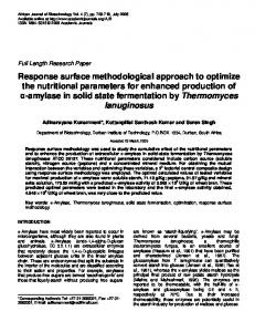
(a)
(b)
Fig. 1. Fig. 1(a) shows the distribution of the data (blue circles) and learned dictionary of size 20 (green) for the data. Note how some atoms are very close to each other, depicted by red circles. Fig. 1(b): learned dictionary of size 9 for the data. Now, the atoms are further spaced apart (best seen in color). Consider data X distributed as in Fig. 1(a). We start with an initial dictionary of size k0 distributed randomly over the unit sphere. We see that, after training, the atoms of the dictionary align themselves according to the data as in Fig. 1(a). After alignment, one can see that some atoms are clumped together in pairs or triplets. When two or more atoms are very close to each other, it is highly unlikely that more than one of them will be used to represent a data point simultaneously due to the sparsity constraint on the representation coefficients. Referring to Fig. 1(a), only one atom per “clump” of atoms will be used per data point for representation.Hence, whenever dictionary atoms get “too close”, we can merge them, leading to a situation more akin to that seen in Fig. 1(b). Since the setting is online, we receive data points in a sequential manner. In the sparse coding step, we have a single data point xt and we obtain the corresponding coefficients αt αt = argmin α
1 kxt − Dαk2 + λkαk1 2
Then, to update the dictionary for known αt0 s, one needs to obtain the solution for � t � 1X 1 Dt = argmin kxi − Dαi k2 + λkαi k1 . t i=1 2 D In the dictionary update stage (refer Algorithm 1), we restrict the atoms to lie on the unit ball unlike [6] so as to make the clustering easier. uj djt = (2) kuj k Note here that we restrict the dictionary atoms to lie on the unit Eucledian ball, and not in it. This makes the clustering easier, by ensuring the vectors are normalized. We do not apply the mean-shift until minIters iterations has passed. This is because, in the online case, we need to wait until the dictionary learning procedure has adapted itself to a sufficient
Inputs : x ∈ Rn ∼ p(x), λ, D0 ∈ Rn×k0 , maxIters, minIters, h Initialize : A ∈ Rk0 ×k0 ← 0, B ∈ Rm×k0 ← D0 , t = 1 ,D0 ← D0 while t ≤ maxIters do Draw xt ∼ p(x) � � αt = argmin 12 kxt − Dt−1 αk2 + λkαk1 α
A ← A + αt αtT B ← B + xt αtT if t ≥ minIters then Dt−1 = M eanShif t(Dt−1 , h) if Dt−1 6= Dt−1 then A ← 0, B ← Dt−1 {resetting past information} h = h/(t − minIters + 1) {for proving convergence, can be omitted} end if end if Compute Dt using Algorithm 2 of [6], with Dt−1 as warm restart t←t+1 end while Output : Dt
amount of data, before we start modifying it. One can think of a degerate case where , after the first iteration, all the dictionary atoms are perfectly aligned, so that all atoms are in the same cluster, leading to a dictionary of size 1 after clustering. To prevent this, we wait for minIters iterations. In most cases, waiting for k0 iterations before running the mean-shift procedure constitutes a sufficient waiting time. After clustering, if the dictionary is shrunk, i.e. Dt 6= Dt , matrices A and B are reset. This is because the “merged” atoms give rise to a new dictionary, and it makes sense to treat the procedure as if restarting the learning algorithm with the new dictionary as an initialization. This can be seen as analogous to periodically flushing the history in the usual online learning scenario. The procedure can be improved by not discarding history corresponding to the atoms in the dictionary that are retained, but a search will require more computations, possibly obliviating the complexity gains acquired by clustering. 3. COHERENCE, COMPLEXITY, CONVERGENCE COLD learns a more incoherent dictionary, achieves speedups in computational complexity and also converges to a local minimum almost surely. Due to space constraints, we defer detailed proofs and analysis exist for a longer version of our work. Fig. 2 pictorially shows how the coherence is reduced as nearby atoms are clustered and replaced by a single atom. For representation purposes, atoms are assumed to lie on the unit circle in two dimensions Smaller dictionaries have lower sample complexity. The amount of reduction in computational complexity depends on the version of mean-shift clustering used. Traditional mean shift has complexity superlinear in the number of data points [4], generally O(k2 ). We consider here this setting and show that even this achieves a reduction in complexity. So by default, faster mean-shift algorithms (e.g. [10]) will perform much better.
Dsize 50 41 100 40 150 50 200 45 ¯ (b) D
(a) D
Fig. 2. Initial dictionary on the unit disc (Fig. 2(a)). The small shaded area corresponds to the angle between the atoms, which decides the initial coherence µ(D). The bumps outside the disc correspond to the modes of the kernel density estimate over the atoms. Fig. 2(b) shows the atoms after clustering, and the corresponding shaded region indicates the angle determining the new coherence. ¯ < µ(D) Clearly µ(D)
It is natural that every mean-shift will not result in a reduction of dictionary size. Suppose M of them do, so that for every mj iterations, j = 0, 1, · · · M ,P the dictionary size reduces sequentially from k0 to kj . Of course, M j=0 mj = n, where n is the number of iterations. Considering the mean-shift itself to have a (maximum) complexity of O(kj2 ), we have the total complexity of COLD to be less than ODL (the method in [6]) provided that we have 2
M X
mj kj2 ≤ nk02
method ODL COLD ODL COLD ODL COLD ODL COLD
time(sec) 11.855 17.748 20.902 18.201 34.913 23.445 49.840 24.148
MSE(std.dev) 0.00474(0.0030) 0.00475(0.0029) 0.00465(0.0030) 0.00471(0.0029) 0.00462(0.0030) 0.00473(0.0029) 0.00461(0.0029) 0.00472(0.0029)
Table 1. Comparison of ODL and COLD on the “background” dataset. The first column indicates the final dictionary size after learning. Note that in case of ODL, final size = initial size. We can see that, as the initial dictionary size increases, COLD is much faster, while the loss in MSE is negligible
this size, and clustering of the atoms will not further reduce the size of the dictionary significantly. In single images, even after a single iteration, the dictionary size reduces and we obtain a significant speedup in the algorithm. For the plot in Fig 3, we used 6000 patches for training, merely to display the speedup of the algorithm. The remainder of the patches constituted the test set. We see that ODL takes 4× in training than COLD. The “jump” observed in the plot is due to the fact that the dictionary size drastically reduces when the mean-shift is applied, and the entire learning process has to be restarted.
(3)
j=0
This inequality will strictly hold as long as mj is large and kj