Using Krylov-Padé Model Order Reduction for Accelerating Design ...

INTERNATIONAL JOURNAL FOR NUMERICAL METHODS IN ENGINEERING Int. J. Numer. Meth. Engng 2010; 00:1–6 Prepared using nmeauth.cls [Version: 2002/09/18 v2.02]

Using Krylov-Pad´e Model Order Reduction for Accelerating Design Optimization of Structures and Vibrations in the Frequency Domain Yao Yue and Karl Meerbergen∗ Departement Computerwetenschappen, Katholieke Universiteit Leuven, Celestijnenlaan 200 A, B-3001 Heverlee, Belgium

SUMMARY In many engineering problems, the behavior of dynamical systems depends on physical parameters. In design optimization, these parameters are determined so that an objective function is minimized. For applications in vibrations and structures, the objective function depends on the frequency response function over a given frequency range and we optimize it in the parameter space. Due to the large size of the system, numerical optimization is expensive. In this paper, we propose the combination of Quasi-Newton type line search optimization methods and Krylov-Pad´e type algebraic model order reduction techniques to speed up numerical optimization of dynamical systems. We prove that Krylov-Pad´e type model order reduction allows for fast evaluation of the objective function and its gradient, thanks to the moment matching property for both the objective function and the derivatives towards the parameters. We show that reduced models for the frequency alone lead to significant speed ups. In addition, we show that reduced models valid for both the frequency range and a line in the parameter space can further reduce c 2010 John Wiley & Sons, Ltd. the optimization time. Copyright key words: (Parameterized) Model Order Reduction, Krylov Methods, Quasi-Newton Optimization, Design Optimization, Structures and Vibrations

1. Introduction Numerical parameter studies of vibration problems arising from applications such as the design of airplane engines, insulation panels along motor ways or in houses, and RCL oscillator circuits are often carried out in order to choose the “optimal” values of the parameters to meet design objectives such as reducing noise, and thus can be viewed as optimization problems. These problems are often computationally extremely expensive, since for each single parameter value, an entire Frequency Response Function (FRF) needs to be computed, which by itself is already quite expensive. The goal of this paper is the efficient solution of design optimization problems arising from structures and vibrations. The objectives of our design optimization problems are to find the values of design parameters so that some norm of the FRF is minimized. When we use the ∞-norm, we have a so-called minimax optimization problem, while with the 2-norm, we minimize some energy norm over a given frequency range. When a sparse linear system solver is directly used for the computation of the FRFs, the gradients are cheaply computed as by-products of the function evaluations. Therefore, Quasi-Newton type methods are good choices for these problems. However, for large scale systems that often occur in real world applications, function evaluations are quite expensive. The computational cost for FRFs has been dramatically reduced by a factor of ten or more by using Model Order Reduction (MOR) techniques [29]. For large scale systems, Krylov-Pad´e type MOR methods are of special interest because their computational costs are relatively low [4]. The goal of MOR is to construct a low order reduced model to approximate the large-scale original model with high accuracy to reduce the computational cost. It has already been successfully applied to many different fields such as

∗ Correspondence

to: Karl Meerbergen, Departement Computerwetenschappen, Katholieke Universiteit Leuven, Celestijnenlaan 200 A, B-3001 Heverlee, Belgium Contract/grant sponsor: Publishing Arts Research Council; contract/grant number: 98–1846389

Received June 3, 2011 c 2010 John Wiley & Sons, Ltd. Copyright

2

YAO YUE AND KARL MEERBERGEN

circuit simulations [13, 33], (vibro) acoustics [29] and MEMS design [18]. Traditionally, we fix all the design parameters and reduce only on the frequency ω to accelerate the evaluations of the corresponding FRF. A similar approach in the structural dynamics community is the Component Mode Synthesis method [26, 34]. Recently, Parameterized MOR (PMOR) [40, 17, 39, 11, 22, 14, 15, 25, 24, 23] was introduced to reduce on both ω and the design parameters. To the knowledge of the authors, the existing attempts to combine MOR/PMOR and optimization focus on efficiently generating a sequence of non-parameterized reduced models, each for one parameter value [34], or building a global reduced model [26, 20]. The flavor of this paper is different: our focus is how to combine MOR/PMOR seamlessly with optimization algorithms, such as how to compute gradients with the reduced model for optimization and how to generate reduced models according to the needs of optimization. If we reduce on all parameters, we can use a single reduced model for the whole parameter space. However, for a system with many design parameters, a reduction on all these parameters is not practical since reducing on more parameters generally results in a drastic increase in the order of the Krylov-Pad´e type reduced model because of the combinatorial explosion in the number of (cross)moments, which increases both the size of the reduced model and the computational cost of building a reduced model. Our approach is to fix most parameters and use PMOR on the parameters or the linear combinations of parameters that are of interest to optimization. If a parameter is allowed to change in the reduced model, we call it a free parameter ; otherwise, we call it a fixed parameter. In this paper, the frequency will always be a free parameter, and in the PMOR case, the other free parameter will be chosen as a linear combination of parameters that corresponds to the line search direction, which is suitable for accelerating line search based optimization algorithms. To efficiently increase the performance of Quasi-Newton type optimization, MOR/PMOR should also be able to approximate gradients. As is well known, Krylov-Pad´e type MOR methods have a moment matching property for the output. More recently, it was proven that the gradient is also matched in the interpolation point [16, 3]. However, for optimization problems, a reduced model should well approximate the gradients in more than just the interpolation point. We will prove that the first order derivatives also satisfy a moment matching property in two-sided MOR/PMOR methods, both for free parameters and for fixed parameters. This means that we can compute gradients accurately via the reduced model for all values of the free parameters in a certain interval. Note that Hessians do not have a moment matching property unless we reduce on all parameters, so Newton-type methods are not favorable. Another advantage of Quasi-Newton methods is that they are effective even when the object function is non-smooth [19, 38], as is the case for ∞norm optimization. To guarantee convergence, we use a backtracking strategy with the Armijo condition [32]. We propose two general frameworks to solve optimal design problems: 1. The MOR Framework : only takes ω as a free parameter. It builds a new reduced model if any design parameter changes; 2. The PMOR Framework : also takes the line search direction as a free parameter. It uses the same reduced model for the computation of all FRFs whose design parameters lie on the search direction in the parameter space. It applies to linear systems that are polynomially dependent on design parameters. If the objective function is non-smooth, particularly when the optimizer is a kink point as is the case in ∞norm optimization, a line search step may contain many backtracking steps to satisfy the Armijo condition so that the Quasi-Newton method can greatly benefit from a PMOR reduced model valid for the search direction. When the objective function is smooth as is the case in 2-norm optimization, the probability that the initial line search point satisfies the Armijo condition is high for Quasi-Newton type optimization methods within the convex region. This implies that backtracking is not often carried out, so that a reduced model in the search direction can seldom be exploited. The paper is organized as follows. In §2, we formulate the optimization problem, present two benchmark problems, and review well established Quasi-Newton optimization methods. Then, we give a brief introduction to MOR and PMOR in §3. We also introduce the two-sided PIMTAP method that will be used for matching moments of the gradients in optimization. Section 4 discusses the moment matching properties for the derivatives, which are not widely known properties of MOR and PMOR methods. In §5, we propose two frameworks to fit MOR and PMOR into the Quasi-Newton type optimization algorithms. In §6, we present the numerical examples for the proposed methods. We conclude the paper in §7. Throughout the paper, we use lower case letters for vectors, upper case letters for matrices, I for identity matrices and 0 for zero matrices. We use ·∗ for the conjugate transpose of a matrix or a vector, and also for −1 the complex conjugate of a complex number. For a nonsingular matrix M , we use M −∗ to denote (M ∗ ) . c 2010 John Wiley & Sons, Ltd. Copyright Prepared using nmeauth.cls

Int. J. Numer. Meth. Engng 2010; 00:1–6

3

ACCELERATING OPTIMIZATION WITH MODEL ORDER REDUCTION

The real part of a complex number z is denoted by 1.

(27)

n o [j] [j] [j] [j] From the relationship (27), we can see that r[1] , r[2] , . . . , r[k] span Kk −G−1 C , r [j] [j] [1] , which can be generated with the standard Arnoldi process. In this way, PIMTAP can generate rectangular moment matching patterns like the one shown in Figure 7(a), where a solid circle at (i, j) means the (i, j)-th moment is matched. Nonrectangular moment matching patterns are sometimes also preferred because in some applications, the high order cross-term moments are not so important. An extreme example is the method proposed in [17] that matches none of the cross-term moments but is still accurate enough for a particular application [17]. For non-rectangular patterns like the one shown in 7(b), PIMTAP uses TAP [23], which can be regarded as an efficient rearrangement of several Arnoldi processes, to generate the Krylov subspaces. We use moment matching vectors to represent a moment matching pattern, where the i-th entry denotes the number of specified moments with an order i w.r.t s. For example, the moment matching pattern shown in Figure 7(b) is represented with (10, 7, 4, 2).

4

λ 6

3 t 2 t 1 t

4 t

t

t

t

t

t

t

t

t

t t

t t

t t

t t

t t

t t

t t

t t

t t

t t t t t t t t t t -s 0 1 2 3 4 5 6 7 8 9 10 (a) The moment matching pattern of PIMTAP via Arnoldi Process. The matched moments spans V(10, 4).

λ 6

3 t 2 t 1 t

t t t

t t

t t

t

t

t

t t t t t t t t t t -s 0 1 2 3 4 5 6 7 8 9 10 (b) An example of moment matching pattern for PIMTAP via TAP.

Figure 7. Illustrations of the moment matching patterns of PIMTAP.

3.5. Two-sided PIMTAP As we will discuss in §4, matching the moments of the gradient require the use of two-sided MOR/PMOR methods if we have fixed parameters. Therefore, we develop a two-sided version of PIMTAP and discuss its moment matching properties to apply PMOR to Quasi-Newton type optimization. Since PIMTAP can be viewed as a rearrangement of several Arnoldi Processes, we can expect that two ∞ X ∞ X
−∗ M sided methods also work for PIMTAP. Expand t = G0 + λG1 + sC0 ` as ζij si λj , where ζij is the i=0 j=0

c 2010 John Wiley & Sons, Ltd. Copyright Prepared using nmeauth.cls

Int. J. Numer. Meth. Engng 2010; 00:1–6

13

ACCELERATING OPTIMIZATION WITH MODEL ORDER REDUCTION

h iT [j] j−1 T 0 1 (i, j)-th moment of t due to (15). Define ζ[i] = (ζi−1 )T , (ζi−1 )T , . . . , (ζi−1 ) . The recursive relationship [j]

[j]

[j]

[j]

[j]

[j]

[j]

−∗ ∗ ∗ of ζ[i] is ζ[i] = −G−∗ [j] C[j] ζ[i−1] . Therefore, ζ[1] , ζ[2] , . . . , ζ[k] span Kk {−G[j] C[j] , ζ[1] }, from whose Krylov

vectors we can obtain the base vectors of the (k, j)-th left Krylov subspace K(l) (k, j). Note that the moment matching patterns of the left Krylov subspace and the right Krylov subspace need not be the same and the only requirement is the number of moments specified by the two patterns to be the same. See Figure 8(a) and Figure 8(b) for an example. Using PIMTAP to obtain V ∈ Cn×k and W ∈ Cn×k , whose column vectors form orthonormal bases for the Krylov subspaces specified by the left and right moment matching patterns respectively, we obtain a two-sided PIMTAP reduced order model
 ˆ 0 + λG ˆ 1 + sCˆ0 x = b, G (28) yˆ = `ˆ∗ x, ˆ 0 = W ∗ G0 V , G ˆ 1 = W ∗ G1 V , Cˆ0 = W ∗ C0 V , ˆb = W ∗ b, `ˆ = V ∗ `. The following theorem shows the where G moment matching properties of our proposed two-sided PIMTAP. ˆ 0 in (28) to be nonsingular, then, the (i − 1, j − 1)-th moment of y in the two-sided Theorem 4. Assume G PIMTAP reduced model and the original model match if any of the following three conditions is satisfied: 1. K(l) (i, j) ⊆ colspan{W } or K(r) (i, j) ⊆ colspan{V }; 2. there exists il , ir ≥ 0, such that K(l) (il , j) ⊆ colspan{W }, K(r) (ir , j) ⊆ colspan{V } and il + ir = i; 3. there exists jl , jr ≥ 0, such that K(l) (i, jl ) ⊆ colspan{W }, K(r) (i, jr ) ⊆ colspan{V } and jl + jr = j. Proof : 1. A direct deduction of the first and the second statements of Theorem 2. 2. A direct deduction of the last statement of Theorem 2. h iT [j] j−1 T 3. Change the roles of λ and ω in PIMTAP. Define rh [i] = (r0j−1 )T , (r1j−1 )T , . . . , (ri−1 ) and we [j]

[j−1]

can find a relationship similar to (27), which we denote as rh [i] = −Gh −1 , for all i > 1. [j] Ch[j] rh [i] This relationship provides an alternative implementation to generate the 2-parameter Krylov subspace. Both of the two implementations generate the same subspace, the subspace spanned by the moments to be matched. Using the result in case 2 for these alternative implementations for K(l) (i, jl ) and K(r) (i, jr ), the (i − 1, j − 1)-th moments of y and yˆ match according to Theorem 2.  Theorem 4 shows that for a linear system with two parameters s and λ, if the left Krylov subspace and the right Krylov subspace use the same rectangular moment matching pattern that specifies k moments, then 3k moments of y and yˆ match. When the moment matching pattern is not rectangular, the number of matched moments is less than 3k. Figure 8 gives an example where the left Krylov subspace and the right Krylov subspace have different moment matching patterns. However, we always use the same moment matching pattern for both Krylov subspaces in this paper because more moments match in this case.

4 3 2 1

λ 6 s s s s s s s s

4 3 2 1

-s

0 1 2 3 4 5 6 7 8 9 10 (a) Moment matching pattern for the left Krylov subspace

λ 6 s s s s s s s s

4 3 2 1

-s

0 1 2 3 4 5 6 7 8 9 10 (b) Moment matching pattern for the right Krylov subspace

λ 6 s s s s s s s s

s s s s s s s s s s s s s s s

-s

0 1 2 3 4 5 6 7 8 9 10 (c) Moment matching pattern for y

Figure 8. Illustrations of the moment matching property of two-sided PIMTAP

c 2010 John Wiley & Sons, Ltd. Copyright Prepared using nmeauth.cls

Int. J. Numer. Meth. Engng 2010; 00:1–6

14

YAO YUE AND KARL MEERBERGEN

4. Derivative Computations via Krylov-Pad´e Type MOR/PMOR As was mentioned in Section 2, MOR/PMOR can only be effective in accelerating parameter optimization problems if also the derivatives are computed via the reduced model. In this section, we discuss the moment matching properties of the derivatives between the original model and the reduced model. We divide this problem into two categories: computation of derivatives w.r.t free variables in the reduced model and computation of derivatives w.r.t fixed variables in the reduced model. We will show that we have moment matching properties for the low order derivatives towards free variables for both one-sided and two-sided MOR/PMOR methods, while we have moment matching properties for the first order derivatives towards fixed variables only for two-sided MOR/PMOR methods. 4.1. Moment Matching Property of Derivatives w.r.t Free Variables Consider system (16), where the output is y = is yˆ =

∞ X

∞ X

mi αi and the corresponding output of the reduced system

i=0

m ˆ i αi . We can derive

i=0 ∞

X dk y = (i + 1)(i + 2) . . . (i + k)mi+k αi , dαk i=0 k

∞

dk yˆ X = (i + 1)(i + 2) . . . (i + k)m ˆ i+k αi . dαk i=0

(29)

k

d y d yˆ Therefore, the i-th moment of dα ˆ i+k k and dαk are (i + 1)(i + 2) . . . (i + k)mi+k and (i + 1)(i + 2) . . . (i + k)m respectively. They match if and only if mi+k = m ˆ i+k , which means the (i + k)-th moments of y and yˆ match. With similar arguments, we can generalize this result to multiparameter cases by the following theorem.

Theorem 5. For the original system (11) and the reduced system (12), the (i1 , i2 , . . . , il )-th moments of ∂ r1 +r2 +···+rl y ∂ r1 +r2 +···+rl yˆ and match if and only if the (i1 + r1 , i2 + r2 , . . . , il + rl )-th moments of y ∂pr11 ∂pr22 · · · ∂prl l ∂pr11 ∂pr22 · · · ∂prl l and yˆ match. Now we illustrate Theorem 5 with the linear system (25) parameterized with s and λ. If the moment matching pattern of y and yˆ is given by Figure 9(a), we can obtain the moment matching pattern of ∂y ∂s by shifting Figure 9(a) one step leftward as is shown in Figure 9(b); similarly, we can obtain the moment ∂y matching pattern of ∂λ by shifting Figure 9(a) one step downward as is shown in Figure 9(c). 4 3 2 1

λ 6 s s s s s s s s s s s s s s s s s s s s s s s -s

0 1 2 3 4 5 6 7 8 9 10 (a) Moment matching pattern for y

4 3 2 1

λ 6 s s s s s s s s s s s s s s s s s s s

4 3 2 1

-s

0 1 2 3 4 5 6 7 8 9 10 (b) Moment matching pattern for ∂y ∂s

λ 6 s s s s s s s s s s s s s

-s

0 1 2 3 4 5 6 7 8 9 10 ∂y (c) Moment matching pattern for ∂λ

Figure 9. Illustrations of the Derivative Computation of a System Containing Two Parameters.

4.2. Moment Matching Properties of the First Order Derivatives w.r.t. Fixed Variables in the Reduced Model Assume that we also have a fixed parameter q, which is free to change in the original model but is fixed to q0 in the reduced model:  L(p1 , p2 , . . . , pl |q)x = b, (30) y = `∗ x. The first order derivative w.r.t q can be computed as ∂y ∗ −1 ∂L(p1 , p2 , . . . , pl |q) = −` L(p , p , . . . , p |q = q ) L(p1 , p2 , . . . , pl |q = q0 )−1 b. (31) 1 2 l 0 ∂q q=q0 ∂q q=q0 ∂ yˆ To see the moment matching properties between ∂y and , we prove the following more general ∂q ∂q q=q0

q=q0

theorem. c 2010 John Wiley & Sons, Ltd. Copyright Prepared using nmeauth.cls

Int. J. Numer. Meth. Engng 2010; 00:1–6

15

ACCELERATING OPTIMIZATION WITH MODEL ORDER REDUCTION

Theorem 6. Consider the system pair (11) and (12) and assume that K(r) (i1 + 1, i2 + 1, . . . , il + 1) ⊆ colspan{V },

K(r) (i1 + 1, i2 + 1, . . . , il + 1) ⊆ colspan{V }

(32)

and all conditions for Proposition 1 are true. ˆ 1 , p2 , . . . , pl ) Let B(p1 , p2 , . . . , pl ) : Cp → Cn×n be a matrix function and define B(p ∗ W B(p1 , p2 , . . . , pl )V . Then, it follows that the (i1 , i2 , . . . , il )-th moment of `∗ L(p1 , p2 , . . . , pl )−1 B(p1 , p2 , . . . , pl )L(p1 , p2 , . . . , pl )−1 b,

= (33)

denoted by mB (i1 , i2 , . . . , il ), matches the (i1 , i2 , . . . , il )-th moment of ˆ 1 , p2 , . . . , pl )−1 B(p ˆ 1 , p2 , . . . , pl )L(p ˆ 1 , p2 , . . . , pl )−1ˆb, `ˆ∗ L(p

(34)

denoted by m ˆ B (i1 , i2 , . . . , il ). Proof : We only give a proof for the one-parameter case to clarify the idea. Assume that B(p1 ) =

∞ X

Bj pj1 . By

j=0 ∞ X

the definitions (14) and (15), we have `∗ L(p1 )−1 =

ζ ∗ (j)pj1 ,

L(p1 )−1 b =

j=0

 ∗

−1

` L(p1 )

−1

B(p1 )L(p1 )

b=

∞ X

ζ

(j)pj1 

j=0

r(j)pj1 . Therefore,

j=0

 ∗

∞ X

∞ X

! Bk pk1

∞ X

! r(m)pm 1

(35)

m=0

k=0

and X

mB (i1 ) =

ζ ∗ (j)Bk r(m)

(36)

j+k+m=i1

Similarly, ˆ 1 )−1 B(p ˆ 1 )L(p ˆ 1 )−1ˆb = `∗ L(p ˆ 1 )−1 W ∗ B(p1 )V L(p ˆ 1 )−1ˆb `∗ L(p  ∗ ! ∞ ∞ X X j k ( = Bk p1 W ζˆ j)p1  j=0

and m ˆ B (i1 ) =

X

! V

rˆ(m)pm 1

(37)

m=0

k=0



∞ X

∗   ˆ Bk V rˆ(m) W ζ(j)

(38)

j+k+m=i1

ˆ = ζ(j) and V rˆ(j) = r(j) for all 0 ≤ j ≤ i, According to Proposition 1 and the assumption (32), W ζ(j) and comparing the right hand sides of (36) and (38) leads to mB (i1 ) = m ˆ B (i1 ).  The moment matching properties for derivatives are direct results of Theorem 6 because the right hand side of (31) is independent of q and thus, it is only a special case of (33). Although Theorem 6 holds for all parameters, Theorem 5 gives more precise results for free parameters. For example, for the k-order reduced system (24), we know from Theorem 2 and Theorem 5 that the first 2k − 1 moments of the first order derivative match, but Theorem 6 can only tell us that the first k moments match. 4.3. Conclusions and Hints for Optimization Consider the system (11). Suppose that we reduce on p1 , p2 , . . . , pt (t ≤ l) and fix the remaining parameters. We define span{p1 , p2 , . . . , pt } as the reduced parameter space. We consider the following options in an optimization scenario. • If we reduce on all parameters, both gradient and Hessian will have moment matching properties, which means that the reduced model can be used to accelerate both Newton or Quasi-Newton optimization algorithms. However, this approach is undesirable for systems with many parameters, since the cost for building such a model would be very high. c 2010 John Wiley & Sons, Ltd. Copyright Prepared using nmeauth.cls

Int. J. Numer. Meth. Engng 2010; 00:1–6

16

YAO YUE AND KARL MEERBERGEN

• If we have fixed parameters, we have to use two-sided MOR/PMOR methods rather than one-sided methods to achieve a moment matching property for the gradient. More specifically, for each fixed ∂y on the whole reduced parameter γi (i = t + 1, t + 2, . . . , l), we have a moment matching property for ∂γ i parameter space. However, the Hessian does not have moment matching properties for both one-sided and two-sided cases. We have observed in numerical tests that the Hessian is not well approximated in general; even its positive definiteness is not preserved in some test cases. Therefore, the reduced model can be used for Quasi-Newton methods, but not for Newton methods. This explains why we chose two-sided MOR/PMOR for the model reduction part and chose Quasi-Newton type method for the optimization part.

5. Two Frameworks to Use MOR/PMOR in Accelerating Optimization As was analyzed in §2, parameter optimization of large scale linear systems is computationally expensive. It requires a large number of function and derivative evaluations of a large-scale system. Our idea is to use two-sided Krylov-Pad´e type MOR/PMOR to reduce the computational cost since it can accurately compute both the function values and gradients thanks to the moment matching properties. In this section, we propose two frameworks that apply Krylov-Pad´e type MOR/PMOR to Quasi-Newton type optimization algorithms. Both these frameworks use MOR/PMOR for efficient numerical computations, while taking advantage of Quasi-Newton type methods to have super-linear convergence rate. 5.1. The MOR Framework: One Reduced Model for Each Inner Phase In this part, we develop the MOR Framework for efficiently computing an entire Inner Phase by a reduced model with all design parameters fixed. Remind from §2.3.5 that the Inner Phase carries out numerical integration or one-dimensional optimization in the frequency domain and is quite computationally expensive for large-scale problems. The motivation of the MOR Framework is that since all design parameters are fixed for an Inner Phase, we can first use SOAR to reduce on ω and then use the SOAR reduced model ∂y can be computed accurately near the for all computations in that Inner Phase. Thanks to Theorem 6, ∂γ i interpolation point. In the MOR Framework, we need only one LU factorization for MOR at (ω0 , γ (0) ), where ω0 denotes the frequency shift and γ (0) denotes the fixed design parameter value, rather than at (ω, γ (0) ) for all relevant ω’s in the Inner Phase. Therefore, the acceleration by the MOR Framework depends on how much can the system dimension be reduced and how many ω values are used by the Inner Phase. In many applications in mechanics and acoustics, the acceleration by the MOR Framework should be efficient since 1.) a very low order reduced model compared with the order of the original model is able to capture the dominant behavior of the FRF; 2.) both numerical integration and one-dimensional Quasi-Newton optimization need LU factorizations at various ω values. 5.2. The PMOR Framework: One Reduced Model for Each Line Search Iteration in the Outer Phase Since PIMTAP can reduce on more than one variable, we expect it to accelerate design optimization more efficiently. For the acoustic box optimization problem, we can reduce on both iωγ and −ω 2 with G0 = K, G1 = C, C0 = M , λ = iωγ and s = −ω 2 and use the reduced model for the whole optimization. In general, however, we may have several parameters (say γ1 , γ2 , . . . , γk ) and it is impractical to reduce on all of them. Using the PIMTAP prototype (25), we can reduce on one more parameter other than the frequency. So an interesting topic is how to choose the design parameter that we want to reduce on. A straightforward round-robin approach is to reduce on the [1 + (i − 1) mod k]-th parameter at the i-th iteration. However, this scheme will result in a slow convergence rate in optimization because of the zigzag path used. Instead, the PMOR Framework will use PIMTAP to reduce on ω and an additional parameter α that is used to define points on the search line. We now discuss the working procedure of the PMOR Framework in more detail. Suppose at the j-th iteration, we have the iterate γ (j) and the search direction d(j) . We first generate the j-th PIMTAP reduced model by taking the interpolation point as γ (j) and reducing on both the frequency ω and the line search direction d(j) . So system (5) is reformulated for γ = γ (j) + αd(j) as
 K(γ (j) + αd(j) ) + iωC(γ (j) + αd(j) ) − ω 2 M (γ (j) + αd(j) ) x(ω, γ (j) + αd(j) ) = f, (39) y(ω, γ) = `∗ x(ω, γ (j) + αd(j) ). c 2010 John Wiley & Sons, Ltd. Copyright Prepared using nmeauth.cls

Int. J. Numer. Meth. Engng 2010; 00:1–6

ACCELERATING OPTIMIZATION WITH MODEL ORDER REDUCTION

When K(γ), C(γ) and M (γ) are all matrix polynomials of γ, we can linearize the system (39) as  (  ˜ + αC˜ + iω M ˜ x K ˜ = f˜, ∗ ˜ y=` x ˜,

17

(40)

˜ similar to what we have done in (21). For the linearization (40), we can use two-sided with a nonsingular K ˜ λ = α and s = iω and ˜ G1 = C, ˜ C0 = M ˜ , b = f˜, ` = `, PIMTAP to reduce on α and iω with G0 = K, obtain a reduced model that can approximate g and ∇g on the search direction with moment matching properties according to Proposition 1 and Theorem 6. Therefore, all backtracking steps in the Armijo search can be efficiently conducted. Assume that after the j-th line search, we accept γ (j+1) as the next iterate. Since we can use the j-th reduced model to compute both the function value and the gradient accurately, the Quasi-Newton search direction d(j+1) can also be determined with the j-th reduced model. Then we can build the (j + 1)-st reduced model with γ (j+1) and d(j+1) . 5.3. Remarks on the MOR Framework and the PMOR Framework 1. In both frameworks, the optimization follows the same path as a direct method that deals directly with the unreduced original model if all reduced models are accurate enough, which is often the case in practice since a reduced model with a much smaller size than the original model is sufficiently accurate for optimization for many applications. 2. For ∞-norm optimization, the PMOR Framework is often more effective since backtracking often occurs for the non-smooth objective function in ∞-norm optimization and the PMOR Framework makes the backtracking steps very efficient; 3. For 2-norm optimization, the MOR Framework is often more effective because 1.) after the first few iterations, the initial points in line searches predicted by Quasi-Newton algorithms almost always satisfy the Armijo condition for the convex objective function in 2-norm optimization, so few backtracking occurs and a PMOR reduced model is only used for one point on the search line; 2.) the size of a PMOR reduced model typically needs to be larger than the size of a MOR reduced model to achieve similar accuracy for evaluations at points other than the PMOR interpolation point; 4. The convergence of the PMOR Framework mainly depends on the approximation accuracy at the interpolation points. When the optimization algorithms converges, the step length α approaches zero, which suggests 1.) higher order moments w.r.t α become less important; 2.) if a reduced model is accurate enough for γ (k) , it should also be somehow accurate for γ (k+1) . This remark may help the selection of the moment matching patterns for two-sided PIMTAP in the PMOR Framework. We should choose more moments for ω and less for both α and the cross-moments of ω and α. In this way, we exploit the flexibility of the non-rectangular moment patters provided by PIMTAP to obtain smaller reduced models. 5. The MOR Framework is more general than the PMOR Framework. When any of K(γ), C(γ) or M (γ) is not a lower-order matrix polynomial, or even cannot be easily approximated by a lower-order matrix polynomial, the PMOR Framework cannot work efficiently or even fails to work, but the MOR Framework can easily be applied with no change.

6. Numerical Results and Analysis In this section, we apply the MOR Framework and the PMOR Framework developed in §5 to the two design optimization problems described in §2. All our codes are implemented with the C++ package GLAS [27], through whose bindings [31] we solve large-scale sparse linear equations with MUMPS [1] and small scale dense linear equations with LAPACK [2]. All numerical tests are run using a DELL Latitude E6400 with TM R Intel Core 2 Duo 2.66GHz CPU and 4GB of main memory. 6.1. Acoustic Box Design Problem For the acoustic box design problem, we implemented both the MOR Framework and the PMOR Framework for ∞-norm optimization and 2-norm optimization. We also used the direct solver for the original nonreduced model for all computations as a reference to show the effectiveness of the two frameworks. Table II c 2010 John Wiley & Sons, Ltd. Copyright Prepared using nmeauth.cls

Int. J. Numer. Meth. Engng 2010; 00:1–6

18

YAO YUE AND KARL MEERBERGEN

and Table IV indicate that MOR/PMOR is effective even when applied to a relatively small scale system with 1131 DOFs. Table III and Table V show the numerical results when the finite difference model has 19683 DOFs. In both examples, the grid search step length, the frequency range and the backtracking factor are set to 4 Hz, [1 Hz, 11 Hz] and 0.5 respectively. The initial value is γ = 0.3 and we use 100 interpolation points for numerical integrations. For all MOR/PMOR processes, we shift the interpolation point to 6 Hz before conducting the reduction. In all test cases, the PMOR Framework is cheaper but locates the optimizer more accurately. This implies that the PMOR Framework outperforms the MOR Framework when the system has only one design parameter since only one reduced model is needed for the whole optimization. 6.2. Floor Damper Design Problem In this section, we apply the MOR Framework and the PMOR Framework for both ∞-norm optimization and 2-norm optimization of the floor damper design problem. We used two different finite element models for the floor damper: a model with 280 DOFs obtained from a 10 × 10 uniform mesh and a model with 29800 DOFs obtained from a 100×100 uniform mesh. The feasible region is [ 1 N/m, 1010 N/m ]×[ 1 Ns/m, 1010 Ns/m ] and (0) (0) the initial point is γ (0) = [ k1 , c1 ] =[ 107 N/m, 107 Ns/m ]. For parameter values lying outside the feasible region, we assign their function values to be the constant g(γ (0) ), which is an upper bound for the optimizer. Because we use the Armijo condition for line searches, the optimization algorithm can never accept points lying outside the feasible region.   Kf 0 For the floor damper model (9), K0 = is singular, so we first shift the interpolation point to 0 0   ωL +ωH 2

to make MOR/PMOR applicable. In the j-th iteration, given the current iterate   (j) (j) and the search direction d1 , d2 , the system (9) can be rewritten as ω0 =

  K11    0   

0 I



(j)

 +α

C11 0

C12 0

(j)



 + i(ω − ω0 )

(j)

M11 −I

M12 0

(j)

   x f = , i(ω − ω0 )x 0   x y = [`∗ , 0T ] . i(ω − ω0 )x

(j)

(j)

k1 , c1

 

(j)

(41)

(j)

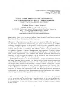
where K11 = K0 +k1 K1 +iω0 c1 K1 −ω02 M , C11 = d1 K1 +iω0 d2 K1 , C12 = d2 K1 , M11 = c1 K1 +2iω0 M and M12 = M . First, we consider ∞-norm optimization for the floor damper design problem. For the optimization of both the 280-order model and the 29800-order model, the frequency range is [2 Hz, 200 Hz] and the grid search interval is 4 Hz respectively. The backtracking factor is set to 0.5 and the proportional damping ratio cp = 0.02. Table VI shows that both the MOR Framework and the PMOR Framework work well in reducing the optimization time. For a relatively large problem shown in Table VII, the direct method would need more than eleven hours to run, while for the MOR Framework and the PMOR Framework, we need only less than an hour to finish the optimization, which is good news for actual designs in industry. From Table VI and Table VII, we can see that ∞-norm optimization involves many backtracking steps, which makes the PMOR Framework more efficient than the MOR Framework. Now we turn to the 2-norm optimization problem. The problem setting is the same as what we used for ∞-norm optimization except that we used 100 uniform grid points to carry out numerical integrations based on the Trapezoidal rule. The numerical results in Table VIII and Table IX show that for 2-norm optimization, the MOR Framework is more efficient than the PMOR Framework since backtracking is not often required. This coincides with our discussion in §5.3. The results in Table VI and Table VIII indicate that 2-norm optimization is more efficient than ∞-norm optimization. On the one hand, the optimization of the 2-norm converges faster because its objective function is smoother. To show this, we plotted kγk − γk−1 k for the example of Table VI and the example of Table VIII in Figure 10. On the other hand, backtracking does not occur frequently for Armijo line searches in 2 norm optimization as the objective function is convex and smooth; while for ∞-norm optimization, the optimizer is often a kink point. Around the kink optimizer, a Quasi-Newton type method may generate a too large initial step length, in which case it needs many backtracking steps to satisfy the Armijo condition. So, the last steps of the ∞-norm optimization become more expensive. This problem can easily be alleviated by using the c 2010 John Wiley & Sons, Ltd. Copyright Prepared using nmeauth.cls

Int. J. Numer. Meth. Engng 2010; 00:1–6

ACCELERATING OPTIMIZATION WITH MODEL ORDER REDUCTION

19

PMOR Framework since in that case, all backtracking steps use the same reduced model. Our experience also shows that if 2-norm optimization starts from a point in the non-convex region, the number of backtracking steps increases, which may make the PMOR Framework with Armijo line searches also outperform the MOR Framework. 107

2-norm ∞-norm

106

|γk − γk−1 |

105 104 103 102 101 100 10−1 0

2

4

6

8

10

12

14

16

18

Iteraion k

Figure 10. Comparison of Convergence Rate for 2-norm and ∞-norm Optimization

In our numerical results, we tried to find the smallest reduced model size that achieves acceptable approximation accuracy so that the performance of the two frameworks are comparable. These approximation errors lead to some differences in the converging process, such as the number of iterations required to converge. Actually, if we increase these sizes a little bit, the reduced models become much more accurate and these differences become even smaller.

6.3. MOR Eases the Choice of Optimization Parameters For both 2-norm optimization and ∞-norm optimization, we have a trade-off between the optimization performance and the computational cost in the Inner Phase. In the 2-norm case, we need to use many interpolation points to guarantee the accuracy of the numerical integration, which is computationally expensive when the order of the problem is high. For ∞-norm optimization, the step length of the grid search should be fine enough to avoid missing the global optimizer. How to choose the number of interpolation points or grid points is by itself a complicated optimization problem. But if we use MOR/PMOR, all evaluations in an Inner Phase are computed with the same reduced model and even if we use a fine grid to increase accuracy, the computational cost does not significantly increase compared with a direct method. In our numerical examples, we used relatively few grid points to make a fair comparison between the direct method and MOR/PMOR methods.

6.4. Open problem: Determination of the Size of the Reduced Model An open problem is how large the dimensions of subspaces should be for practical use in numerical optimization. In this paper, we have shown that accurate results can be approximated well with the results obtained from MOR/PMOR. In practice, however, the number of vectors should be determined by an error estimator. One possibility is to use error estimations as in [9], or use the residual norm for the systems (K(γ) + iωC(γ) − ω 2 M (γ))x = 2

∗

(K(γ) + iωC(γ) − ω M (γ)) t =

f `

The computed solutions are then the exact solution of a perturbed system. Such residual norms are cheaply computed. See, e.g., [36, 29, 30]. The development of practical heuristics is future work. c 2010 John Wiley & Sons, Ltd. Copyright Prepared using nmeauth.cls

Int. J. Numer. Meth. Engng 2010; 00:1–6

20

YAO YUE AND KARL MEERBERGEN

7. Conclusion In this paper, we presented a Quasi-Newton type line search optimization method for the solution of optimization problems arising from design optimization of vibrations and structures. We used MOR/PMOR in order to reduce the computational cost. We hereby compare MOR reduced models for the frequency response function with fixed parameters, and PMOR reduced models for the frequency and the search direction. When the objective function is the ∞-norm of the frequency response function, the better choice is using PMOR reduced models valid for the searched direction; while when the objective function is the 2-norm of the frequency response function, the best choice is using MOR reduced models.

ACKNOWLEDGEMENTS

This paper presents research results of the Belgian Network DYSCO (Dynamical Systems, Control, and Optimization), funded by the Interuniversity Attraction Poles Programme, initiated by the Belgian State Science Policy Office. The research is also partially funded by the Research Council K.U.Leuven grants CoE EF/05/006 (Optimization in Engineering) and OT/10/038 (Multi-parameter model order reduction and its applications). The scientific responsibility rests with its authors.

REFERENCES 1. P. R. Amestoy, I. S. Duff, J. Koster, and J.-Y. L’Excellent. A fully asynchronous multifrontal solver using distributed dynamic scheduling. SIAM Journal of Matrix Analysis and Applications, 23:15–41, 2001, doi:10.1.1.34.5808. 2. E. Anderson, Z. Bai, C. Bischof, S. Blackford, J. Demmel, J. Dongarra, J. Du Croz, A. Greenbaum, S. Hammarling, A. McKenney, and D. Sorensen. LAPACK Users’ Guide. Society for Industrial and Applied Mathematics, Philadelphia, PA, third edition, 1999. 3. A. Antoulas, C. Beattie, and S. Gugercin. Interpolatory model reduction of large-scale dynamical systems. In Efficient Modeling and Control of Large-Scale Systems. Springer-Verlag, 2010. 4. A. C. Antoulas and D. C. Sorensen. Approximation of large-scale dynamical systems: an overview. International Journal of Applied Mathematics and Computer Science, 11(5):1093–1121, 2001. 5. W. E. Arnoldi. The principle of minimized iterations in the solution of the matrix eigenvalue problem. Quarterly of Applied Mathematics, 9(17):17–29, 1951. 6. Z. Bai, K. Meerbergen, and Y. Su. Arnoldi methods for structure-preserving dimension reduction of second-order dynamical systems. In Dimension reduction of large-scale systems, pages 173–189. Springer, 2005. 7. Z. Bai and Y. Su. Dimension reduction of large-scale second-order dynamical systems via a second-order Arnoldi method. SIAM Journal on Scientific Computing, 26(5):1692–1709, 2005, doi:10.1137/040605552. 8. Z. Bai and Y. Su. SOAR: a second-order Arnoldi method for the solution of the quadratic eigenvalue problem. SIAM Journal on Matrix Analysis and Applications, 26(3):640–659, 2005, doi:10.1137/S0895479803438523. 9. Z. Bai and Q. Ye. Error estimation of the Pad´ e approximation of transfer functions via the Lanczos process. ETNA, 7:1–17, 1998. 10. C. R. Calladine. Theory of Shell Structures. Cambridge University Press, 1989. 11. L. Daniel, O. C. Siong, L. S. Chay, K. H. Lee, and J. White. A multiparameter moment-matching model-reduction approach for generating geometrically parameterized interconnect performance models. Computer-Aided Design of Integrated Circuits and Systems, IEEE Transactions on, 23(5):678–693, 2004, doi:10.1109/TCAD.2004.826583. 12. P. J. Davis and P. Rabinowitz. Methods of Numerical Integration. Dover Publications, 2nd edition, 2007. 13. P. Feldman and R. W. Freund. Efficient linear circuit analysis by Pad´ e approximation via the Lanczos process. IEEE Trans. Computer-Aided Design, 14(5):639–649, 1995, doi:10.1109/43.384428. 14. L. Feng. Parameter independent model order reduction. Mathematics and Computers in Simulation, 68:221–234, 2005, doi:10.1088/0960-1317/20/4/045030. 15. L. H. Feng, E. B. Rudnyi, and J. G. Korvink. Preserving the film coefficient as a parameter in the compact thermal model for fast electrothermal simulation. IEEE Trans. Computer-Aided Design, 24(12):1838–1847, 2005, doi:10.1109/TCAD.2005.861422. 16. S. Gugercin, A. C. Antoulas, and C. Beattie. H2 model reduction for large-scale linear dynamical systems. SIAM journal on matrix analysis and applications, 30(2):609–638, 2008, doi:10.1137/060666123. 17. P. Gunupudi and M. Nakhla. Multi-dimensional model reduction of VLSI interconnects. In Custom Integrated Circuits Conference, 2000. Proceedings of the IEEE 2000, pages 499–502, 2000. 18. J. S. Han, E. B. Rudnyi, and J. G. Korvink. Efficient optimization of transient dynamic problems in MEMS devices using model order reduction. Journal of Micromechanics and Microengineering, 15(4):822–832, 2005, doi:10.1088/09601317/15/4/021. 19. C. Lemar´ echal. Numerical experiments in nonsmooth optimization. In E. Nurminski, editor, Progress in Nondifferentiable Optimization, pages 61–84, 1982. 20. A. T.-M. Leung and R. Khazaka. Parametric model order reduction technique for design optimization. In ISCAS 2005. IEEE International Symposium on, pages 1290–1293 Vol.2. IEEE, 2005. 21. A. S. LEWIS and M. L. OVERTON. Nonsmooth optimization via BFGS. Technical report, New York University, 2008. 22. X. Li, P. Li, and L. T. Pileggi. Parameterized interconnect order reduction with explicit-and-implicit multi-parameter moment matching for inter/intra-die variations. In Proceedings of the 2005 IEEE/ACM International conference on Computer-aided design, pages 806–812. IEEE Computer Society Washington, DC, USA, 2005. 23. Y.-T. Li, Z. Bai, and Y. Su. A two-directional Arnoldi process and its application to parametric model order reduction. Journal of Computational and Applied Mathematics, 226(1):10–21, 2009, doi:10.1016/j.cam.2008.05.059. c 2010 John Wiley & Sons, Ltd. Copyright Prepared using nmeauth.cls

Int. J. Numer. Meth. Engng 2010; 00:1–6

ACCELERATING OPTIMIZATION WITH MODEL ORDER REDUCTION

21

24. Y.-T. Li, Z. Bai, Y. Su, and X. Zeng. Parameterized model order reduction via a two-directional Arnoldi process. In Proceedings of the 2007 IEEE/ACM international conference on Computer-aided design, pages 868–873, 2007. 25. Y.-T. Li, Z. Bai, Y. Su, and X. Zeng. Model order reduction of parameterized interconnect networks via a Two-Directional Arnoldi process. Computer-Aided Design of Integrated Circuits and Systems, IEEE Transactions on, 27(9):1571–1582, 2008, doi:10.1109/TCAD.2008.927768. 26. G. Masson, B. A. Brik, S. Cogan, and N. Bouhaddi. Component mode synthesis (CMS) based on an enriched ritz approach for efficient structural optimization. Journal of Sound and Vibration, 296(4-5):845–860, 2006, doi:10.1016/j.jsv.2006.03.024. 27. K. Meerbergen. Glas (Generic Linear Algebra Software). http://people.cs.kuleuven.be/~karl.meerbergen/glas/. 28. K. Meerbergen. The solution of parametrized symmetric linear systems. SIAM journal on matrix analysis and applications, 24(4):1038–1059, 2003, doi:10.1137/S0895479800380386. 29. K. Meerbergen. Fast frequency response computation for Rayleigh damping. International Journal for Numerical Methods in Engineering, 73(1):96–106, 2008, doi:10.1002/nme.2058. 30. K. Meerbergen and Z. Bai. The Lanczos method for parameterized symmetric linear systems with multiple right-hand sides. SIAM Journal on Matrix Analysis and Applications, 31(4):1642–1662, 2010, doi:10.1137/08073144X. 31. K. Meerbergen, K. Fresl, and T. Knapen. C++ bindings to external software libraries with examples from BLAS, LAPACK, UMFPACK, and MUMPS. ACM Transactions on Mathematical Software, 36(4), 2009. 32. J. Nocedal and S. Wright. Numerical Optimization. Springer, 2nd edition, 2006. 33. A. Odabasioglu, M. Celik, and L. T. Pileggi. PRIMA: passive reduced-order interconnect macromodeling algorithm. In ICCAD ’97: Proceedings of the 1997 IEEE/ACM international conference on Computer-aided design, pages 58–65, Washington, DC, USA, 1997. IEEE Computer Society. 34. D. A. Perdahcıo˘ glu, M. H. M. Ellenbroek, H. J. M. Geijselaers, and A. de Boer. Updating the CraigBampton reduction basis for efficient structural reanalysis. International Journal for Numerical Methods in Engineering, 85(5):607–624, 2011, doi:10.1002/nme.2983. 35. B. Salimbahrami and B. Lohmann. Order reduction of large scale second-order systems using Krylov subspace methods. Linear Algebra and its Applications, 415(2-3):385–405, 2006, doi:10.1016/j.laa.2004.12.013. 36. V. Simoncini and F. Perotti. On the numerical solution of (λ2 A + λB + C)x = b and application to structural dynamics. SIAM Journal on Scientific Computing, 23(6):1875–1897, 2002, doi:10.1137/S1064827501383373. 37. T. Z. U. J. SU and R. CRAIG. Model reduction and control of flexible structures using Krylov vectors. Journal of guidance, control, and dynamics, 14(2):260–267, 1991, doi:10.2514/3.20636. 38. J. Vlˇ ek and Lukˇsan. Globally convergent variable metric method for nonconvex nondifferentiable unconstrained minimization. Journal of Optimization Theory and Applications, 111(2):407–430, 2001, doi:10.1023/A:1011990503369. 39. D. S. Weile, E. Michielssen, and K. Gallivan. Reduced-order modeling of multiscreen frequency-selective surfaces using Krylov-based rational interpolation. IEEE transactions on antennas and propagation, 49(5):801–813, 2001, doi:10.1109/8.929635. 40. D. S. Weile, E. Michielssen, and E. Grimme. A method for generating rational interpolant reduced order models of twoparameter linear systems. Applied Mathematics Letters, 12(5):93–102, 1999, doi:10.1016/S0893-9659(99)00063-4.

Tables

Table II. Numerical Results of ∞-norm optimization for a Small-scale Acoustic Box Problem Matrix Size Computed Optimizer γ Objective at Optimizer Relative Error of Optimizer Relative Error of Objective CPU Time

Direct Method

The MOR Framework

The PMOR Framework

1131 0.5431165101 0.07357485572 0 0 5.26s

21 0.5431165094 0.07357485572 1.322508937e-09 1.697592052e-15 3.24s

(12, 9, 6, 3)k 0.5431165102 0.07357485572 2.446927891e-10 9.431066954e-16 0.99s

Table III. Numerical Results of ∞-optimization for a Large-scale Acoustic Box Problem Direct Method The MOR Framework The PMOR Framework Matrix Size 19683 Computed Optimizer γ 0.5510131227 Objective at Optimizer 0.06061629893 Relative Error of Optimizer 0 Relative Error of Objective 0 CPU Time 279.38s

k For

21 0.5510131276 0.06061629893 8.914752842e-09 1.4194579e-14 83.91s

(12, 9, 6, 3) 0.5510131227 0.06061629893 1.090450801e-11 5.094022304e-14 34.88s

the PMOR Framework, we show the moment matching vector of two-sided PIMTAP instead to be more specific.

c 2010 John Wiley & Sons, Ltd. Copyright Prepared using nmeauth.cls

Int. J. Numer. Meth. Engng 2010; 00:1–6

22

YAO YUE AND KARL MEERBERGEN

Table IV. Numerical Results of 2-norm optimization for a Small-scale Acoustic Box Problem Matrix Size Computed Optimizer γ Objective at Optimizer Relative Error of Optimizer Relative Error of Objective CPU Time

Direct Method

The MOR Framework

The PMOR Framework

1131 0.4211509312 0.1335686059 0 0 21.78s

25 0.4211676558 0.133568606 3.971165732e-05 7.455717495e-10 2.54s

(12, 9, 6, 3) 0.4211498197 0.1335686059 2.639178282e-06 2.822549364e-12 1.1s

Table V. Numerical Results of 2-norm optimization for a Large-scale Acoustic Box Problem Matrix Size Computed Optimizer γ Objective at Optimizer Relative Error of Optimizer Relative Error of Objective CPU Time

Direct Method

The MOR Framework

The PMOR Framework

19683 0.4094729565 0.1161370131 0 0 1887.06s

21 0.4094891639 0.1161370132 3.958132505e-05 7.9512616e-10 72.9s

(12, 9, 6, 3) 0.4094696543 0.1161370131 8.064358032e-06 3.282526569e-11 28.92s

Table VI. Numerical Results of ∞-norm Optimization for a Small-scale Floor Damper Problem Matrix Size Computed Optimizer (k1 , c1 ) Optimized Objective Number of Iterations Total Backtracking Steps∗∗ Relative Error of Optimizer Relative Error of Objective CPU Time

Direct Method

The MOR Framework

The PMOR Framework

280 (11500243, 109352.8125) 2317774917 18 152 0 0 118.69s

7 (11500242.91, 109352.8112) 2317774964 18 152 7.960963132e-09 2.022068017e-08 5.07s

(7, 3) (11500242.74, 109352.8405) 2317774827 16 111 2.34067375e-08 3.912525703e-08 1.14s

Table VII. Numerical Results of ∞-norm Optimization for a Large-scale Floor Damper Problem Direct Method

The MOR Framework

The PMOR Framework

Matrix Size 29800 7 (7, 3) Computed Optimizer (k1 , c1 ) (11677301.94, 115621.0844) (11677156.58, 15632.289) (11677316, 115620.0156) Optimized Objective 237859351.5 237857438.1 237859525.1 Number of Iterations 15 15 14 Total Backtracking Steps 108 120 90 Relative Error of Optimizer 0 1.24849323e-05 1.207336986e-06 Relative Error of Objective 0 8.039805108e-06 7.37015408e-07 CPU Time 41069s 1104s 417s

∗∗ This

number does not count null backtracking steps, which lie out of the feasible region and are immediately discarded without any computation. c 2010 John Wiley & Sons, Ltd. Copyright Prepared using nmeauth.cls

Int. J. Numer. Meth. Engng 2010; 00:1–6

ACCELERATING OPTIMIZATION WITH MODEL ORDER REDUCTION

23

Table VIII. Numerical Results of 2-norm Optimization for a Small-scale Floor Damper Problem Matrix Size Computed Optimizer (k1 , c1 ) Optimized Objective Number of Iterations Total Backtracking Steps Relative Error of Optimizer Relative Error of Objective CPU Time

Direct Method

The MOR Framework

The PMOR Framework

280 (11773499.86, 95303.15231) 1.4681996e+11 12 3 0 0 17.05s

7 (11773499.86, 95303.15231) 1.468199567e+11 12 3 2.284557138e-13 4.157143049e-15 0.52s

(7, 3) (11773499.75, 95303.15197) 1.468199567e+11 12 3 9.460980157e-09 9.561429013e-15 0.82s

Table IX. Numerical Results of 2-norm Optimization for a Large-scale Floor Damper Problem Matrix Size Computed Optimizer (k1 , c1 ) Optimized Objective Number of Iterations Total Backtracking Steps Relative Error of Optimizer Relative Error of Objective CPU Time

Direct method

The MOR Framework

The PMOR Framework

29800 (12231609.07, 106031.1818) 1.316093349e+10 11 6 0 0 7626s

7 (12231613.89, 106031.2165) 1.316093349e+10 13 8 3.944765742e-07 3.63211101e-12 179s

(7, 3) (12231609.56, 106031.0785) 1.316093349e+10 12 4 4.064235266e-08 1.928517326e-12 360s

c 2010 John Wiley & Sons, Ltd. Copyright Prepared using nmeauth.cls

Int. J. Numer. Meth. Engng 2010; 00:1–6