Using Model-Based Collaborative Filtering Techniques to Recommend the Expected Best Strategy to Defeat a Simulated Soccer Opponent Pedro Henriques Abreu a,1 , Daniel Castro Silva a , Jo˜ao Portela b , Jo˜ao Mendes-Moreira c , and Lu´ıs Paulo Reis b a DEI/FCTUC, CISUC - Department of Informatics Engineering, Faculty of Sciences and Technology, University of Coimbra, Coimbra, Portugal b DEI/FEUP, LIACC - Department of Informatics Engineering, Faculty of Engineering, University of Porto, Porto, Portugal c DEI/FEUP, LIADD - Department of Informatics Engineering, Faculty of Engineering, University of Porto, Porto, Portugal Abstract. How to improve the performance of a simulated soccer team using final game statistics? This is the question this research aims to answer using modelbased collaborative techniques and a robotic team – FC Portugal – as a case study. After developing a framework capable of automatically calculating the final game statistics through the RoboCup log files, a feature selection algorithm was used to select the variables that most influence the final game result. In the next stage, given the statistics of the current game, we rank the strategies that obtained the maximum average of goal difference in similar past games. This is done by splitting offline past games into different k-clusters. Then, for each cluster, the expected best strategy was assigned. The online phase consists in the selection of the expected best strategy for the cluster in which the current game best fits. Regarding the final results, our approach proved that it is possible to improve the performance of a robotic team by more than 35%, even in a competitive environment such as the RoboCup 2D simulation league. Keywords. Collaborative Filtering, Model-based Techniques, Clustering, Support Vector Machines, Robotic Soccer Simulation
1. Introduction RoboCup is a scientific and educational international project [21] that provides researchers with a standard problem within which a large number of technologies can be incorporated and examined. This competition brings together many types of challenges similar to human soccer, such as those presented with the learning of individual agents 1 Corresponding Author: Pedro Henriques Abreu, P´ olo II - Pinhal de Marrocos 3030-290 Coimbra; Email:
[email protected]
and teams, multi-agent team planning and plan-execution in service of team-work, opponent modeling among others [22]. Despite the difference in competitiveness among soccer teams developed for the 2D simulation league compared to the human soccer teams, the importance of preparing a simulated soccer team for the next opponent occupies a similar role in achieving a game victory. Normally, as part of the preparation for a match, a soccer coach tries to adapt his strategy in order to increase the possibility of defeating the opponent. In consequence of that, in this research, we have used data from the RoboCup Soccer group, more precisely the log files produced in the 2009 2D simulation league. In this league two teams of eleven virtual agents try to attain the best possible final result, which means scoring more goals than their opponent. In each game the agents need to connect to a soccer server, which is responsible for supporting the entire competition (simulating the match between the virtual teams) and, at the end, generating a log file. This file contains information relating to 2 : 1. Perception Information - This kind of information is split into three distinct groups: audio, visual and sensorial data. These groups involve information related to the game cycle, energy/stamina of the athletes, the effort made by the players in a particular action, velocity and acceleration of the athletes, the distance between an object and the other objects represented on the playing field, head direction, among others; 2. Action Information - This group includes information related to the actions of each player within a specific period of the game. These actions can be linked to a Kick, a tackle, a move to a specific field position, a turn-neck movement, among others. Throughout the years, recommendation systems have occupied a key role in many business environments, especially concerning their online component. Usually, these systems include rule-based recommenders and user customization. Because of that, some researchers classified it as collaborative filtering (CF)[29]. Theoretically, this type of approaches is based on the notion of ”collaboration effects” that similar items get similar responses from similar users [43]. This personalization is the main approach for the recommendation systems. From a soccer perspective, this recommendation can be related to the type of strategy that a team must use to defeat a specific opponent. Therefore, in this project, a Model-Based CF technique was used to construct the best online behavior model for the FCPortugal team in order to increase its performance against a given opponent. The main contribution of this research work is to establish an objective function that allows the characterization of a complex environment such as a soccer game optimizing the performance of a soccer team. This process includes two distinct phases: offline (made up of 5 distinct steps) based on the 2D simulation league log files and an automatic statistical tool (explained later), which calculates a set of final game statistics defined by a sports research group made up of academic sports professors; and online phase (made up of 2 distinct steps), based on the previously generated knowledge. The obtained results were quite promising and with this approach the performance of FC Portugal increased more than 35%. 2 For more detailed information please consult http://wwfc.cs.virginia.edu/documentation/ manual.pdf
The remainder of this paper is organized as follows: Section 2 presents a brief review of the literature. Section 3 presents a generalization of the problem that was treated in this research work. Section 4 presents the statistical tool that was created to calculate the final game statistics and the team strategy parameters that were used in the game simulation. Section 5 outlines the methodological steps used in this project and also the algorithms used to detect the opponent’s behavior. Section 6 outlines the results that were collected and finally, the last section presents the conclusions and proposals for further study.
2. Preliminaries 2.1. Problem Formulation Contextualizing soccer environment with CF, our research problem can be explained as follows: given a vector of continuous variables x (the vectors are represented in bold), the goal is to select the strategy s ∈ S that maximizes the average of the continuous variable y. The relation between x, s and y must be inferred from a given data D ={(xi ,si , yi ): i = 1...n}. So, for D and a new vector xt (not contained in D) the goal is given by Eq. 1.
arg maxs y
(1)
In the soccer scenario, the vectors xi contain the statistics of game i, si ∈ S (S is the finite set of all available strategies) is the strategy used by our team in game i and finally, yi is the goal difference that occured in the end of game i. 2.2. Collaborative Filtering Over the past years, researchers have identified three CF categories – Memory-based, Model-based and Hybrid approaches –, each presenting advantages and disadvantages. The main advantage of the Memory-based CF approaches is their easy implementation; however, the decrease of performance when data are sparse constitutes its main drawback. In comparison, Model-based CF better addresses the sparsity and scalability issues and also improve prediction performance; however, this type of technique normally looses useful information when using dimensionality reduction techniques. Finally, Hybrid approaches overcome CF problems, especially in gray sheep issues (explained below), its implementation presents, however, an increased complexity and expense. Regardless of the used approach, CF algorithms can face a set of problems regarding data sparsity (challenging issue when a system needs to evaluate a very large data set), scalability (critical when the number of users and items grow dramatically), synonymy (the tendency of the same or similar items to have different names), gray sheep (when the users opinions do not consistently fit within a defined user group – an outlier – turning its classification a hard task for the CF), shilling attacks (when users punctuate positively their items and negatively the items of other users, invalidating any kind of recommendation), among others [35]. Based on the main advantages and drawbacks of the three CF categories exposed, in this project a Model-based approach was used, mainly due to its improvement of predic-
tion performance (compared to the Memory-based) and less complex implementation, when compared to hybrid approaches. To develop the model-based approach a combination of two algorithms was used: a cluster algorithm (used as an intermediate step for classifying the set of opponent strategies) and Support Vector Machine. This choice was supported by the fact that cluster algorithms present better scalability than typical CF methods, using smaller clusters rather than entire customer base [13] [42]. In this context, K-means was used as the cluster technique, based on its efficiency and easy implementation [20]. The second algorithm is Support Vector Machine, that through real-time opponent analysis, and using an offline model (previously developed), recommends which is the best strategy that maximize team performance. 2.3. Motivating Discussions Having ISI (Thomson Reuters) dataset as our knowledge dataset, we performed a large set of searches using different combinations of the keywords: CF plus soccer or robotic soccer or robocup and/or team performance. Unfortunately, we didn’t find any type of research that performs CF in soccer, which proves the novelty of this kind of approaches in a soccer scenario. Afterwards, we decided to search separately the keywords and we found a research area that has aroused much interest in the research community: automatic modeling of a human player or even another agent. A strong area in this domain is the human imitation area. Following Aler et al. [4], this topic is present in several fields, such as cognitive science [11], user modeling [41] or robotics [23]. With regards to the cognitive area, [11] presented a work that tried to model the internal cognition of students. However, over the years, researchers have exploited different perspectives, including Agent Modulation in terms of relationships between Inputs and Outputs (IOAM). Treating the cognition problem as a black box, the IOAM approach can include featurebased modeling [39], C4.5 - IOAM [40] among others. It is important to note that the IOAM approach only deals with discrete and static domains (the opposite in comparison to a robotic environment). In the user modulation field there were two major areas: user profile creation and behavior cloning. The first area is related to the World Wide Web. With the fast growth in research in information retrieval on the web, companies assume the need to create user profiles in order to group them into communities with common interests [26]. Consequently, users can be classified into stereotypes and their interests can then be predicted. Behavioral cloning is related to the ability to reproduce exactly a set of actions previously executed by an agent or a human. One example of a research project in this area was produced by Sammut et al. [31], which consists of learning to pilot a simulator through cloning a human pilot simulation experience. The authors used many piloting styles and because of this the learning process did not present good results. Furthermore, this kind of problem (learning from humans) presents three main issues (when compared to machines or agents): humans are less systematic, their behavior varies more and they make more errors. These three issues constitute important issues in this application domain. However, in 2004 these limitations were overcome with the Bauckhage et al. [5] research. These authors provided good imitation play skills on different levels such as reactive, strategy and motion modeling. Using Quake II (a very popular first person shooter
game) 3 as the project base, these researchers allow a human to play the game and record his pairs of state vectors and actions. Following this, and in order to reduce the vectors dimension, they used a self-organizing map and a multilayer neural network to map these vectors in actions. At the end, the results appeared promising. Over the years in the robotic field two different areas have appeared: human imitation and opponent classifier. For the first area, and similar to the approach presented in the previous paragraph, Aler et. al. [4] presented an IOAM approach to model a human playing RoboSoccer. This approach consists of allowing a human to play soccer using the soccer server (the platform that supports the RoboCup 2D simulation league) and a set of low level commands that includes dash, turn and kick. Using the Part machinelearning algorithm, these authors were able to construct the human player model and to implement it in a computer agent. From the results, it was proved that the modulated agent was capable of scoring more goals than the other ones in the same environment. It is important to note that this approach constitutes the first imitation approach in the RoboCup environment. A different area is opponent behavior classification. The main goal of this topic is not to imitate the opponents but to model them in order to choose the best strategy to defeat them. Normally these models are not learned but predefined and they are used to classify an opponent (usually the team as a whole, and not an individual agent). Over the years, in the RoboCup soccer environment, a lot of research has been related to opponent modeling, it mostly focused on a coach agent (how a coach agent with limited and restricted communication with its players can improve the performance of his team). Stone et al. [34] presented a low-level positioning and interaction agent approach based on an ideal world (where the performance of the opposing team is the best possible). However, in this approach, the process of positioning adaptation does not change throughout the game and it is independent of the opposing team (it is a generic approach). This constitutes s severe approach limitation. An extension of this work is proposed by Ledezma et al. [24] with the main goal of improving the low level skills of the modeled agent. Druecker et al. [15] used a neural network to identify the opposing team formation. However this kind of information is very limited, not revealing itself quite capable of improving the performance of a soccer team. Similar to Druecker, Riley presented a learning formation approach based on players’ positions [30]. However, the limitations presented by this study are similar to the previous one. In conclusion, it is clear that many studies have tried to solve the problem of modeling opponent team behavior, detecting single variables that can improve team performance, like, for instance, detecting the team formation, or trying to analyze the relationship between the ”home or away” effect. However, at this point it is important to state that improving the performance of a soccer team is a very complex task and because of that researchers must analyze the big picture of a game, which involves selecting which are the variables that most influence the final game result (the aim of the game), to achieve good improvements. Finally, it is important to emphasize that there is no research that uses CF in the improvement of a soccer team performance. 3 More
information about the Quake Game available at http://planetquake.gamespy.com/quake2/
3. Statistical Extracting Tool and Team Strategy Definition In this project, a soccer tool capable of extracting final game statistics (through the games logs) was developed. Based on SoccerScope 2 software4 , new features were implemented in order to fulfill the expectations of the soccer experts. Using a sequential temporal analysis, a set of almost sixty statistics was defined (implemented using Java language). Furthermore, a team strategy was also created according to two types of information (explained later). 3.1. Final Game Statistics A set of statistics was previously validated by a board made up of sports experts (constituted by 15 academic professors whose research work is included in soccer area). Generically, these statistics can be divided into five groups: Passes, Shots, Goals, Set Pieces and Ball Possession. 3.1.1. Pass A successful pass occurs when a kick is executed by a soccer player and after a few cycles, a teammate receives the ball without a player from the opposing team intercepting it. In this work, the number of successful passes in each part of the match is analyzed as well as those passes that are intercepted by a player from the opposing team. Other variations of the pass that were also detected in this work are the ”wing chain” and ”pass chain”. In order to detect the ”wing chain event”, the soccer field was split into three equal regions/corridors: left, middle and right. If the event algorithm detects a successful pass between two teammates and if this pass occurs between the left and the right regions (or vice-versa), the algorithm will classify it as a successful pass and a ”wing chain”. The ”pass chain event” consists of identifying the number of successful consecutive passes that a team is capable of completing during a match. 3.1.2. Shot A shot event occurs when a player, in his attacking midfield, kicks the ball in the direction of the goal (with a 5 meters margin) with enough force for the ball to reach it. After this kick, if a player from the opposing team intercepts the ball the event is classified as an intercepted shot. Otherwise, two situations can occur: the player’s kick results in a goal or the ball leaves the field. In this last situation, if the ball leaves the field very close to the goal, the event is classified as a ’shot on target’; otherwise it is considered a ’shot’. 3.1.3. Goal To detect a goal event using a temporal sequential analysis, three consecutive cycles must be analyzed. In the first cycle, the ball needs to be on the playing field and behind the goal line. In the next cycle the ball needs to be over the goal line. Finally, in the last cycle the ball must have passed the goal line completely. If these three conditions occur in the soccer match the event will be detected as a goal event. The number of goals scored in both parts of the game is registered. The region of the field from where the 4 More
information available at http://ne.cs.uec.ac.jp/~koji/SoccerScope2/index.htm
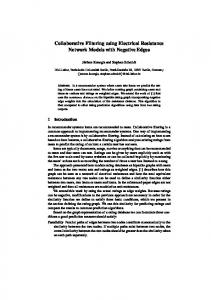
player responsible for the goal has kicked the ball is also registered. In this work the concept of ”goal opportunities” is created and consists of identifying the situations where an attacking player has a large probability of scoring a goal. The probability calculus is based on the position of the player (inside or outside the penalty area) and the number of players that he has in his view field aligned with the goal line. For each player this probability decreases by 0.2 plus 0.2 if the player is outside the penalty area. 3.1.4. Set Pieces A Set piece is an extremely important game situation [17] and can be divided as Corners, Goal-Kicks, Throw-Ins and Fouls. In this work all of these groups are detected, however, within the Fouls group, only offside situations are classified. 3.1.5. Ball Possession A soccer team has the possession of the ball in a given interval of time if, during that time, none of the players from the opposing team intercept the ball and the ball does not leave the playing field. To classify ball possession more succinctly, the soccer field was divided into twelve equal parts (six defensive and six offensives). Furthermore, a new concept was introduced which consists of evaluating the time a team takes to get to the last third of the field without losing the ball. This information is extremely relevant in order to classify the offensive style that a team uses during a game. This classification is divided into four levels: slow, medium, fast or break depending on when the opposing team recovers the ball. 3.2. Team Strategy Definition In this research two distinct high-level variables were used to increase the flexibility of our team strategy: Team Formation, relating to the players’ position on the field; and Set-Plays, a set of the players’ movements in combination. In order to define this information, the Playmaker tool[28] was used . This tool is comprised of two distinct modes: formation definition and set play definition. 3.2.1. Team Formation Team formation is defined by the positioning used by the players in order to occupy the field in the best possible manner. In this tool, the players’ positions are calculated through a Delaunay Triangulation [3] and a linear interpolation algorithm. For this task we used the same algorithm that was used in the Gouraud Shading algorithm [18], which simulates the differing light and color effects along a surface. The formation definition is based on the ball position. All ball positions included in the formation definition are used as vertices to create the triangulation. After determining the triangle (B1, B2, and B3) that encompasses the current ball position (B), player positions are calculated (P (B1), P (B2), and P (B3) are the players’ position when the ball is in the corresponding point). Figure 1 illustrates an example of the interpolation process [28]. 1. Calculate the I value (the intersection point between the line B1B and segment B2B3);
Figure 1. Gouraud Shading Interpolation
2. Calculate the interpolated target position regarding I as the current ball position and B2 and B3 as reference points (1): −−−→ | B2I | P(I) = P(B2) + (P(B3) − P(B2)) ∗ −−−→ −−−→ | B2I | + | B3I |
(2)
3. Calculate the new player position in relation to the ball position B (2): −−−−→ | B1B | P(B) = P(B1) + (P(I) − P(B1)) ∗ −−−−→ −−→ | B1B | + | BI |
(3)
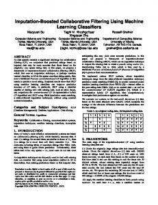
In this research, two distinct formations were defined (1-4-3-3 and 1-4-4-2) and 115 points were used for the definition of each formation. The experimental results showed that this type of approach is adequate for this context allowing a rich definition of a formation, relating the ball poistion with the players positions. An example of a 1-4-3-3 formation definition using the Playmaker tool is illustrated in Figure 2. 3.2.2. Set-Plays The Set-Plays definition can be seen as a flexible team plan for a specific game situation that can involve a specific game period, the number of scored goals, a game situation, such as a set piece, or even the opposing players’ position on the field. Normally, a Set-Play is identified by a name, a set of parameters (conditions) and players. Furthermore, a set play can be seen as a list of states. The possible transaction between these steps can be divided into three groups: (1) abort if not all the conditions to continue with the set play are met; (2) the next step transaction when all the conditions to continue are met; and finally (3) the finish transaction which indicates that a set play execution is completed. In this research 8 different set plays were used. They can be divided into four groups relating to a specific game situation. Only one SetPlay of each group was used in each simulation game. For each representative SetPlay figure the black and white line symbolizes the movement of the player and the ball respectively. It is important to note that
Figure 2. Example of 1-4-3-3 formation definition using the Playmaker tool
if, for some reason, the conditions for the realization of a Set-Play are not met it will be aborted: 1. Kick-off is a situation that characterizes the beginning or recommencement of a soccer match (e.g. after a goal is scored). In this work two set plays relating to this game situation were used: (a) Kick-off to winger constituted by 4 step (Figure 3)
Figure 3. Example of a Kick-off Set Play involving 4 steps
i. The kick-off taker passes the ball to the midfielder, while the defender positions himself to the left of the midfielder; ii. The midfielder passes the ball to the striker, while the winger moves nearer to the offside line to the left. The defender keeps himself to the left of the midfielder; iii. The striker passes the ball to the defender, while the winger keeps heading towards the offside line to the left; iv. The defender passes the ball to the winger. (b) Kick-off to winger constituted by 2 steps (Figure 4)
Figure 4. Example of a Kick-off Set Play involving 2 steps
i. The attacker makes a direct pass to the midfielder. The winger positions himself near the offside line to receive a pass from the midfielder; ii. The midfielder passes the ball to the winger. 2. Free Kick is a situation that occurs when a player violates the game play rules. For this situation, we have used two distinct set plays taking into account that it takes place in the offensive region, from our team’s perspective. (a) Free Kick direct to the goal (Figure 5) i. The taker passes the ball to a receiver near the goal; ii. The receiver shoots at the goal. (b) Free Kick where is privileged the ball possession (Figure 6) i. The taker passes the ball to the striker; ii. The striker passes the ball to the left-winger or to the right-winger; if this is not possible, he passes the ball back to the taker.
Figure 5. Example of a Free Kick Set Play direct to the goal
Figure 6. Example of a Free Kick Set Play where the ball possession is first priority
3. Goal Kick occurs when the ball has completely crossed the goal-line without a goal having been scored and having last been touched by an attacking team player. Two different Goal Kick plays were used: (a) Goal Kick constituted by 7 steps (Figure 7) i. The goalkeeper and the left defender move to the left region of the field (the left defender more to the left and in front of the keeper); ii. The goalkeeper kicks the ball to the region where the left defender is running. If the left defender intercepts the ball, the left midfielder moves to
Figure 7. Example of a Goal Kick Set Play involving 7 steps
the left and front of the left defender; iii. The left defender kicks the ball to the place where the left midfielder is running. If the left midfielder intercepts the ball, the left forward moves to the front and left of the midfielder; iv. The left midfielder kicks the ball to be intercepted by the left forward. A runner moves to the front of the left forward; v. The left forward kicks the ball forward to be intercepted by the runner; vi. The runner kicks the ball to his right and it is received by a kicker. The runner keeps running forward; vii. The kicker kicks the ball in a left and forward direction to be intercepted by the runner. (b) Goal Kick constituted by 3 steps (Figure 8) i. The players position themselves in two rows perpendicular to the goal line and in front of the penalty area (except the goalkeeper who stays inside the penalty area). The goalkeeper kicks the ball to the player closest to him on his right; ii. The player that has the ball, passes it to the player in front of him (on the other row) and slightly ahead of him (it is a zig zag slalom); iii. The next step is repeated until the last player receives the ball. 4. Corner Kick is awarded when the whole of the ball passes over the goal line without a goal being scored, and it was last touched by a player from the defending team. Two corner kick situations were used: (a) Corner Kick to the left striker (Figure 9) i. The taker passes the ball to the nearest receiver; ii. The receiver passes the ball to the left striker who is in front of the opponents goal;
Figure 8. Example of a Goal Kick Set Play involving 3 steps
Figure 9. Example of a beginning corner set play
iii. If the left striker has space to shoot, he will shoot at the goal, if not he passes the ball to the center striker; iv. The center striker receives the ball and shoots. (b) Corner Kick i. The taker passes the ball to the nearest receiver; ii. The receiver dribbles the ball back to the middle of the penalty box; iii. The receiver passes the ball to either the left, right or center striker; iv. Whoever receives the ball shoots at the goal;
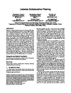
4. Methodology We describe the general idea of our approach to solve the given problem, i.e., the recommendation of a strategy for our team, given the way the opponent is playing. The idea is to select the strategy that has obtained the highest average of goal differences from past games where the opponents have played as our current opponent is playing. Or, using a different language, our two goals are: to locally rank the strategies by decreasing order of the average goal differences, and to select the top one. In the next section we describe in detail our approach divided in two phases: online and offline. Then, we present the main algorithms used. 4.1. Project Architecture Details This approach has two distinct phases: offline and online (Figure 10).
Figure 10. Project Architecture (where GD: Goal Difference; SIV: Selected Input Variables; SVM: Support Vector Machine)
The offline phase has 5 steps: 1. Simulation: it consists of developing a tool that automatically calculates the final game statistics through a log file selection (previously explained) [2]. It is important to note that, for this approach, all of the log files of the 2D simulation league between 2006 and 2009 were used. 2. Feature Selection: it uses the MARS algorithm [16] [32] to select the statistics that most influence the final game results (using the difference between the goals scored as a target) from an initial set of 60 final game statistics. This step is fully described in [1]; 3. Clustering: it groups the data calculated in step 1 into K clusters (only using the statistics selected in step 2). It uses the K-means algorithm. Since clustering algorithms are sensitive to the existence of irrelevant features, step 2 is crucial in order to enhance clustering results. 4. Training Classifier: it trains a classifier that can predict the group that best characterizes a given input data. Three different classification algorithms were tested: Support Vector Machines (SVM), Bagging and Random Forest (RF) because they
present consistently good results in a benchmark study [25] that compares 17 state-of-the-art classifiers on 21 datasets. 5. Selection of the Best Strategy per Cluster: defines the expected best strategy for a group of opponents with similar behavior, i.e., from the same cluster. The best strategy is the one with the maximum average of goal differences. To choose the best strategy per cluster, the following criteria were used in a sequential manner until only one strategy was selected: (a) Pick up the one with the maximum average goal differences from the FC Portugal team’s perspective; (b) Pick up the one that appears the most in each cluster; (c) Pick up the one with the maximum value for the evaluation MARS function. The online phase is made up of 2 steps: 6. Prediction: it predicts the most similar cluster to the given data. The model used for prediction was trained in step 4; 7. Assignment of the Best Strategy: it assigns the expected best strategy for a particular style of play by the opponent. For this, we have used the predicted cluster (obtained in the previous step) and the best strategy per cluster (step 5) in order to obtain the strategy that maximizes the average of goal differences for a given runtime input data. Further information about the different steps will be included in the Experimental Results section. Finally, it is important to note that all the data processing in this project was performed using the R software version 2.11.0 5 . 4.2. Multivariate Adaptive Regression Splines (MARS) Friedman’s 1991 Multiple Adaptive Regression Splines (MARS) model [16][32] employs recursive partitioning to locate product spline basis functions of an adjustable degree, rather than constants. This results in smooth adaptive function approximation as opposed to the crude steps or plateaus provided by regression trees. The method also takes into consideration splines involving interactions between previously selected variables so it can orient its basis functions other than on the original data axis. To aid interpretation, model terms are collected according to their inputs and their influence is reported in an ANOVA manner. The effects of individual variables and pairs of variables are collected together and graphically presented as function plots. MARS also employs cross-validation, prunes terms after over-growing, and can handle categorical variables. MARS builds its models according to Eq. (4) where the aim is to add together the weight of basis functions Bi (x) (ci are constant terms). k
bf ∑ ci Bi (x)
(4)
i=1
The construction of the MARS models is divided into two distinct phases: the forward and the backward passes. In the forward pass the algorithm starts with a model, 5 More
information available at http://www.r-project.org/
which only consists of the intercept term. After that, and being a greedy algorithm, it will include in the model the basis functions pairs that give the maximum reduction for the sum-of-squares residual error. Each new basis function consists of a term, already in the model, multiplied by a new hinge function, which is defined by a variable and a knot. This addition continues until the maximum number of terms is reached or if the change in the residual error is negligible. In order to generalize the model produced in this phase, the backward pass consists of pruning the model. It will remove terms one by one until the best sub model is reached and this is evaluated by the GCV (Generalized Cross Validation) measure variable. The result of MARS is an interpretable equation. The features used in the equation are the ones that are selected to explain the target variable. Since the MARS algorithm uses the recursive partitioning algorithm [10], this approach to selecting features is similar to the one described in [12]. 4.3. K-Means Algorithm Data clustering or Q-analysis or Typology or Clumping or even Taxonomy (depending on the applied field [19] appeared for the first time in 1954 [20]). One of the possible definitions of cluster analysis can be found at Webster [20] ”a statistical classification technique for discovering whether the individuals of a population fall into different groups by making quantitative comparisons of multiple characteristics”. Clustering algorithms can be divided into two groups: Hierarchical and Partitional [20]. The Hierarchical algorithm works in two ways: (1) it starts by agglomerating all of the data in the same cluster and recursively dividing the cluster into small clusters (divisive mode); or (2) it starts to put each data point in respective clusters and merges the most similar clusters in a hierarchical cluster (agglomerative mode). On the other hand, the Partitional algorithm does not impose a hierarchical structure and finds all the clusters iteratively. It starts by partitioning the data randomly and by redefining the partitions at each iteration according to the minimization of a given distance measure. Normally, due to the nature of the available data, the Partitional algorithms were preferentially selected. One of the most famous/adopted Cluster Partitional, due to its simplicity, efficiency and empirical success, is the K-Means algorithm. Over the years it has been used in several areas. The first work dates back to the 1950s [33]. It does not use a target field and this algorithm tries to uncover patterns in the set of input fields. It tries to group data in different sets (designated as clusters) according to their similarities. 4.4. Bagging The bagging algorithm is constituted by three distinct steps. The first step consists in generate Xk bootstrap samples (i.e., samples with replacement) of size n from an original dataset (with the same size). After that, the algorithm will train a predictor (tree) for each generated sample (the number of trees is typically 50-100 times [7][8], a value given by the Xk input parameter of the algorithm). Finally and, depending of the problem nature, the final result is the most predicted class by its base-classifiers (majority voting).
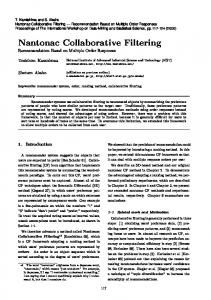
4.5. Random Forest Created by Breiman [9] Random Forest instantly became a commonly used method, mainly due to its simplicity (in terms of training and tuning) and performance [37]. Similar to the previously analyzed algorithm, Random Forest constructs a given number of trees. However, during the construction of each tree, at each node v variables are randomly selected (considering v ¡ number of input variables) and the best split in these v variables is used to split the node. At the end, the most voted class, by the set of trees in the forest is the predicted class (for more details see [9]). 4.6. Support Vector Machines (SVM) Based on the concept of decision planes that define decision boundaries, SVMs were developed by Vapnik [38], for binary classification. This technique tries to find the optimal separating hyperplane between two classes by maximizing the margin between the classes’ closest points (Figure 11).
Figure 11. SVM Classification (linear separable case)
The points lying on the boundaries are called support vectors and the middle of the margin is our optimal separating hyperplane. To construct an optimal hyperplane, SVM employs an iterative training algorithm which is used to minimize an error function. A more complete overview can be found in Vapnik [38] and Boser et al. [6].
5. Experimental Results In this section all the achieved results obtained in the two project phases (online and offline) will be described.
5.1. The Offline Phase
With regards to Figure 10, the first step of our approach was to develop a framework capable of automatically calculating the final game statistics through RoboCup 2006-2009 2D Simulation League log files. An exhaustive description about this step is available in [27] [2]. Step (2) consists in the identification of a subset of the calculated statistics (60) that most influence the game result and for that we used the MARS algorithm. However, we have started standardizing the data (Eq. 5 - where µ(x) is the sample average and σ (x) is the sample standard deviation) based on a previous work developed by Abreu et al. [1]. That work had two main goals: to select a feature subset in order to avoid irrelevant features that can decrease the performance of the clustering algorithm (step 3) and obtain an evaluation function that is used in step 7. For this reason the MARS and the RReliefF algorithms were tested and at the end MARS had a minor mean squared error (for more details please consult Abreu et al. [1]).
x=
x − µx σx
(5)
Consequently, in step (2) we used the MARS algorithm to discover the final games statistics that most influenced the games results (using as a target the difference of scored goals). The obtained expression is shown in Eq. 6. This expression includes variables relating to the total number of bad passes (BadPassTot), Pass Chains (PassChainTot), outside situations (OutTot), number of goals (GaolsTot), number of attacks (AttTot) and, finally, the statistics relating to ball possession per zones (1-LBposs-Def, 2-MBposs-Def, 3-RtBposs-Att etc.). The following measures are used to evaluate the MARS function: the coefficient of determination (RSq) which measures the quality of adjustment, the generalized coefficient of determination (GRSq) that measures how well the next value can be predicted using the structural part of the model and the past values of the residuals. The GRSq and RSq values vary between 0 and 1 (as higher the better).
f(x) = 3.85 + 1.51 ∗ max(0, BadPassTot − 75) +0.09 ∗ max(0, 75 − BadPassTot) −1.53 ∗ max(0, BadPassTot − 70) +0.34 ∗ max(0, BadPassTot − 62) +1.04 ∗ max(0, GoalsTot − 2) −1.62 ∗ max(0, 2 − GoalsTot) −0.16 ∗ max(0, 10 − OutTot) +2.29 ∗ max(0, Goalkick − 3) −1.62 ∗ max(0, Goalkick − 2) +0.95 ∗ max(0, O f f int − 2) −2.02 ∗ max(0, 2 − FastAtt) −0.71 ∗ max(0, AttTot − 6) −1.20 ∗ max(0, 6 − AttTot) +0.76 ∗ max(0, AttTot − 9) −10.2 ∗ max(0, 0.13 −0 1 − LBposs − De f 0 ) −29.2 ∗ max(0, 0.14 −0 2 − LBposs − De f 0 ) −2.45 ∗ max(0, 0.55 −0 1 − MBposs − De f 0 ) −32.5 ∗ max(0, 0.17 −0 2 − MBposs − De f 0 ) −6.03 ∗ max(0, 0.23 −0 4 − MBposs − Att 0 ) −2.88 ∗ max(0,0 3 − RBposs − Att 0 − 0.29) −8.81 ∗ max(0, 0.29 −0 3 − RBposs − Att 0 ) +0.30 ∗ max(0, PassChainTot − 13) −0.24 ∗ max(0, PassChainTot − 7) GRSq : 0.7827846RSq : 0.8317884
(6)
Having this previous knowledge as a base, the input of the system consists of three robotic teams’ binaries that occupied distinct positions in the final classification table (RoboCup 2009 2D league) in order to have a high spectrum of final game simulation results. Following this, 32 distinct team strategies (16 set plays combinations plus 2 formations) were defined and, in order to avoid outliers, each team used the same tactic in 10 simulations. As such, we simulated 480 games (3 teams x 16 strategies x 10 simulations). Using the obtained subset of statistics, the data instances are then grouped according to their similarity (step (3)). For that, we have used the K-means algorithm. In order to determine the optimal number of k clusters is (the optimal number of cluster is a compromise between the minimum sum square errors and the minimum number of clusters), the GAP algorithm was used. According to Tibshirani et al. [36] the number
that maximized the GAP should be used as the number of clusters (in our case this value was 9). In step (4) and according to the guidelines presented in Meyer et al. [25] three data mining methods (SVM, Random Forest and Bagging) were trained for the prediction of the cluster that would best characterize the data input (using as target the identifier of the k clusters produced in the previous step). In the training process a 10-fold Cross Validation was used and more than 1920 log files, including matches of the RoboCup 2D simulation league between 2006 and2009 were also used. With reference to the percentage rate in the test set of the 10-fold cross validation (previously described), SVM is the one that presents the highest result (96,4%), followed by RandomForest (93,59%) and Bagging (80,15%). In step (5) the expected best strategy (combination of Set Play and Formation) was defined according to the one that obtained best results in past games where the opponents were playing as our current opponent is playing (this step ends the offline phase). 5.2. The Online Phase For step (6), the SVM model generated in step(4) was used to predict the cluster where each game (input data) is expected to be more similar to (the duration of this process is 10 cycles). Finally, in step (7), the expected best strategy was assigned according to cluster predicted in step(6). To produce experimental results for the online components, 840 games were simulated (280 per opponent team) between FC Portugal and each of the following teams : Wright Eagle, Nemesis and Bahia 2D. In that simulation, the online (OL) phase was executed using different frequencies in a simulated robotic soccer with 6000 cycles: every 500 cycles (OL500), every 1000 cycles (OL1000) and every 2000 cycles (OL2000) - a simulated robotic soccer has 6000 cycles. These three configurations were compared with a Baseline algorithm, which is an approach that chooses the strategy that FC Portugal will use before the game and, during the game it does not make any changes. The results were evaluated according to the number of wins, draws and defeats (Table 3 and 5 illustrated those achievements). If, for some reason, there was a draw between the results produced by at least two algorithms (same number of victories, defeats and draws), a draw scale was used. This scale consisted of assigning 4 points for a victory, 2 points for a draw and 1 point for a loss. These values increased 0.1 per goal scored (increasing with the difference of goals scored in case of victory and decreasing in case of defeat). For instance, if FC Portugal wins two games by the difference of 2 or 12 goals, these games will be ranked with 4.2 and 5.2 points respectively. On the other hand, if this team loses two games by the difference of 2 or 12 goals, these games will be ranked with 0.8 and -0.2 points respectively (this scale was used to measure the team’s performance in Table 2). The comparison is done using the Friedman rank test. We have compared the average of the results of each of the three configurations plus the baseline approach (four different options). The 280 simulations per opponent team were divided into 4 distinct groups (one per option). The ranks obtained are shown in Table 1. The null hypothesis of equivalence between the four predictors is rejected with a p-value of 0.00000303. Comparing the three configurations against the baseline for a 5% significance level with the BonferroniDunn test [14], we have obtained CD = 1.2617. CD is the critical value for the difference of mean ranks between the baseline and any other of the three predictors. It is proved that OL500 and OL2000 are better than the baseline.
Table 1. Ranks of the Friedman test for the online mode 1
2
3
4
5
6
7
8
9
10
11
12
Mean
Baseline
4
4
4
4
4
3
3
4
4
3
4
2
3,58
OL500 OL1000 OL2000
2 1 3
2 3 1
2 1 3
2 3 1
2 1 3
1 4 2
1 4 2
3 2 1
1 3 2
1 4 2
2 1 3
1 3 4
1,67 2,50 2,25
5.3. Performance Improvements Regarding the scale presented above (Table 2), we were able to improve the FC Portugal team’s performance by over 35% (35,87%, 35,31% and 35,34%) for the three used online frequencies. Doing a more deep analysis concerning the opponent (using the same scale), for the Nemesis team, every OL configurations beat the baseline approach (always more than 135% of improvement). The FC Portugal team presented a smaller improvement against the Bahia 2D (around 28%). This result is explained by the fact that Bahia team is a rookie in the RoboCup competition and, because of that, teams like FC Portugal normally win the games scoring many goals and for that reason the improvement will always be a little bit limited (comparing to the others two teams). Table 2. Percentage of FC Portugal Performance Improvement using a pre defined scale as criteria
Baseline
Score by Opponent OL500 OL1000
OL2000
Percentage by Opponent OL500 OL1000 OL2000
WE
120.8
165.2
161.5
159
37.58%
33.77%
31.62%
Nemesis Bahia
78.8 1051.4
188.8 1344.7
188.6 1342.5
186.5 1347.6
139.59% 27.90%
139.34% 27.69%
136.68% 28.17%
Total
1251 Total Percentage
1699.7 35.87%
1692.7 35.31%
1693.1 35.34%
Regarding to the number of wins, defeats and draws (Table 3), the three OL approaches presented outstanding results. In global terms (without individual team analysis), the OL500 increased the number of wins by 25,78%, decreased the number of losses by 7,34% and also decreased the number of draws by 51,72%. In what concerns to OL1000, it presented an increase of wins of 24,44%, a decrease of defeats of 7% and an also a 48,28% decrease in the number of draws. Finally, to OL2000, it presented an increase of wins (25,55%) and a decrease of 6,31% and 68,87% for defeats and draws respectively. Finally, in what concerns to the difference of goals scored (always from the FC Portugal perspective), the numbers presented were also excellent: 98,45%, 98,79% and 98,38% for the OL500, OL1000 and OL2000, respectively (Table 5), which constitutes an admirable result, when comparing to other studies, such as that by Stone et al. [34], which presented an increase of 9 scored goals in average and that by Ledezma et al. [24], that increased in average one scored goal (in one hundred games). In conclusion it is proved without any doubts that our approach is capable to improve a performance of a robotic simulated soccer team.
Table 3. Percentage of FC Portugal Performance Improvement using the number of victories, defeats and draws as criteria Baseline
OL500
OL1000 Victory/Defeat/Draw
OL2000
WE
0/277/3
Nemesis Bahia Total
1/276/3 224/33/23 225/586/29
1/274/5
0/278/2
1/278/1
2/269/9 280/0/0 283/543/14
0/267/13 280/0/0 280/545/15
1/271/8 280/0/0 282/549/9
Total
25.78%/-7.34%/-51.72%
24.44%/-7.00%/-48.28%
25.33%/-6.31%/-68.97%
Percentage
Table 4. Percentage of FC Portugal Performance Improvement using the difference of scored goals as criteria
Baseline
Score by Opponent OL500 OL1000
OL2000
Percentage by Opponent OL500 OL1000 OL2000
WE Nemesis
-1619 -2069
-1217 -1073
-1204 -1061
-1249 -1042
24.83% 48.14%
25.63% 48.72%
22.85% 49.64%
Bahia
790
2245
2230
2244
184.18%
182.28%
184.05%
Total
-2898 Total Percentage
-45 98.45%
-35 98.79%
-47 98.38%
Table 5. Percentage of FC Portugal Performance Improvement using the difference of scored goals as criteria
Baseline
Score by Opponent OL500 OL1000
OL2000
WE Nemesis Bahia
-1619 -2069 790
-1217 -1073 2245
-1204 -1061 2230
-1249 -1042 2244
Total
-2898 Total Percentage
-45 98.45%
-35 98.79%
-47 98.38%
Percentage by Opponent OL500 OL1000 OL2000 24.83% 48.14% 184.18%
25.63% 48.72% 182.28%
22.85% 49.64% 184.05%
6. Conclusions and Future Work In this research, an approach capable of constructing an online team model was presented. From a soccer team coach perspective it is important to obtain all possible knowledge relating to how the opponent plays. Such knowledge can be used to prepare new games (offline phase) or to adapt the strategy used along the game (online phase). Focusing on these two phases, the main goal of this research is to prove that if a coach agent during the game periodically changes his team strategy using the knowledge previously generated in the offline phase, it is possible to improve his team’s performance. We based our strategy in two very simple premises – two team formations and 8 different set plays – and proved that it is possible to increase the team’s performance. As outlined in the previous section, SVM proved to be the best algorithm in the prediction step (step (4)). Additionally, OL500 and OL2000 proved to be better than a baseline approach to increase FCPortugal performance (step (7)). The obtained results were very promising and the team’s performance increased by 35.87% and 35.4% using the OL500 and OL2000, respectively. If we executed an opponent individual analysis, for the Nemesis team, the performance of our team improved by more than 135% in each tested case. For the top tournament team (Wright Eagle), the improvement was of 37,58% for OL500 and 31,62% for OL2000. Also, establishing
a comparison between other literature works, none of the analyzed works presented results as promising as those presented in this paper. They simply increased the number of scored goals (by an average of 1 [24] or 9 [34]). This problem is an example of a much more generic type of problems (as described in the Problem Formulation section). We believe that the approach we presented can be used in many different environments such as health treatment strategy selection where it is very important to identify the best strategy to eliminate/control a disease throughout proliferation markers/hormonal receptors status or in transport planning to select planning options such as bus/train frequency in order to optimize the general quality of the service (e.g minimize delays). The presented framework can be used for problems with a finite number of strategies. Both x and y variables (as described in the Problem Generalization section) assume continuous values in soccer environment. However, the used framework could be easily extended for non numerical variables by: (1) using a different distance function in clustering when x has non-numeric variables (see step (3) in Figure 10) and/or (2) using a different criterion (such as the mode instead of the average, for instance) to rank strategies when y is non-numeric (step (5) in Figure 10).
Acknowledgment This project was partially supported by project Knowledge Discovery from Ubiquitous Data Streams (PTDC /EIA-EIA/098355/2008).
References [1]
[2]
[3] [4] [5] [6] [7] [8] [9] [10] [11] [12] [13]
P.H. Abreu, D.C. Silva, J. Mendes-Moreira, L.P. Reis and J. Garganta, Using multivariate adaptive regression splines in the construction of simulated soccer teams’ behavior models. Computing science technical report, Faculty of Engineering of University of Porto, Rua Dr. Roberto Frias, s/n 4200-465 Porto PORTUGAL. Available at http://www.fe.up.pt/ pha/article.pdf, 2010. P.H. Abreu, J. Moura, D.C. Silva, L.P. Reis and J. Garganta, Performance analysis in soccer: a Cartesian coordinates based approach using RoboCup data. Soft Computing - A Fusion of Foundations, Methodologies and Applications, 16(1), 47-61, 2011. H. Akiyama and I. Noda, Multiagent positioning mechanism in a dynamic environment. RoboCup 2007: Robot Soccer World Cup XI, Lecture Notes in Computer Science, 5001, 2008, 377-384. R. Aler, J. Valls, D. Camacho and A. Lopez, Programming robosoccer agents by modeling human behavior. Expert Systems with Applications, 36(2) (2009), 1850-1859. C. Bauckhage, C. Thurau and G. Sagerer, Learning humanlike opponent behavior for interactive computer games. In Pattern Recognition, 2781, 148-155, Springer, 2003. B. Boser, I. Guyon and V. Vapnik, A training algorithm for optimal margin classifiers. In COLT ’92: Proceedings of the fifth annual workshop on Computational learning theory, 144-152, ACM, 1992. L. Breiman, Bagging predictors. In Machine Learning, 24(2) (1996), 123-140. L. Breiman, Arcing classifiers. The Annals of Statistics, 26(3)(1998), 801-849, 1998. L. Breiman, Random forests. Machine Learning, 45 (2001), 5-32. L. Breiman, J. Friedman, R. Olshen and C. Stone, Classification and Regression Trees. Wadsworth and Brooks, Monterey, CA, 1984. J. Brown and R. Burton, Diagnostic models for procedural bugs in basic mathematical skills. Cognitive Science, 2(2) (1978), 155-192. C. Cardie, Using decision trees to improve case-based learning. In In Proceedings of the Tenth International Conference on Machine Learning, 25-32. Morgan Kaufmann, 1993. S. Chee, J. Han and K. Wang, RecTree: An Efficient Collaborative Filtering Method. Proceedings of the Third International Conference on Data Warehousing and Knowledge Discovery, 141-151, 2001.
[14] [15] [16] [17] [18] [19] [20] [21] [22] [23]
[24] [25] [26]
[27]
[28] [29] [30] [31] [32] [33] [34]
[35] [36] [37] [38] [39]
[40] [41]
J. Demsar, Statistical comparisons of classifiers over multiple data sets. Journal of Machine Learning Research, 7, 1-30, 2006. C. Druecker, S. Huebner, H. Neumann, E. Schmidt, U. Visser and H. Weland, Virtu-alweder: Using the online-coach to change team formations. Technical report, University of Bremen, 2000. J. Friedman, Multivariate adaptive regression splines (with discussion). Annals of Statistics, 19, 1-141, 1991. J. Garganta, J. Maia and F. Basto, Analysis of goal-scoring patterns in European top level soccer teams. Science and Football III (Edited by T. Reilly, J. Bangsbo and M. Hughes), 246-250, 1997. H. Gouraud, Continuous shading of curved surfaces. In IEEE Transactions on Computers, 20(6) (1998), 87-93. A. Jain and R. Dubes, Algorithms for clustering data. Prentice-Hall, Inc., Upper Saddle River, NJ, USA, 1988. A. K. Jain, Data clustering: 50 years beyond k-means. Pattern Recognition Letters, 31(8) (2010), 651666. H. Kitano, M. Asada, Y. Kuniyoshi, I. Noda and E. Osawa, Robocup: The robot world cup initiative. In Working Notes of IJCAI Workshop: Entertainment and AI/Alife, 19-24, 1995. H. Kitano, M. Asada, Y. Kuniyoshi, I. Noda and E. Osawa, Robocup: The robot world cup initiative. In AGENTS ’97: Proceedings of the first international conference on Autonomous agents, 340-347,1997. Y. Kuniyoshi, M. Inaba and H. Inoue, Learning by watching: Extracting reusable task knowledge from visual observation of human performance. IEEE Transactions on Robotics and Automation, 10 (1994), 799-822. A. Ledezma, R. Aler, A. Sanchis and D. Borrajo, Predicting opponent actions by observation. In RoboCup2004, 286-296, Springer, 2004. D. Meyer, F. Leisch and K. Hornik, The support vector machine under test. Neurocom-puting, 55(1-2) (2003), 169-186. G. Paliouras, V. Karkaletsis, C. Papatheodorou and C. Spyropoulos, Exploiting learning techniques for the acquisition of user stereotypes and communities. In UM99 User Modeling: Proceedings of the Seventh International Conference, 169-178. Springer Verlag, 1999. J. Portela, P.H. Abreu, L.P. Reis and J. Garganta, An intelligent framework for automatic event detection in robotic soccer games: An auxiliar tool to help coaches improving their teams performance. In ICEIS 2010, 244-249, 2010. L.P. Reis, R. Lopes, L. Mota and N. Lau, Playmaker: Graphical definition of formations and setplays. In CISTI 2010, 582-587, 2010. P. Resnick and H. Varian, Recommender systems. Communications of the ACM, 40(3) (1997), 56-58. P. Riley, M. Veloso, M. and G. Kaminka, Towards any-team coaching in adversarial domains. In AAMAS-02, 1145-1146, 2002. C. Sammut, S. Hurst, D. Kedzierand and D. Michie, Learning to fly. In ICML92, 385-393, 1992. S. Sekulic and B. Kowalski, Mars: A tutoria. Journal of Chemometrics, 6(4) (1992), 199-216. H. Steinhaus, Sur la division des corp materiels en parties. Bull. Acad. Polon. Sci, 1, 801-804, 1956. P. Stone, P. Riley and M. Veloso, Defining and using ideal teammate and opponent agent models. In Proceedings of the Twelfth Innovative Applications of Artificial Intelligence Conference, 1040-1045, 2000. X. Su and T. Khoshgoftaar, A Survey of Collaborative Filtering Techniques (Review Article). Journal of Advances in Artificial Intelligence (2009), 1-19. R. Tibshirani, G. Walther and T. Hastie, Estimating the number of clusters in a dataset via the gap statistic. Royal Statisticcal Society B, 63(2) (2001), 411-423. H. Trevor, R. Tibshirani and J. Friedman, The elements of Statistical Learning: Data Mining, Inference, and Prediction. Springer Series in Statistics. ISBN:978-0-387-84857-0, 2009. V. Vapnik, The Nature of Statistical Learning Theory (Information Science and Statistics). Springer, 2nd edition, 1999. G. Webb and M. Kuzmycz, Feature based modeling: A methodology for producing coherent, dynamically changing models of agents competencies. User modeling and user-adapted interaction, 5(2) (1996), 117-150. G. Webb, B. Chiu and M. Kuzmycz, Comparative evaluation of alternative induction engines for feature based modeling. International Journal of Artificial Intelligence in Education,8 (1997), 97-115. G. Webb, M. Pazzani and D. Billsus, Machine learning for user modeling. User Modeling and User-
[42]
[43]
Adapted Interaction, 11(1-2) (2001), 19-29. G-R. Xue, C. Lin, Q. Yang, W. Xi, Yu. Z, H-J and Z. Chen, Scalable collaborative filtering using clusterbased smoothing. Proceedings of the 28th annual international ACM SIGIR conference on Research and development in information retrieval, 114-121, 2005. SH.Yang, B. Long, A. Smola, H. Zha and Z. Zheng, Collaborative competitive filtering: learning recommender using context of user choice. In Proceedings of the 34th international ACM SIGIR conference on Research and development, 295-304, 2011.