Using model transformation for generating visualization ... - CiteSeerX

Using Model Transformation for Generating Visualizations from Repository Contents An Application to Software Cartography Technical Report TB 0601

Alexander M. Ernst, Josef Lankes, Christian M. Schweda, André Wittenburg

Software Engineering for Business Information Systems (sebis) Ernst Denert-Stiftungslehrstuhl Chair for Informatics 19 Technische Universität M¨ unchen Boltzmannstraße 3, 85748 Garching b. M¨ unchen, Germany {ernst, lankes, schweda, wittenbu}@in.tum.de November 2006

Abstract

Documenting application landscapes, a central part of Enterprise Architecture Management, heavily relies on graphical and intuitive visualizations. Planning, deciding, and controlling in respect to measures on the application landscape all benefit from such diagrams. In our research project Software Cartography we have analyzed a multitude of visualizations, originating from several major industrial users. Thereby, we found that the majority of diagrams used is created manually, a tendency we could confirm in a survey on Enterprise Architecture Management Tools. We regard the manual creation of these visualizations leading to significant disadvantages, mainly due to reasons of creation effort and modeling rigor. Therefore, we view the availability of an automatic process for generating well-formed diagrams as essential to Enterprise Architecture Management. This work presents an approach for leveraging model transformations to automatically generate graphical representations of application landscapes. An object oriented model for describing these visualizations is presented, which is augmented with formal definitions forming a basis for automated diagram layouting. We put this findings into practice and describe an exemplary layouting approach employing a genetic algorithm solving an optimization problem. Thus, we want to make a contribution to the visualization in Enterprise Architecture Management.

c TU M¨

unchen, sebis, 2006. All rights reserved.

II

Contents

0 Preface

1

1 Motivation: Visualizing Application Landscapes

2

2 Generating Software Maps using Model Transformation Techniques 2.1 Relationship between Semantic and Symbolic Models . . . . . . . . . . . 2.2 Model Transformation and Software Maps . . . . . . . . . . . . . . . . . 2.2.1 Leveraging Model Transformation for Generating Software Maps 2.2.2 Introducing a Visualization Model . . . . . . . . . . . . . . . . . 2.2.3 Introducing Transformation Rules . . . . . . . . . . . . . . . . .

. . . . .

. . . . .

. . . . .

5 6 9 10 11 13

3 Software Map Types 3.1 Software maps with a base map for positioning . . 3.1.1 Cluster Map . . . . . . . . . . . . . . . . . 3.1.2 Process Support Map . . . . . . . . . . . . 3.1.3 Interval Map . . . . . . . . . . . . . . . . . 3.2 Software maps without a base map for positioning 3.3 The Layering Principle . . . . . . . . . . . . . . . .

. . . . . .

. . . . . .

. . . . . .

. . . . . .

. . . . . .

. . . . . .

. . . . . .

. . . . . .

. . . . . .

. . . . . .

. . . . . .

. . . . . .

. . . . . .

. . . . . .

. . . . . .

15 15 16 17 18 19 19

4 Visualization Model 4.1 Object-oriented Visualization Model . . . 4.1.1 Map Symbols . . . . . . . . . . . . 4.1.2 Visualization Rules . . . . . . . . . 4.2 General Formalization of the Visualization 4.2.1 Prerequisites . . . . . . . . . . . . 4.2.2 Visualization Objects - Definition . 4.2.3 Map Symbols - Definition . . . . . 4.2.4 Map Symbols - Auxiliary concepts 4.2.5 Map Symbols - Examples . . . . . 4.2.6 Visualization Rules - Definition . . 4.2.7 Visualization Rules - Examples . . 4.3 Mitigations of the Visualization model . .

. . . . . . . . . . . .

. . . . . . . . . . . .

. . . . . . . . . . . .

. . . . . . . . . . . .

. . . . . . . . . . . .

. . . . . . . . . . . .

. . . . . . . . . . . .

. . . . . . . . . . . .

. . . . . . . . . . . .

. . . . . . . . . . . .

. . . . . . . . . . . .

. . . . . . . . . . . .

. . . . . . . . . . . .

. . . . . . . . . . . .

. . . . . . . . . . . .

21 23 25 27 33 33 34 37 40 42 44 46 51

c TU M¨


. . . . . . . . . . . . Model . . . . . . . . . . . . . . . . . . . . . . . . . . . . . . . .

. . . . . . . . . . . .

III

CONTENTS

4.4

4.3.1 Mitigations of planar map symbols . . . 4.3.2 Mitigations of linear map symbols . . . Concretization of the Visualization Model . . . 4.4.1 Concretizations for planar map symbols 4.4.2 Concretizations for linear map symbols

. . . . .

. . . . .

. . . . .

. . . . .

. . . . .

. . . . .

. . . . .

. . . . .

. . . . .

. . . . .

. . . . .

. . . . .

. . . . .

. . . . .

. . . . .

. . . . .

. . . . .

52 57 57 58 62

5 Related Work

66

6 Outlook

68

A Planar map symbol area homomorphism

71

B Multiplicity values formalized

73

C From symbolic model to optimization problem

76

c TU M¨


IV

CHAPTER

0

Preface

The research project Software Cartography, which started in February 2003, establishes methods and models for documenting, evaluating, and planning application landscapes and especially defines notations as well as visualization techniques utilizing concepts from the field of conventional cartography [HGM02]. Sponsors and partners of the research project are AMB Generali, Allianz, AXA, BMW Group, Deutsche Börse Systems, Deutsche Post, Ernst Denert-Stiftung, K¨ uhne + Nagel, HVB Systems Information Services, M¨ unchener R¨ uck, sd&m, Siemens, Siemens Business Services, T-Com, and TUI. Thanks to our sponsors and partners!

c TU M¨


1

CHAPTER

1

Motivation: Visualizing Application Landscapes

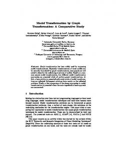
Application landscapes are complex systems consisting of hundreds or even thousands of business application systems. They are a major investment of modern enterprises and are subsequently changed to support new or changed business goals, business strategies, and business processes. The documentation, evaluation, and planning of these application landscapes are major challenges of enterprises, especially when seen in the context of increasing the alignment of business and information technology. In the research project Software Cartography, we made an initial analysis on different types of visualizations and interviewed various stakeholders about their concerns on the application landscape [MW04, LMW05c]. One of the findings was, that nowadays many of the visualizations are created manually by positioning symbols on a canvas. This is a task, which is both time consuming and error-prone, even if a repository based tool ensures data consistency with the actual information about the application landscape. Our approach is meant to support automatic generation of such visualizations. The absence of a standard for modeling application landscape as well as the diversity of concerns expressed by the stakeholders of the application landscape has lead to a high number of different visualization types, varying in the information displayed therein and in the concepts employed for displaying. The analysis further showed that a certain kind of flexibility regarding the usage of different symbols is neccessary, especially if the visualizations should be adapted to suite the needs of stakeholders interested in highlighting aspects of the application landscape. This flexibility, which is of course available when creating visualizations manually, should not be pruned by automatic generation. To give a short introduction on the visualizations this report focuses on, Figure 1.1 shows an exemplary visualization of the application landscape, called a software map. This software map is assembled like a matrix, in which the business processes make-up the x-axis and organizational units make-up the y-axis. Positioning a rectangle in the matrix means that this

c TU M¨


2

1. Motivation: Visualizing Application Landscapes

Acquisition

Warehousing

Distribution

Customer Relationship Management System (2100)

Headquarter Subsidiary Munich

Monetary Transaction System (Germany) (300)

Price Tag Printing System (Germany/ Munich) (1700)

Online Shop (100)

POS System (Germany/Munich) (1600) Monetary Transaction System (Germany) (300)

Campaign Management System (1500)

Subsidiary Hamburg

Price Tag Printing System (Germany/ Hamburg) (1720)

Inventory Control System (200)

Subsidiary London

Monetary Transaction System (Great Britain) (350)


Price Tag Printing System (Great Britain) (1750)

POS System (Great Britain) (1650)

Monetary Transaction System (Germany) (300)

Warehouse

POS System (Germany/ Hamburg) (1620)

Customer Complaint System (1900)

Monetary Transaction System (Great Britain) (350)

Product Shipment System (Germany) (400)

Legend Map Symbols B (1)

C

Visualization Rules

Business Process A

A

Business Application B with Id 1 Organizational Unit C

C

Vertical Alignment

A

„A“ is supported by „B (1)“ and used at „C“

Horizontal Alignment B (1)

Figure 1.1: Example software map showing the dependencies between business processes, business applications, and organizational units

specific business application supports the business processes to which the rectangle is aligned on the x-axis and is used by the organizational unit to which the rectangle is aligned on the yaxis. This relationship between business processes, business applications, and organizational units can be seen as a ternary relationship, which is discussed in detail in chapter 3. Furthermore stretching the rectangle for a business application in either x- or y-direction refers to the fact that the business application supports either more than one business processes or is used by more than one organizational unit. From Figure 1.1 it can e.g. be derived that the business application ’Monetary Transaction System (Germany)’ supports the business processes ’Acquisition’ and ’Distribution’. The supporting system for the ’Acquisition’ process is used by the organizational units ’Headquarter’, ’Subsidiary Munich’, ’Subsidiary Hamburg’, and ’Warehouse’ and the support function for the ’Distribution’ process is used by the organizational units ’Subsidiary Munich’ and ’Subsidiary Hamburg’. It can also be derived from Figure 1.1 that the organizational unit ’Subsidiary London’ uses a different business application ’Monetary Transaction System (Great Britain)’ to support the business processes ’Acquisition’ and ’Distribution’. By now, hardly any tool available on the market is capable of generating such visualizations using a predefined visualization scheme from data stored in a repository, as discussed in the ’Enterprise Architecture Management Tool Survey 2005’ [se05]. This coheres with the lack of standardized ways of visualizing application landscapes. Existing standards like the Unified Modeling Language (UML) [OM05b] developed by the Object Management Group (OMG) are used to visualize the architecture of a single business application and are usually not suitable for displaying the whole application landscape. The concepts of UML do not match with the concepts needed to document an application landscape [MW04, LMW05c]. Information elements like organizational units, etc. as well as visualization elements needed

c TU M¨


3

1. Motivation: Visualizing Application Landscapes

to build Figure 1.1 are not known by UML. A further problem arising from this situation characterized by manually drawn diagrams is that the visualizations have no well-defined semantics that determines, which graphical symbol in the visualizations refers to which semantic element in the repository. This leads to visualizations, which may only be interpreted correctly by the author of the drawing. Therefore, managing a major investment by drawing figures, which cannot be interpreted correctly, is quite problematic: ’Drawing is no management!’ [Ri05]. The following chapters show our approach to conveniently and flexibly generate software maps using the well known concept of model transformation (see chapter 2). The approach is designed to offer both flexibility in visualization definitions and a strict definition of what the visualization concepts signify. In chapter 3 we give a summary of the main requirements on software maps and will introduce the types of software maps we have identified so far. Chapter 4 presents the central part of our approach, the visualization model, defined informally using an object-oriented model and formally using mathematical terms. Before we give an outlook in chapter 6, related approaches for solving similar problems are discussed in chapter 5.

c TU M¨


4

CHAPTER

2

Generating Software Maps using Model Transformation Techniques

The motivation in chapter 1 stated that today, software maps are often created manually. Tools employed to create software maps can be distinguished into two groups, the nonrepository-based tools like Microsoft Visio or Microsoft PowerPoint and the repository-based tools like ARIS Toolset (from IDS Scheer AG) or Corporate Modeler (from Casewise, Inc.)1 . The non-repository-based tools do not provide out of the box functionalities to create software maps, e.g. Microsoft Visio stencils providing shapes and rules for drawing software maps. Existing stencils for Microsoft Visio, e.g. the ArchiMate [JLL06] stencil, provide basic functionality for modeling software maps, but some problems still prevail: • Other stencils, which are not part of the methodology, can be used. This softens the given methodology by enabling the user to add symbols, which are not part of the methodology, resulting in drawings without defined semantics. • The stencils do not directly support positioning-related concepts such as alignment, which is e.g. used in Figure 1.1 to show a support/use-relationship between business processes, business applications, and organizational units. • Non-repository-based tools do not use an information model, which defines the semantics of elements, their attributes, and relationships to other elements. A correspondent information model for Figure 1.1 would define the three elements business process, organizational unit, and business application. All elements would have an attribute ’name’ and a ternary relationship ’supports’ would connect the three elements (see chapter 3 for further explanations)2 . 1

For further tools utilized to create software maps refer to the ’Enterprise Architecture Management Tool Survey 2005’ [se05]. 2 Of course, this does not comprise definitions what concepts like business process etc. exactly are. Therefore, an additional glossary is needed.

c TU M¨


5

2. Generating Software Maps using Model Transformation Techniques

Munich

Hamburg

Garching

London

Online Shop (100)

Human Resources System (700)

POS System (Germany/Munich) (1600)




Monetary Transactions System (Great Britain) (350)


Monetary Transactions System (Germany) (300)

Business Traveling System (1000)

Worktime Management (Germany/Munich) (1800)

Fleet Management System (900)


Data Warehouse (800)


Customer Satisfaction Analysis System (2000)

Accounting System (500)

MIS (1300)


Document Management System (1100)

Worktime Management (Germany/ Hamburg) (1820)

Supplier Relationship Management System (1200)


Costing System (600)

Financial Planning System (1400)



Worktime Management (Great Britain) (1850)

Legend Map Symbols A

Location A

Visualization Rules A

„A“ hosts „B (1)“ and „C (2)“ B (1)

B (1)

Business Application B with Id 1 C (2)

nesting

Figure 2.1: Exemplary cluster map showing which business application is hosted at which location

The repository-based tools either have a predefined information model or provide the possibility to create or adapt the information model. However, the ’Enterprise Architecture Management Tool Survey 2005’ [se05] showed that the visualization concepts of such tools are still lacking some capabilities, especially concerning flexible and automated generation of software maps. To clarify the problems arising during the creation of software maps, we explain the differences between a semantic model and a symbolic model in the following section 2.1, using the software map shown in Figure 2.1 as a running example. The differentiation of the semantic and the symbolic model is also a key concept behind our approach for software map generation.

2.1

Relationship between Semantic and Symbolic Models

Figure 2.1 shows a software map, which is of the type Cluster Map 3 , showing which locations host which business applications. The business application ’Online Shop (100)’ for example is hosted at the location ’Headquarter’. To gain a more in depth understanding of the software map in Figure 2.1, we outline how we re-engineered four models that address different aspects of the software map. These four models, described in the following paragraphs, led us to our approach for software map generation. Creating a semantic model, containing the information of the software map, and an information model, representing the metamodel, results in the UML object and class diagrams in Figures 2.2 and 2.3 if an object-oriented notation is chosen. The object diagram in Fig3

For a description of software map types see chapter 3.

c TU M¨


6


: hostedAt OnlineShop : BusinessApplication

Munich : Location

: hostedAt Monetary Transaction System (Germany) : BusinessApplication : hostedAt Accounting System : BusinessApplication

Location

: hostedAt

BusinessApplication

hosted at

name : String

Costing System : BusinessApplication

1

name : String *

id : Integer

: hostedAt Product Shipment System (Germany) : BusinessApplication

Hamburg : Location : hostedAt

Fleet Management System : BusinessApplication

Figure 2.2: Semantic model of the cluster map in Figure 2.1

Figure 2.3: Information model of the cluster map in Figure 2.1

ure 2.2 visualizes parts4 of the semantic model and each object in the diagram represents an information object (e.g. the location ’Munich’, the business application ’Human Resources System (700)’). The properties of the information objects, not visualized in Figure 2.2, are the values the attributes of an object, e.g. the value ’Munich’ for the name of the location Munich and ’100’ for the id of the business application ’Online Shop’. The information model in Figure 2.3 is the metamodel on which the semantic model is based, it consists of • the two classes Location and BusinessApplication, • the attribute name for both classes, • an attribute id for the class BusinessApplication, and • an association hosted at. Beside the class diagram the semantics of the elements (classes, attributes, associations, etc.) has to be specified, which can for example be done in a glossary in a textual way or more formally, if e.g. specific use cases call for this. An entry in such a glossary for the class BusinessApplication may be: A Business Application is a software system with a minimum of one user and a database to store information. Further, a business application has to support at least one business process. More semantic information may be retrieved from the visualization, if e.g. the gray background color of the locations also has a semantics. In our example all semantic information is covered by the class diagram in Figure 2.35 . Beside the semantic model and the information model we can also derive a symbolic model and a visualization model from the software map in Figure 2.1, which are also modeled using UML object and class diagrams are shown here. The symbolic model (Figure 2.4) shows what 4

The whole semantic model is too large for a figure in this report, because each symbol in Figure 2.1 must be represented by an object, resulting in an object diagram with 34 objects. 5 It has to be noted that re-engineering a software map can only be done with the creator of the map if no information model and/or legend does exist.

c TU M¨


7


: intersecting Online Shop : Rectangle

: Nesting : intersecting

Monetary Transaction System (Germany) : Rectangle

: Nesting

: intersected : intersected

Accounting System : Rectangle

: Nesting : Nesting

x : Real y : Real

: intersected

: intersecting Costing System : Rectangle

inner

Rectangle Munich : Rectangle

: intersecting

1

* Nesting

width : Real

: intersected

height : Real backgorundColor : Color : intersecting Fleet Management System : Rectangle

borderColor : Color

: intersected : Nesting

Hamburg : Rectangle

: intersecting Product Shipment System (Germany) : Rectangle

: Nesting

: intersected

Figure 2.4: Symbolic model of the cluster map in Figure 2.1

1

*

text : String outer

Figure 2.5: Visualization model of the cluster map in Figure 2.1

symbols a visualization consists of and what demands and constraints exist regarding their positioning. The visualization model (Figure 2.5) is the metamodel of the symbolic model, specifying what kinds of symbols can be used in a visualization and what constraints can be imposed to their positioning. The only kind of symbol used in Figure 2.1 is a rectangle, which also provides a text-field and is called Rectangle in the visualization model in Figure 2.5. In addition there exists a positioning constraint, which is expressed by a visualization rule, in the software map. This visualization rule, which is represented in the visualization model by the class Nesting, meaning that a symbol is nested inside another symbol, is used to represent the association hosted at (see Figure 2.3). An additional visualization rule PlanarNonIntersection, which defines that two specific symbols may not intersect, is not contained in Figure 2.5 due to readability issues and will be introduced in chapter 4. The visualization objects of the symbolic model, which are modeled as objects in Figure 2.4, are instances of classes from the visualization model in Figure 2.5 and correspond to the symbols used in Figure 2.1. The attributes of each object are not shown in Figure 2.4, e.g. the object Munich:Rectangle has the attribute value ’Munich’ for the attribute text and the attribute value ’gray’ for the attribute backgroundColor. In the research project Software Cartography we call symbols like Rectangle map symbols 6 and the variables of each symbol, e.g. the backgroundColor attribute, are called visual variables 7 . The rules in a visualization, e.g. the ’Nesting’, are called visualization rules 8 . These three terms are adopted from cartography(see [HGM02] and [Sl03]). Further map symbols, visual variables, and visualization rules are introduced in section 2.2. Section 4 develops formal definitions of the terms in the context of Software Cartography and automated visualization generation. After having retrieved the four models from the visualization we gain a deep understanding of the software map and know which information should be contained in the map: Figure 2.1 shows, which business application is hosted by which location using rectangles with a gray background color for locations and rectangles with a white background color for business applications. The hosting relationship is expressed in Figure 2.1 by nesting a rectangle for a business application inside a rectangle for a location. 6

in German Gestaltungsmittel in German Gestaltungsvariable 8 in German Gestaltungsregel 7

c TU M¨


8


Munich

Hamburg

Garching

London

Online Shop (100)

Human Resources System (700)

POS System (Germany/Munich) (1600)




Monetary Transactions System (Great Britain) (350)


Monetary Transactions System (Germany) (300)

Business Traveling System (1000)

Worktime Management (Germany/Munich) (1800)

Fleet Management System (900)


Data Warehouse (800)


Customer Satisfaction Analysis System (2000)

Accounting System (500)

MIS (1300)


Document Management System (1100)

Worktime Management (Germany/ Hamburg) (1820)

Supplier Relationship Management System (1200)


Costing System (600)

Financial Planning System (1400)



Individual Software

Worktime Management (Great Britain) (1850)

Legend Map Symbols A

Visualization Rules

Location A

A

„A“ hosts „B (1)“ and „C (2)“ B (1)

B (1)

Business Application B with Id 1 C (2)

nesting

Figure 2.6: Cluster map with an additional map symbol

A problem, which we have often been confronted with in practice, are visualizations without such a defined information model, visualization model, and a connection between these models, defining what information is expressed by which visualization concept. Either all or some of the models and their connection are not documented, neither with class diagrams nor in a textual way, or models are defined but not applied correctly. If e.g. the modeling tool allows adding further elements to a visualization without having them properly connected to information in the semantic model, visualizations such as in Figure 2.6 can be created. In Figure 2.6, the rectangle with a red colored dotted border has no connection to any element in the semantic model (see Figure 2.2). This gap leads to a visualization, of which the information can neither be interpreted correctly nor be stored in a repository in an accessible and maintainable way. This is because the information model defines the structure for the information and the information that some systems are ’Individual Software’ is not intended here. The argumentation above shows that a tight link between the information model and the visualization model is needed to guarantee consistency between the the information (semantic model) in the repository and the visualization (symbolic model). The following section 2.2 presents our approach to ensure this consistency.

2.2

Model Transformation and Software Maps

Model transformation is a technique to translate one or more source models into one or more target models. In software engineering, model transformation is used in many different ways. For example, E/R models are transformed to SQL statements capturing the data definition language for a database schema or, for example, UML class diagrams are transformed to Java source code. An OMG recommendation using model transformation in software engineering

c TU M¨


9


is the Model Driven Architecture [OM01] (MDA)9 . In case of the MDA, a Platform Independent Model (PIM) might be a UML class diagram or a set of diagrams, which are using only concepts on a highly abstract level without being platform specific, where being not platform specific means that the PIM makes no assumptions about the implementation platform and is technology-neutral. For example a PIM which models a software system might be independent of a specific programming language and can be transferred to a model using Java, C++, or SQL which is then the Platform Specific Model (PSM), using concepts of the specific platform. A PIM might use a concept named String, which would be transferred into a Java-PSM concept java.lang.String or a SQL-PSM concept VARCHAR(20). The concepts for transforming a PIM-String to a concept in a PSM vary depending on the platform. In the case of SQL additional information that the string has a maximum length of 20 characters is also needed, since SQL only supports a string with a given maximum length. Therefore, information might have to be added during the transformation. In addition the transformation in our example has to specify how a metamodel concept from the PIM is transferred to a metamodel concept of the PSM. If the PIM is modeled using UML class diagrams the transformation to Java will transform a UML class to a Java class, whereas a transformation to SQL may transform a UML class to a SQL table definition.

2.2.1

Leveraging Model Transformation for Generating Software Maps

The idea of transforming models is used in automated generation of software maps to tighten the link between the semantic model and the symbolic model. Transforming an element of a semantic model (e.g. Accounting System:BusinessApplication10 ) to an element of a symbolic model (e.g. Accounting System:Rectangle) can be performed by a set of rules. One rule may state that every business application is transformed to a rectangle with text using a white background color. The concepts of model transformation used for generating software maps are shown in Figure 2.7. Beside the concepts semantic model, information model, symbolic model, and visualization model, which have been introduced in section 2.1, a Metamodel and a Transformation are introduced. The Metamodel is the common language for the information model and the visualization model. As the semantic model with its information objects is an instance of the information model, the information model itself is an instance of a metamodel, likewise the visualization model is. The common metamodel for the information model and the visualization model simplifies the requirements for the Transformation, because if no common metamodel exists, the transformation must also transform one metamodel into the other metamodel. The transformation sketched in Figure 2.7 is meant to be a bidirectional transformation, which is expressed by the arrow showing to the semantic and the symbolic model. A bidirectional transformation provides the possibility to create visualizations by transforming a semantic 9

It has to be noted that a semantic model and a symbolic model cannot be compared to a CIM, PIM, or PSM. The concepts PIM and PSM refer to a dependency on a platform. Semantic and symbolic models do not deal with platform dependencies. 10 The notation A:B means the object A is an instance of the class B.

c TU M¨


10


Transformation Semantic Model

Symbolic Model

is instance of based on Information Model BusinessApplication hosted at 11

0..* 0..*

id : Integer nameEnglish : String nameGerman : String status : Enumeration

1

has version

0..*

0..*

0..*

supports

1..*

Visualization Model

BusinessApplicationVersion id : Integer v ersionId : Integer status : String plannedFrom : Date plannedTo : Date inDev elopmentFrom : Date inDev elopmentTo : Date inProductionFrom : Date inProductionTo : Date inRetirementFrom : Date inRetirementTo : Date

OrganizationalUnit id : Integer nameEnglish : String nameGerman : String plzPoBoX : String city : String country : String address : String

is instance of based on

modifies

ABC

0..*

used at

BusinessProcess 0..*

SupportRelationship child

id : Integer nameEnglisch : String nameGerman : String description : String isPrimary : Boolean lev el : Integer

0..*

superprocess

0..1

parent

next

Project

0..*

id : Integer nameEnglish : String nameGerman : String startDate : Date endDate : Date selected : Boolean

previous 0..1

0..1

based on

predecessor

is instance of

is instance of

based on

based on

Metamodel e.g. Meta Object Facility (MOF) 2.0

Figure 2.7: Model transformation techniques in software map generation

model to a symbolic model and also to change the semantic model by interacting with the visualization11 . An important requirement on the metamodel is that all concepts needed for conveniently modeling information and visualization models and also for a straightforward expression of the transformation with the help of a suitable language or approach, are supported by the metamodel. In the case of leveraging model transformation for generating software maps, we propose an object-oriented metamodel for the information model and the visualization model. Buckl [Bu05] showed that the assumption of an object-oriented metamodel like the Meta Object Facility (MOF) [OM06a] is sufficient for information models [Ha04, La05, Br05a] commonly in use in the domain of Software Cartography. That the assumption of an visualization model using MOF concepts also holds, is shown in chapter 4. Furthermore, a common metamodel simplifies the transformation, since both models are using the same language. A transformation rule stating that each BusinessApplication is transformed to a Rectangle (see above) needs a mechanism to create rectangles with text for each business application. In MOF, this can be performed using the Factory allowing to create new Elements.

2.2.2

Introducing a Visualization Model

The goal of using model transformation for the generation of software maps is to provide a flexible approach for generating visualizations. Furthermore, the transformation ensures that the semantic and the symbolic models fit to each other. Some possible elements of an information model have been introduced in section 2.1, e.g. a business application or a business process. Elements of the visualization model are for example rectangles, circles, and lines, called map symbols. Other important elements of the 11

In this report we only cover the direction from semantic to symbolic model.

c TU M¨


11


Name

Symbol

Rectangle

Name

Visual Variable

Background color

Ellipse

Border color

Chevron

Line size

Cylinder

Line type

Line Table 2.1: Examples for map symbols

Table 2.2: Example for visual variables

Name

Example

Visualization Rule B A B

XSequence

Chevron for process A is to the left of chevron for process B

A

PlanarNonIntersection Rectangle for application A does not overlap with rectangle for application B Nesting

Rectangle for application A is nested in the rectangle for organizational unit B

Alignment

Rectangle for application A is positioned under the chevron for process B A

Attachment

Line representing a data stream is attached atA the rectangles for applications A and B

A

A

B

A A B B A B A A A A B BB B A

B B

A

A

AB B B A

B A B B B A A

A B B A B B A A A B A B

B A B A

BB

B

Table 2.3: Examples for visualization rules visualization model are the visualization rules, which define constraints on map symbols, mostly regarding their positioning, i.e that one symbol is nested inside of another symbol. To leverage the idea of using model transformation for generating software maps a visualization model is needed, which covers all visual concepts used on software maps. Tables 2.1 and 2.2 show some examples for map symbols and different values for visual variables. The rules relating map symbols geometrically are exemplified in Table 2.3. As currently no common language for describing these symbols and rules exists (see chapter 5), it is yet not directly possible to describe the visualizations in another manner than a quite informal textual or example driven way. If a higher level of preciseness shall be achieved, a more formal description for visualizations is needed. Such a more formal way has to satisfy several requirements, e.g. it has to be precise enough to act as a basis for automatic creation of maps and it has to be easy to understand in order to keep it simple in use. Chapter 4 gives a comprehensive overview of theses requirements and introduces a visualization model, which contains elements sufficient for addressing visualization as described in section 3.

c TU M¨


12


rule OrgUnit2Rectangle { from infoObject : Semantic.OrganizationalUnit to symbol : Symbolic.Rectangle ( text = infoObject.name, backgroundColor = #CCCCCC ) ) rule BusinessApp2Rectangle { from infoObject : Semantic.BusinessApplication to symbol : Symbolic.Rectangle ( text = infoObject.name || "(" || infoObject.id || ")" ), rule : Symbolic.Nesting ( inner = symbol, outer = transforming (infoObject.hostedAt) ) ) Figure 2.8: Exemplary transformation rule set

2.2.3

Introducing Transformation Rules

The missing part to complete the generation of software maps via model transformation are the transformation rules. Transformation rules on the level of models (information model and visualization model ) can formally express the graphical notation of the application landscape in the context of a viewpoint12 . These rules do not only map certain information model classes, e.g. BusinessApplication to visualization model classes, e.g. Rectangle; they can further contain predicates and expressions used to filter the information to be transformed, thus hiding concepts not of importance in the particular viewpoint. The transformation rules can then be used to transform information objects and their semantic relationships to visualization objects and their positioning relationships. A simple example for a transformation rule generating the software map in Figure 2.1 by transforming the semantic model in Figure 2.2 to the symbolic model in Figure 2.4 may be the rule set13 in Figure 2.8. The first rule OrgUnit2Rectangle transforms each information object, which is an instance of the class OrganizationalUnit, to an instance of Rectangle. In addition, the text field is set to the name of the information object and the background color is set to gray (#CCCCCC). The second rule transforms each business application to a Rectangle, setting the text field to a combination of the name and the id of the business application. Furthermore, instances of the 12 13

Viewpoint in terms of the IEEE Std 1471-2000 [IE00, LMW05a]. The transformation rules are expressed using pseudo-code.

c TU M¨


13

2. Generating Software Maps using Model Transformation Techniques : intersecting Online Shop : Rectangle

: Nesting : intersecting

Monetary Transaction System (Germany) : Rectangle

: Nesting

: intersected : intersected

Munich : Rectangle

: intersecting Accounting System : Rectangle

: Nesting

: intersected

: intersecting Costing System : Rectangle

: Nesting

r1

: intersecting

Fleet Management System : Rectangle

: intersected : Nesting

r2 Product Shipment System (Germany) : Rectangle

: intersected

R Hamburg : Rectangle

: intersecting : Nesting

: intersected

Figure 2.9: Excerpt of the symbolic model in Figure 2.4

wr 1 ⎛ w ⎞ − ⎜ xR − R ⎟ > 0 2 ⎝ 2 ⎠ hr 1 ⎛ hR ⎞ y r1 − − ⎜ yR − ⎟>0 2 ⎝ 2 ⎠

xr1 −

wR ⎛ w ⎞ − ⎜ xr1 + r1 ⎟ > 0 2 ⎝ 2 ⎠ hR ⎛ hr1 ⎞ yR + − ⎜ y r1 + ⎟>0 2 ⎝ 2 ⎠

xR +

...

Figure 2.10: Inequality systems derived from the symbolic model in Figure 2.9

association hostedAt from a business application to an organizational unit are transformed to a instances of the class Nesting, which are respectively connected to the rectangle corresponding to the business application and the rectangle corresponding to the organizational unit. We are currently analyzing, whether model transformation languages like ATL [AT06], which resembles the pseudo-code in Figure 2.8, or other approaches, like automatically generated Java classes, fit the requirements for the transformation mechanism best. Assuming that the visualization model is sufficiently strictly defined and that there are sufficiently efficient (’computable’) ways of finding valid values for the visual variable (i.e. positions of the map symbol instances in most cases) the semantic model can be used to automatically generate a corresponding visualization. In chapter 4 we present such a strictly defined visualization model on which we build a mechanism that translates the problem of finding a suitable layout into an optimization problem. The constraints of the optimization problem, which results from the symbolic model in Figure 2.9, showing the symbolic model with the annotated rectangles R, r1, and r2, and parts of the resulting inequality system are shown in Figure 2.10. The target function of the optimization problem could e.g. be used to control aesthetic aspects as e.g. distances between map symbol instances. The complexity and kind of optimization problem depends on the type of the visualization rules to be employed. Therefore, special attention has to be payed to the solver used to solve the optimization problem (see chapter 4). The result of the calculations performed by the solver is positioning information, which can be used by a rendering engine to create visualizations.

c TU M¨


14

CHAPTER

3

Software Map Types

The automated view generation introduced in section 2 is based upon a method for the representation of application landscapes, the so-called software maps [LMW05c, LMW05b]. In this section the software maps are briefly introduced and basic graphical concepts behind the maps are identified. Based on this, chapter 4 outlines a comprehensive model of these concepts, which is suitable for describing the graphical buildup of software maps. This model constitutes a metamodel of the visualization for software maps and can therefore serve as a visualization model as mentioned in section 2. Similar to the concept of maps used in cartography, a software map is composed of a base map and several layers. While in the field of conventional cartography a visualization can rely on prominent topological characteristics, e.g. latitude and longitude, to derive the base map, no such characteristics exist in software cartography. Therefore, no single base map exists, suitable for building all different kinds of visualizations on. After having analyzed various software maps we have been able to derive different types of software maps, differentiated e.g. by the kind of base map they are utilizing: • Software maps with a base map for positioning - utilizing the concept of positioning map symbol instances to transport (formally) defined semantics • Software maps without a base map for positioning - performing ad-hoc positioning of the map symbol instances

3.1

Software maps with a base map for positioning

The main characteristic of these software map types is that an explicit meaning is assigned to the position of the map symbols present on the base map, i.e. the position has semantics. These software maps are further subdivided into three map types the cluster map, the c TU M¨


15

20,00

20,00

20,00

3. Software Map Types

Org. Unit 1

10,00

10,00

10,00

10,00

Org Unit 1.1

# 1 2 3 4

Business Application 1









Business

Figure 3.1: Excerpt from a cluster map Application 4 Graphical Concept Gray rectangle with label “Organizational unit *” White rectangle with label “Business Application *” Nesting of a rectangle as in 1 in a rectangle as in 1 Nesting of a rectangle as in 2 in a rectangle as in 1

Meaning Organizational unit called “*” Business application called “*” Organizational unit belongs to another organizational unit Organizational unit uses a business application

Table 3.1: Meaning of the graphical concepts in Figure 3.1 process support map, and the interval map, according to the layout of the base map and the information contained therein.

3.1.1

Cluster Map

The characteristic feature of a cluster map is that it utilizes the concept of nesting to visualize a relationship between the cluster element and the nested element, as it is shown in Figure 3.1. In this figure, the rectangle labeled Org. Unit 1.1 is nested within the rectangle labeled Org. Unit 1, whereas the small rectangles (with labels Business Applications 1, Business Applications 2, etc.) are all nested within the rectangle Organizational Unit 1.1. The nesting may e.g. visualize an use-relationship between an organizational unit and a business application, or a belongs to-relationship in the organizational chart, as detailed for the example from Figure 3.1 in Table 3.1. Therefore, Figure 3.1 shows that organizational unit 1.1 belongs to organizational unit 1, and e.g. that this organizational unit uses business application 1.

c TU M¨


16


Process 1 Process 1.1

Location 1


Location 2


Location 3

Process 1.2



Figure 3.2: Excerpt from a process support map

3.1.2

Process Support Map

The main graphical concept behind the process support map is the alignment of one map symbol in respect to another map symbol. Thereby, it is possible that a map symbol totally or partially overlaps another map symbol, in respect to its x-coordinate or also in respect to its y-coordinate. An example is shown in Figure 3.2 (Figure 1.1 depicts a complete exemplary process support map), where the rectangle labeled Business Application 1 overlaps with the chevron labeled Process 1.1 in respect to the x-coordinate and with the text box Location 1 in respect to the y-coordinate. Furthermore, in a process support map, the map symbols that are used as a reference for the alignment are always located at the edge of the map, forming two axes: a horizontal and a vertical one. The vertical axis is in most cases located at the left edge of the map, the horizontal one at the top. As it is often made up of map symbols representing processes [LMW05c], this software map type is called process support map. Thus, two kinds of map symbols on a process support map can be distinguished: the axis map symbols, which are part of the two axes of the map, and the aligned map symbols, which are aligned to the axes. The buildup of the axes suggested above leads to a major difference to axes as they are usually employed in coordinate systems. While the values denoted on a coordinate axis are commonly continuous attributes, the axes of a process support map convey discrete attributes, as there is only a finite number of axis map symbols on each axis. The exemplary process support map in Figure 3.2 visualizes information that conforms to the information model (metamodel) shown in Figure 3.3. Thereby, the concepts described in this information model are visualized by the graphical concepts of the process support map as follows: • A business process-instance is visualized as a chevron, these chevrons are also used to build a x-axis, thereby they are ordered as indicated by the predecessor -relationships of the business business process-instance they represent. If a business process-instance is a subprocess of another business process-instance, the respective chevrons are shown

c TU M¨


17


predecessor

0..1 BusinessApplication used at

id : Integer name : String

1

SupportRelationship

*

*

1 used from

- next

0..1 - previous

BusinessProcess id : Integer name : String *

* 0..1

- child

- parent

used at 1 OrganizationalUnit

superprocess

id : Integer name : String

Figure 3.3: Relationship between organization unit, business process and business application

below the parent process. • Each of the boxes forming the y-axis is used to visualize one organizational unit-instance. In this case, an arbitrary ordering is used. • Each business application-instance is visualized by one or more rectangles, which are the aligned map symbols of the process support map. For each supports relationshipinstance, a rectangle representing the business application-instance indicated by the association end supports is shown, and this rectangle is aligned to the chevron representing the supported business process and the rectangle representing the location where this business process is supported (in the context of the respective supports relationship). Thus, it can e.g. be deduced from Figure 3.2 that Business Application 1 supports Process 1.1 at Location 1 and that Business Application 2 supports the same process Process 1.1 at Location 2. When considering the objects that can be assigned to an axis in a process support map, it has to be distinguished whether the objects are ordered or not. If these objects are linearly ordered, it is possible and advantageous to order the map symbol instances representing these objects, leading to the concept of an ordered axis. If there is no order established on the objects (or such a relation exists, but is not used), the objects can nonetheless be used to form an axis, although the ordering of the axis map symbols is arbitrary then. This may e.g. be utilized to optimize the aesthetics or map space consumption of the visualization.

3.1.3

Interval Map

An interval map consists of similar types of map symbols as the process support map described above, axis map symbols and aligned map symbols. The characteristic difference is that at least one of the axes visualizes a continuous attribute. As such an axis is able to convey information about an interval scaled attribute [Fa99] without losing information, this software map type is called interval map. Taking the concept time as the continuous attribute is very common for these interval maps [LMW05c], which is then in most cases visualized on the horizontal axis. The at-

c TU M¨


18


2006 Jan Business Application 1

Feb

Mar

Apr

May

Jun

Jul

Aug

Sep

Oct

Nov

v 1.5

Dec

Jan

v 2.0

v 1.5 v 2.0 v 2.5

v1.0


Figure 3.4: Excerpt from an interval map

tribute displayed on the vertical axis varies from usage context to usage context, but mostly, a discrete attribute is used. As with the process support map, the attribute values for an instance represented by an aligned map symbol are visualized by alignment with certain areas of the axes. Thereby, a prominent aspect is visualizing time spans, as for example in Figure 3.4. By placing the rectangle labeled v1.5 below the interval of the horizontal axis that ranges from January to December, the following is expressed: the version v1.5 has been in existence from January to December1 . Aligning in respect to the horizontal axis determines the corresponding business application Business Application 1.

3.2

Software maps without a base map for positioning

The second category of software maps, the software maps without a base map for positioning, does not use positioning of the map symbols on the base map to convey information to the viewers, which means that the position of these symbols can be changed without affecting the meaning of the visualization. Concepts affecting the positioning of map symbols transport an explicit meaning only on the layers above the base map, e.g. a traffic light positioned in the upper right corner of a symbol expresses a relationship between the information object visualized and the measure visualized by the traffic light. ‘

3.3

The Layering Principle

The layering principle, exemplified in Figure 3.5, has been adopted from (geographic) cartography [Sl03]. It constitutes a basis for selective visualization of information in software maps. As it is possible to display various types of information (population density, average income, etc.) on the topographic base map of a geographic map, additional information can also be visualized on the base maps defined by the software map types described above. In 1

For further explanations of the colors of the rectangles, see [LMW05b].

c TU M¨


19

Feb

Mar

Apr


Measures Interconnections Applications Base Map

Figure 3.5: Layers of a software map

Figure 3.5, a cluster map - base map is used and on top of this base map, e.g. connections between business applications or some measures (visualized by pie charts) can be displayed. Arranging such additional information in layers yields two main benefits: • As the layers can be ordered, it becomes clear which map symbol instances are above which other map symbol instances, i.e. cover which map symbol instances. • More important, the layers can be specifically shown and hidden, making selective information visualization possible. Thus, the layering principle is an instrument suitable to hide complexity, which is unnecessary in a given usage context.

c TU M¨


20

CHAPTER

4

Visualization Model

Chapter 2 identified a visualization model as an integral part of sebis’ approach to software map generation and chapter 3 presented in detail the visualizations that should be covered by such a model. Now, a visualization model consisting of visualization concepts that fulfill the requirements arising from the demands specified (like map symbols and visualization rules) is introduced. Visualization objects, e.g. map symbol instances, are formally defined here, in terms of this visualization model. Additionally the model is constructed to fulfill specific requirements arising from the way this kind of model is meant to be used (see chapter 2). According to those requirements a visualization model should be • sufficiently easy to understand in order to be a helpful tool in specifying software maps, • sufficiently strictly defined in order to be a basis for automated visualization generation, • sufficiently flexible in order to leverage the introduction of new map symbols and visualization rules, • sufficiently adaptable in order to enable improvement of the automated layouting without having to redesign the basic structure of the model, and • sufficiently efficiently calculable in order to ensure the existence of time efficient (and perhaps memory efficient) algorithms for creating software maps. As the demands stated above span different levels of abstraction as well as different aspects of use, our approach abstains from a holistic and monolithic model to address all of them in an adequate way. Instead, the visualization model pursues a three tiered approach, as shown in Figure 4.1. The topmost level of the model (the Object-oriented Visualization Model ) is formed by an object-oriented representation of the visualization concepts suggested above (i.e. map symbols c TU M¨


21

4. Visualization Model

Object-oriented Model of Visualization Concepts

General Mathematical Closure Formalization and Filling

Simplification Proofs

Properties

Concrete Closure Definition

Concretization of Visualization Rules for Concrete Closure

Specific Map Symbols

Concretization of Visualization Model

Concretization

Further Mathematical Definitions of Visualization Concepts

General Visualization Model

Object-oriented Visualization Model

Figure 4.1: Three-tiered structure of the visualization model and visualization rules), which is described more detailed in section 4.1. This representation strongly depends on the Meta Object Facility 2.0 (MOF) [OM06a] and can therefore conveniently be described utilizing class diagrams, which themselves constitute a well-known way of providing information about the general structure of an object-oriented model to an user. Despite the obvious advantages of such a representation, MOF was not intended for and hence does not provide sufficient capabilities for describing the exact nature of visualization concepts (their graphical semantics) in an unambiguous way. The second level of the model (the General Mathematical Formalization), formed by mathematical and logical terms and expressions, is therefore introduced to complement the objectoriented description by an exact mathematical description of the respective visualization concepts. This mathematical description utilizes both algebraic terms as well as terms from the predicate calculus in order to cover the different kinds of graphical representations and implications of the visualization concepts by a denotational semantics [Sc04]. Section 4.2 explains this mathematical description more in detail. Together, the object-oriented representation and its mathematical complement form the General Visualization Model. Due to the highly different languages used for expressing those two parts, one might think, that the General Visualization Model in fact decomposes into two models, just informally coupled. However, a quite formal way of coupling the two layers is possible, based on a formalization of the object-oriented constructs. Such a formalization is out of the scope of this article, thus referencing to considerable work already done in this field, e.g. by Broy [BCR06] or by Evans [Ev98], the latter one pursuing an approach utilizing the Z-notation [Sp92] that strongly bases on concepts of the predicate calculus. The demands for an easy to understand (class diagrams), strictly defined (mathematical definitions), and flexible (using object-oriented mechanisms to introduce new concepts) visualization model are full or in major parts already satisfied by the General Mathematical

c TU M¨


22


Visualization Model. The third level (the Mathematical Concretization) of our model is concerned with concepts ensuring the model to be efficiently calculable and adaptable, when concerning its calculation paradigm. The fulfillment of those demands strongly depends on constructs introduced in the General Visualization Model, such as the filling and the closure, which form a basis for an effectively and efficiently calculable concretization of this model. These concepts are introduced in section 4.3 and complemented by proven mitigations for visualization rules employing closures and fillings instead of the symbols concerned1 . The actual concretization of the General Visualization Model, which makes use of these concepts, is described in section 4.4. Thereby, the approach pursued through the concepts mentioned above separates the universally valid specification of the General Visualization Model from its possible concretizations, enabling the implementor to choose a concretization (and thus a mitigation of the universally valid concepts) that best suits his decision in the context of the calculation complexity vs. visualization optimacy trade-off. Hereby, the adaptability demanded is achieved. The General Visualization Model is not affected by any change in the selection of the simplifications made, only the concretization has to be changed, if desired due to optimizations regarding calculation speed or visualization aesthetics. The concretization contains information on how to translate instances of the visualization model concepts, e.g. into an optimization problem as subsequently described in section 4.4.1.

4.1

Object-oriented Visualization Model

As mentioned above, the object-oriented representation of the visualization concepts makes up the top level tier of the visualization model. In order to conveniently model the concepts on this tier, MOF [OM06a] and UML class diagrams (see [OM05a]) as a notation are subsequently used. Thus the classes displayed in the diagrams are instances of MOF:Constructs:Class. Thereby, we distinguish between a CoreVisualizationModel, which defines the basic concepts of the visualization model and extending packages, which have to be introduced to be able to describe visualizations in a way to fit specific application needs. Specific map symbols (such as a Rectangle or a Chevron) and visualization rules (such as Nesting or Ordering) can be added in these extending packages, which are thereby built upon the core package by importing it. For exemplary purposes, we introduce a SoCaVisualizationModel package here, which builds visualization rules and map symbols suitable for describing software maps as introduced in chapter 3 on the concepts of the core visualization model. Due to the genericity of the core visualization model, it is of course possible to use it as the basis of other visualization model packages, stressing again the exemplary nature of the SoCaVisualizationModel package, which, while being suitable for the maps introduced above, is certainly not without potential for further improvement. The package structure made up thereby is shown in Figure 4.2. Figure 4.3 introduces the core visualization model. Its basic classes and their meaning are explained here briefly: Diagram represents the model of a complete visualization, as exemplified in Figure 2.1. It 1

Proven mitigations here mean, that the fulfillment of certain rules on closures and fillings is proven to ensure the fulfillment of the rule on the corresponding map symbol instances.

c TU M¨


23


CoreVisualizationModel

«packageimport»

SoCaVisualizationModel

MapSymbols

ConstraintVisualizationRules

TargetVisualizationRules

Figure 4.2: Package structure of the visualization model is made up of the visualization objects that form the respective diagram. Packages that use the core visualization model may add meta-information (via attributes) as e.g. creator or users of the diagram. VisualizationObject represents an object of the kind that make up a diagram description and may be categorized into map symbols and visualization rules. MapSymbol represents a type of graphical element of which instances can be used in a visualization, e.g. a rectangle. An instance of a map symbol Rectangle, e.g. the concrete rectangle labeled Munich in Figure 2.1, is called a map symbol instance. VisualizationRule represents a type of restriction that can be imposed upon one or more instances of visualization objects, e.g. in respect to their placement or other aspects of their appearance in case of map symbols as suggested in section 3. An actual restriction is called a visualization rule instance. ruling represents a bidirectional association. It represents for a map symbol instance the union of all visualization rule instances that are connected to this map symbol instance. For a visualization rule instance, it returns all map symbol instances ruled (i.e. connected) by the respective rule instance. For purposes of software cartography, the concepts from the CoreVisualizationModel package are refined to a SoCaVisualizationModel package (see Figure 4.4) containing the following basic concepts: Real is a primitive type of which an instance a number from the set of real numbers (also denoted as R). Color is a primitive type representing color information. This type is explained in detail in section 4.2, whereas here the shorthanded explanation via the considerably different displaying capabilities of different drawing canvases is given, which have to be accommodated by an adequately abstract and hence flexible definition. c TU M¨


24


+ visObjects

Diagram 1

+ /ruled {union}

VisualizationObject

*

ruling

*

MapSymbol

VisualizationRule

+ /rules {union} *

LinearMapSymbol

PlanarMapSymbol

ConstraintVisualizationRule

TargetVisualizationRule

Figure 4.3: Object-oriented core visualization model (Package CoreVisualizationModel) SoftwareMap represents a specialization of Diagram, containing a creation date. MapSymbol is extended with an attribute zIndex that is used to determine, which map symbol instance is meant to be on top of which other and an attribute visibility that is used to determine, whether a particular map symbol instance is visible or not. PlanarMapSymbol is extended with an attribute borderColor representing the color of the borderline of the symbol, an attribute fillColor representing the color for filling inner parts of the symbol, an optional attribute text, representing the contents of a label included in the symbol and an optional attribute textColor, used to represent the color of the text in the label included in the symbol. LinearMapSymbol is extended with an attribute lineColor representing the color the linear map symbol instance is drawn with. Canvas is a specialization of MapSymbol, representing the drawing surface of a software map. All map symbols contained in the software map topdress the Canvas. This symbol is introduced especially for facilitating reflections over the overall properties of the software map, e.g. its dimension.

4.1.1

Map Symbols

Despite the rather intuitive distinction2 between linear and planar map symbols, as introduced above, a formal way of determining whether a symbol is planar or linear has to be backed by a mathematic understanding of the map symbol, which is here postponed until the mathematic description is established in section 4.2. Figure 4.5 shows parts of the structure of the SoCaVisualizationModel package. This packages imports the contents of the package CoreVisualizationModel. The classes MapSymbol, LinearMapSymbol, and PlanarMapSymbol in Figure 4.5 have already been extended in the SoCaVisualizationModel package shown in Figure 4.4. The attributes of the map symbol classes constitute the visual variables 3 (outlined in section 2.1) of the respective map symbol. A quick overview over the classes introduced in Figure 4.5 is given below: 2

This distinction is made as different types of rules apply to different types of map symbols: while it makes sense to ask, whether something is inside an area (planar map symbol instance), it does not make sense to ask,

c TU M¨


25


Diagram

+ visObjects

VisualizationObject

* + /ruled {union}

1

ruling

*

MapSymbol

*

VisualizationRule

zIndex : Integer

+ /rules {union}

visibility : Boolean

PlanarMapSymbol

SoftwareMap creationDate : Date

LinearMapSymbol

borderColor : Color

lineColor : Color

ConstraintVisuali zationRule

TargetVisuali zationRule

fillColor : Color text : String [0..1]

1

textColor : Color [0..1]

1

«primitive»

«primitive»

Real

Color

Canvas width : Real

+ canvas {subsets visObjects}

height : Real

Figure 4.4: Package SoCaVisualizationModel

MapSymbol zIndex : Integer visibility : Boolean

PlanarMapSymbol

LinearMapSymbol

borderColor : Color

lineColor : Color

fillColor : Color text : String [0..1] textColor : Color [0..1]

Chevron x : Real

Ellipse

Rectangle

y : Real

x : Real

x : Real

inset : Real

y : Real

y : Real

width : Real

semiX : Real

width : Real

x : Real [2..*]

height : Real

semiY : Real

height : Real

y : Real [2..*]

Polyline

Figure 4.5: Package SoCaVisualizationModel::MapSymbols

c TU M¨


26


Ellipse is a map symbol representing an elliptical shape and is defined via the position of its center (x and y) as well as via the attributes representing the length of its respective semiaxes (semiX and semiY). Such elliptical shapes may e.g. be used for visualizing business objects or organizational units in a similar fashion as in Event Driven Process Chains [Sc01]. Rectangle is a map symbol representing a rectangular shape and is defined via the attributes representing center (x and y) as well as via attributes representing the lengths of the sides (width and height). Such shapes may be used for e.g. representing information objects or functional areas. Chevron is a map symbol representing a special kind of polygon and is defined via the attributes representing center (x and y) as well as via attributes representing the lengths of the sides (width and height). It furthermore employs an additional variable, the inset, for describing the distance of the bendpoint in the vertical lines from the rectangular line. This symbol is for example used for representing a business process as shown in Figure 3.2. Polyline is a map symbol representing a multiply bended line and is defined via the position of its bendpoints (x and y)4 . Such shapes may be used for e.g. connecting other symbols to display information flows.

4.1.2

Visualization Rules

Taking a closer look at the visualization rules, shown in Figure 4.3, one can see them being classified into two major categories. The first category contains classes inheriting from ConstraintVisualizationRule, which are rules that have to be fulfilled in a correct layout. Primarily, those rules are employed to express semantics of the visualization, thus ensuring that a visualization corresponding to the rules indeed carries the respective semantic information from the corresponding semantic model (i.e. the information objects), as outlined in section 2.1. The fulfillment of those rules is crucial to the generation of a software map, as not obeying them would compromise the information contained in the visualization. The other category is formed by classes inheriting from TargetVisualizationRule. These are rules that can be fulfilled more or less, as e.g. a demand to minimize the space between two map symbols can be satisfied in different grades according to the space actually present between those symbols. The most prominent use case for such a rule is controlling aesthetic aspects of visualizations. The correctness of a visualization is not affected by the extent to which target visualization rules are fulfilled, although a visualization should have a layout fulfilling them to the maximum possible degree in order to achieve optimal aesthetic appeal. A formalization of this behavior is described in section 4.2. Figures 4.6, 4.7, and 4.9, visualizing parts of the SoCaVisualizationModel package, show the classes ConstraintVisualizationRule and TargetVisualizationRule, which have been whether it is inside a line (linear map symbol instance). 3 It has to be ammended that additional visual variables can easily be found, but are omitted here reflecting the exemplary character of this model. 4 We regard the starting point and the end point also to be bendpoints.

c TU M¨


27


imported from the CoreVisualizationModel package. Specific rules are introduced to the SoCaVisualizationModel package via subclassing from ConstraintVisualizationRule and TargetVisualizationRule, leading to a set of classes that are adequate for the layouting principles of the different kinds of software maps introduced in chapter 3. In chapters 2 and 3 some visualization rules included in Figure 4.6 have already been introduced or been pointed out. They are shorthanded below: IdentityOfProjection enforces that the instances of VisualizationObject referenced by an instance of this rule have the same value assigned to a variable shared by the instances, which is supplied as value of targetVariable. This rule is e.g. employed in the construction of axes and used to specify that all map symbol instances forming the axis start at the same x- or y-coordinate (depending on the kind of axis). Ordering demands the instance of VisualizationObject that is referenced by the association rulingOrderingUpper to have a greater value assigned to a specific variable than the value assigned to the targetVariable in the visualization object instance referenced by the rulingOrderingLower association. The variable, which has to be specified when using the visualization rule, is a visual variable of this rule. Intersection is an abstract base class for a couple of visualization rules that all demand two symbols to intersect horizontally and/or vertically as described in section 3.1.2. FullXSpecificIntersection demands that the map symbol instance referenced by intersectingSymbol shares its x coordinates with the intersectedSymbol, providing the degree of freedom to be totally located directly below, above, or at the same y level as the map symbol instance specified by intersectedSymbol. This is exemplified by Location 1 and Business Application 1 in Figure 3.2. FullYSpecificIntersection demands that the map symbol instance referenced by intersectingSymbol shares its y-coordinates with the intersectedSymbol and is thus totally located directly left, right, or at the same x level as the map symbol instance specified by intersectedSymbol. Nesting demands that the map symbol instance referenced by intersectingSymbol is totally located inside the map symbol instance specified by intersectedSymbol. This rule has been introduced to be able to express the nesting relationships essential to the cluster map described in section 3.1.1. PlanarNonIntersection demands that two planar map symbol instances, which are referenced by nonIntersectingSymbols, do not overlap at all. This rule has been introduced in order to be able to use other visualization rules in a meaningful manner, e.g. in order to prevent map symbol instances from being nested accidentally. XSequence demands that the map symbols supplied by the ordered association end ruled of xsequencing are positioned from left to right on the canvas without having common points. This rule is prominently used, when making up an axis as the one shown by the Business Processes in Figure 3.2. YSequence demands that the map symbols supplied by the ordered association end ruled of ysequencing are positioned from top to bottom on the canvas without having common c TU M¨


28

IdentityOfProjection

c TU M¨


*

*

rulingOrderingUpper

1

+ planar {subsets ruled}

*

PlanarNonIntersection

1 1 2..*

1 1

*

Intersection

+ ruled {ordered, subsets ruled}

+ intersectedSymbol {subsets ruled}

+ intersectingSymbol {subsets ruled}

intersecting

+ intersectionRules {subsets rules}

FullXSpecificIntersection

+ attachmentTarget {subsets ruled}

+ ruled {ordered, subsets ruled}

2..*

textColor : Color

text : String

fillColor : Color

borderColor : Color

PlanarMapSymbol

2

+ nonIntersectingSymbols {subsets ruled}

nonintersecting

+ nonIntersectionRules {subsets rules}

StrictOrdering

+ orderingRules {subsets rules}

+ ruledUpper {subsets ruled}

VisualizationObject

1

Ordering

targetVariable : Property

Nesting

intersected

*

FullYSpecificIntersection

+ intersectionRules {subsets rules}

xsequencing

+ sequenceRules {subsets rules}

*

XSequence

ysequencing

+ sequenceRules {subsets rules}

*

YSequence 0..2

lineColor : Color

LinearMapSymbol

2

+ linear {subsets ruled}

nonintersecting

nonIntersectingPlanar

1

+ attachedSymbol {subsets ruled}

attached

*

LineNonIntersection

+ nonIntersectionRules {subsets rules}

+ attachmentRules {subsets rules}

attaching

+ attachmentRules {subsets rules}

*

Attachment

+ linear {subsets ruled}

1

+ rules {subsets rules}

*

PlanarLinearNonIntersection

nonIntersectingLinear


*

Figure 4.6: Package SoCaVisualizationModel::ConstraintVisualizationRule); Property is EMOF::Property [OM06a]

2..*

+ ruledLower {subsets ruled}

rulingOrderingLower

+ orderingRules {subsets rules}

+ ruled {subsets ruled}

rulingIdentity

* + identityRules {subsets rules}

targetVariable : Property



29



Layer

+ rulingLayer {subsets rules} layering

+ layeredSymbols {subsets ruled}

name : String

*

VisibilityLayer

*

visible : Boolean

Intersection

ZLayer zIndex : Integer

MapSymbol zIndex : Integer visibility : Boolean

*

+ ruled {subsets ruled} Nesting

SoftwareMap intersecting

creationDate : Date

1

+ canvas {subsets visObjects} 1

Canvas width : Real height : Real

+ nestedIn {subsets rules}

1

intersected

NestingInMap


- intersectedSymbol {redefined intersectedSymbol}

1

*

Figure 4.7: Layering principle and the map canvas in Package SoCaVisualizationModel points. This rule is prominently used, when making up an axis as the one shown by the Locations in Figure 3.2. Attachment is employed in building software maps containing instances of LinearMapSymbol for e.g. showing a data flow between two business applications, where a visualization rule for attaching an end of a linear map symbol to a planar map symbol is needed. This rule attaches the linear map symbol instance specified by attachedLine to the planar map symbol instance referenced to by attachmentTarget. LineNonIntersection demands, that the linear map symbol instaces referenced to by linear do not have any common point except their potentially identical ends. PlanarLinearNonIntersection demands that the linear map symbol instance referenced to by linear must not intersect the area made up by the planar map symbol instance specified by planar. To be able to address visualizations as the ones shown in chapter 3 with the constructs contained in the exemplary SoCaVisualizationModel package, some concepts are still missing: layers, as introduced in section 3.3, and rules concerning the Canvas. These constructs are introduced in Figure 4.7. Targeting at both linear and planar map symbols, the layering principle as described in section 3.3 can be handled by constraint visualization rules as shown in Figure 4.7. Instances of these rules are relating a set of map symbol instances specified by layeredSymbols, prescribing the values of one of their visual variables, as e.g. their zIndex or visibility. Thereby, c TU M¨


30


an instance of a layer visualization rule enforces that all map symbol instances referenced by layeredSymbols share the same value for a specified visualization variable. The exact variable targeted thereby is determined by a subclass of Layer, which then also can contain a variable that can hold the desired value of the layered symbol instances’ target visual variables. A precondition of this is, of course, that the map symbols of which the layered symbol instances are instantiations, share the respective variable. Thus, an instance of a rule VisibilityLayer can control the visibility attribute of a set of map symbol instances, thereby offering the behavior to show or hide a layer of a visualization. Likewise, an instance of a ZLayer rule can impose requirements on the values of the zIndex attribute of its layered map symbol instances. Changing these restrictions allows bringing portions (i.e. layers) of a diagram to the front or to the back. Figure 4.7 also introduces the rule NestingInMap targeting the Canvas, in order to ensure that all map symbol instances employed in a software map are placed within the canvas. This rule is derived from the Nesting visualization rule. Additionally the following OCL constraint on class SoftwareMap exists, demanding that each map symbol instance, which is not a Canvas instance, is nested in the Canvas of its corresponding software map: self.visObjects -> forall(vo | vo.metaClass = VizualiationRule or vo = self.canvas or (vo.metaClass = MapSymbol and vo.nestedIn.intersectedSymbol = self.canvas)) Applying a rule for area size control on the canvas can now e.g. be used to control the size of a software map. A set of instances of the rules described above may potentially be inherently contradictory, meaning, that complete fulfillment of all the rules included in the set might not be possible for any visualization. This might be caused by rather obviously contradictory demands, as e.g. the demands of map symbol instances A and B to be mutually nested in each other. But there can also be an elaborate inherent contradiction, caused by e.g. Attachment and LineNonIntersection instances making up a graph, which might contain an a priori nonplanar subgraph. Despite the possibility to demand unsatisfiable sets of constraints on the visualization, no meta-rules or meta-constraints are imposed for preventing inherently contradictory sets of constraints, demanding of a potential concretization thereof in order to handle contradicting constraints adequately. When considering the example software maps described in section 3, the constraint visualization rules described above are sufficient to specify the graphical relationships that have to be fulfilled in order to create a map that has the desired semantics. However, there are still deficiencies e.g. in respect to specifying, which of the possible layouts are more desirable due to their superior aesthetics. For example, the two software maps in Figure 4.8 carry the same semantics when considering the semantics specification in table 3.1, but the rules described above offer no possibility to express that a layout mechanism should tend to produce a layout more similar to the one on the left side. Therefore, the SoCaVisualizationModel package introduces the following target visualization rules (see Figure 4.9), as subclasses of the class TargetVisualizationRule, which has been imported from CoreVisualizationModel. It has to be noted that these rules are not mere c TU M¨


31


Org. Unit 1

Org. Unit 1 Org Unit 1.1

Org Unit 1.1 Business Application 1








Figure 4.8: Two semantically equivalent software maps of different aesthetic appeal TargetVisualizationRule

Insist targetVariable:Property

DistanceFixation

DistanceFixationHorziontal

AreaMinimization

mimimumDistance : Real

targetValue : Object * + insistRules {subsets rules}

* * + distanceRules {subsets rules}

DistanceFixationEuclidean

+ areaRules {subsets rules}

DistanceFixationVertical fixatesDistance

mimizesArea

insistsValue

+ ruled {subsets ruled} 1


2

1


PlanarMapSymbol VisualizationObject

MapSymbol

borderColor : Color

zIndex : Integer

fillColor : Color


text : String textColor : Color

Figure 4.9: Package SoCaVisualizationModel::TargetVisualizationRule) constraints which can be fulfilled or not, but do more have the nature of a target function. A more formal description of this is presented in section 4.2. The target visualization rule Insist demands of a visualization object instance to have the value of one of its visual variables, which is specified in the rule instance’s targetVariable attribute, to be as close as possible to a value specified in the rule instance’s targetValue attribute. The target visualization rule DistanceFixation targets the distance of two map symbol instances specified by ruled to be as close as possible to a specified value or exceeding this value, providing subclasses to further refine the kind of distance measurement employed by the rule, to e.g. a DistanceFixationHorizontal or a DistanceFixationVertical relying on a projection of the distance, or the DistanceFixationEuclidean, called this may as it is computed by an euclidean norm. A last target visualization rule introduced here is called AreaMinimization, demanding the minimization of the area covered by a planar map symbol instance referenced by ruled.

c TU M¨


32


Concludingly, a last concept from the object-oriented visualization model has to be mentioned, the possibility to restrict instances of certain visualization rule classes to relating only instances of certain map symbol classes (e.g. rectangles and ellipses). A restriction of that kind could be achieved in various ways, e.g. by introducing a constraint specified by an OCLexpression [OM06b] or by referencing sub- and superclasses for corresponding map symbol classes. None of these approaches is further pursued at the moment, as an actual demand for such restrictions has not yet been experienced in the visualization model derived from real world examples of software maps. Introducing the concepts of a visualization model in an object-oriented way is meant to make the model easy to understand and to use (e.g. in specifying transformation rules or software map types), but nevertheless needs a stricter definition. This definition, which lays the ground for the automated generation of software maps, has to be more formal and is introduced as a general mathematical specification of the concepts’ semantics in respect to their graphical appearance in section 4.2.

4.2

General Formalization of the Visualization Model

The object oriented model, outlined in Figures 4.3, 4.5, 4.6, 4.7, and 4.9, gives, as already mentioned, no exact but only a textual definition of the concepts represented. Therefore, the classes representing map symbols and visualization rules are augmented and complemented with a mathematical definition of their visualization specific semantics. The augmentation employed in our three tiered visualization model (see Figure 4.1) and the concepts incorporated therein are presented in the following sections.

4.2.1

Prerequisites

The mathematical formalization of the visualization-specific denotational semantics [Sc04] of the visualization concepts is built on some basic concepts, which are presented below. Drawing surface: coordinate system and representation The concept of a drawing surface for the visualization is constitued by a coordinate system and a representation, which are closely related to each other. Therein, it has to be kept in mind, that such a formalization has to address the characteristics of any kind of drawing surface on a level that is abstract enough for not unneccessarily restricting possible concretizations of the visualization model. Nevertheless, the definition of the drawing surface has to be sufficient to form a base for the formalization of the other concepts of the visualization model. Hence, the drawing surface is defined as a triple of sets, first the set R2 of points from a two dimensional space, second the set P of presentation values assignable to any point, and third the set B of Boolean values ({true, f alse}). Exemplifying P, one could think of it as a set of colors. Every point k ∈ R2 is subsequently presented as a tuple of coordinates k = (x, y) from a two dimensional cartesian coordinate system, of which the two vectors ((1, 0)T and (0, 1)T ) form a basis (see [Br05b]) spanning the whole two dimensional space. c TU M¨


33


In the context of the general formalization of the visualization model, P is not specified in detail, as the visualization concepts of the drawing surface chosen strongly influence the concepts supported. In the object-oriented visualization model tier, this set is expressed by the type Color. The general mathematical visualization model tier (see figure 4.1) only demands the set P to support a function l. This function maps a multiset s of tuples of kind (r, i) ∈ P × N0 to a value r0 ∈ P. Thereby, the tuples (r, i) consist of the presentation information r of a map symbol and a positive integer, representing the value of the z-Index of the corresponding map symbol. This function l is used for composing the representation information of the map symbol instances to the representation information of the diagram on the drawing surface. This may be achieved e.g. by top-dressing their presentation information according to their z-Indices. Furthermore, a neutral element ∈ P is demanded to exist. Understanding P as colors, the neutral element could be interpreted as transparent color. Regarding this neutral element, the following holds for s0 being any kind of multiset of tuples as described above: l(s0 ] {(, i)}) =

l(s0 ) if if

s0 = 6 ∅ . s0 = ∅

U For this expression it has to be noted, that the operation (join) operates on multi sets, therefore including duplicates, instead of leaving them out, as the standard set calculus would demand. Assignment of Variables When concerning instantiations of visualization object classes to e.g. specific rectangles or circles on the drawing surface, another concept has to be introduced, the concept of assignment. An assignment is a function from a set of variables (e.g. from a term) to the cartesian product of the domains of these variables, such that every variable is assigned a value from its domain. For further information about the concepts of assignment, see e.g. Broy [Br98]. Subsequently we refer to the concept assignment using the following notation: given an exemplary term a employing e.g. two integer variables a1 and a2 , the application of a specific assignment β ∈ (a1 , a2 ) → Z0 × Z0 to the term is denoted as a[β].

4.2.2

Visualization Objects - Definition

On the object-oriented visualization model tier, we introduced the class VisualizationObject as a core concept of our visualization model. In this section we provide mathematical augmentations, applicable for visualization objects, which are all direct or indirect subclasses of the corresponding class. The set of all non-abstract subclasses of VisualizationObject is subsequently denoted as O. In order to facilitate reflections on the attributes of the visualization objects, to which we refer as visual variables, as well as on the association ends, visualization objects might have, we introduce the following functions taking subclasses o ∈ O VisualizationObject as arguments:

c TU M¨


34


• a function V(o), which supplies the set of all (including inherited) attributes of the visualization object class, excluding associations and • a function A(o), which supplies the set of all (including inherited) association ends of the visualization object class. Regarding the domain for every attribute and association, we supply two more functions, which are neccessary, as not every visual variable or every association end shares the same domain: • a function WV (v) supplying the domain for a visual variable v ∈ V(o) ∧ o ∈ O and • a function WA (a) supplying the domain for an association end a ∈ A(o) ∧ o ∈ O. The issue of multiple domains employed in our general mathematical visualization model tier could be addressed by introducing a many sorted algebra [Ga86], which is deliberately not used here, as the complexity tied to this construct seems inadequate to us compared to its benefit at the current evolution stage of the visualization model. Regarding the multiplicity of attributes on the object-oriented visualization model tier, it has to be mentioned that regarding specific attributes v, WV (v) may not only be a set of distinct values, but can also be • a subset of the power set of a value set, when regarding a multivalued, unique, and not ordered attribute, • a set of multisets over a value set, when regarding a multivalued, not unique, and not ordered attribute, • a set of sequences, with each kind of element from a value set occuring at most once in each sequence, when regarding a multivalued, unique, and ordered attribute, and • a set of sequence of elements from a value set, when regarding a multivalued, not unique, and ordered attribute. Similarly, the multiplicity of the corresponding association end on the object-oriented visualization model tier induces that for a specific association end a, WA (a) cannot only be a set of distinct visualization object intances, but can also be • a subset of the power set of a set of visualization object instances, when regarding a multivalued, unique, and not ordered association end, • a set of multisets over a set of visualization object instances, when regarding a multivalued, not unique, and not ordered association end, • a set of sequences, with each kind of element from a set of visualization object instances occuring at most once in each sequence, when regarding a multivalued, unique, and ordered association end, and

c TU M¨


35


• a set of sequences of elements from a set of visualization object instances, when regarding a multivalued, not unique, and ordered association end. A more formal definition of the functions WV and WA is provided in appendix B. Regarding the two direct and abstract subclasses of class VisualizationObject provided on the object-oriented visualization model tier, MapSymbol and VisualizationRule, two sets are introduced as follows • the set G ⊆ O containing all non-abstract subclasses of class MapSymbol and • the set D ⊆ O containing all non-abstract subclasses of class VisualizationRule. It furthermore has to be mentioned that these two sets form a partition of O, i.e. that G ∩ D = ∅ and G ∪ D = O hold. Instantiation of Visualization Objects Complementing the creation of an instance of a subclass of class VisualizationObject in the object-oriented visualization model, the general mathematical visualization model utilizes the concept of assignment as introduced above. The instantiation of a class o ∈ O is thereby represented in the general mathematical formalization in section 4.2 by two distinct assignments: • the assignment β of one value from WV (v) to each attribute v ∈ V(o) and • the assignment α of one value from WA (a) to each association end a ∈ A(o). These assignments can be interpreted as functions: β : vi ∈ V(o) 7→ wj ∈ WV (vi ) and α : ai ∈ A(o) 7→ wj ∈ WA (ai ). The following notation is used for an instance of a subclass o of VisualizationObject: o[β][α]. As in some cases the map symbol instances or visualization rule instances are not directly influenced by one of the two assignments, partial notations of assignment as e.g. o[β] as shorthand for o[β][α] are used. In order to facilitate some reflections about visualization rules, two functions Eβ (o) and Eα (o) for a visualization object class o are defined as the sets of all potential assignments of its variables or association ends - a so called environment (see Broy [Br98]). Thereby following auxiliary functions for a set Oi ⊆ O can be introduced5 : 5

In the following expression the notation o[β] is not the shorthanded notation, but does denote a partial assignment.

c TU M¨


36


S Iβ (Oi ) = {o[β] |β ∈ Eβ (o)}, So∈Oi Iα (Oi ) = {o[α] |α ∈ Eα (o)}, and o∈O i S Iβα (Oi ) = {o[β][α] |β ∈ Eβ (o) ∧ α ∈ Eα (o)}. o∈Oi

Relying on the definitions of Eβ (o) and Eα (o) as the sets of potential assignments, the auxilliary function Iβα (Oi ) can be seen as the set of all distinct visualization object instances that can be created from the visualization objects in a given subset of O. As this function is subsequently rather frequently used, I(Oi ) := Iβα (Oi ) is introduced as a short notation here. Projection Regarding the assignment of values to variables of a visualization object class o, a function for accessing the value of a specific variable is introduced here as the concept of projection 6 : o[β]|x =

4.2.3

w if (x ∈ V(o)) ∧ (β : x 7→ w) . ⊥ otherwise

Map Symbols - Definition

Outlined in [LMW05c] as a common concept behind a software map, further specified in section 4.1 as a subclass of class MapSymbol holding certain attributes, the map symbol class is here further augmented by a mathematical definition. Thereby, each of the map symbol classes g ∈ G is augmented with a tuple of functions (p(g), r(g)), supplied for each map symbol by functions p and r. These functions, of which the domains both are the set of map symbols G, while their ranges again are functions themselves, are defined as: p : g ∈ G 7→ (R2 ×

X

WV (vm ) → B)

X

WV (vm ) → P).

vm ∈V(g)

and r : g ∈ G 7→ (R2 ×

vm ∈V(g)

In order to promote readability, abbreviations regarding the functions above are introduced and consequently employed in this report. Given a map symbol class g ∈ G we shorthanded write pg := p(g) and rg := r(g) with 6

⊥ denotes the undefined value.

c TU M¨


37


pg : R 2 ×

X

WV (vm ) → B

X

WV (vm ) → P.

vm ∈V(g)

and rg : R 2 ×

vm ∈V(g)

Having outlined the role of visual variables, the functions pg and rg can be interpreted as follows: • pg is a function mapping every point of R2 to a Boolean value. This value states whether the given point belongs to the map symbol instance or not. Such a function can also be called a predicate and further has to be dependent on the values of this map symbol instance’s visual variables, which is further detailled below. • rg is a function mapping every point of the set R2 to a graphical representation value from the set P, e.g. a color. The function rg further is also clearly dependent on the values of the map symbol instance’s visual variables, which is also detailled below. For understanding the interpretations above, it is neccessary to know, that the visual variables are assigned distinct values in every map symbol instance, while the variables x and y remain free. This concept is exemplified in section 4.2.5. By seperating pg and rg , flexibility concerning the descriptive capabilities of the model is achieved. The set of points {(x, y) ∈ R2 |pg (x, y) = true} makes up a kind of solid body for a map symbol instance, which is used for determining, e.g. collisions of map symbol instances and is therefore relevant to the visualization rules. The function rg can assign presentation information to points including also ones not contained in {(x, y) ∈ R2 |pg (x, y) = true}, making it possible to create a kind of corona (see figure 4.10) for a map symbol instance. Concerning this, it has to be noted, that the points contained in {(x, y) ∈ R2 |pg (x, y) = true} should form a pathwise-connected space [We05] in order to avoid visualization effects that might no longer be intuitively perceivable for the viewer, as exemplified in figure 4.11. Furthermore, the effects provided by a corona have to be used with potential misleading visualization effects in mind. Instatiation of map symbols The creation of a map symbol instance is defined according to the creation of a visualization object instance, as outlined above. The following notation for an instance of the map symbol g ∈ G is used: g[β][α]. As the assignment α does not exert direct implications on the functions p(g) and r(g), we subsequently shorthand g[β][α] by g[β], as the assignment β further applies to the tuple of functions extending g, for which we introduce the following shorthanded notations: pg [β] := p(g[β]) = p(g[β][α]) and c TU M¨


38


Figure 4.10: Two non touching map symbols with the corona of the circle touching the rectangle.

Figure 4.11: Misinterpretable map symbol: is the quadrat contained in the symbol made up by the three circles together?

rg [β] := r(g[β]) = r(g[β][α]). This means that the respective variables in pg and rg are assigned the values specified by β. Similarly, we utilize the I(g) notation for our reflections about instances of a map symbol g. As shown above, merely the assignment β of the visual variables exerts influence on the predicate pg and is thereby of interest regarding visualization rules. Different kinds of map symbols Two kinds of map symbols, denoted as subclasses of MapSymbol in Figure 4.5, are distinguished, mainly due to the different visualization rules that apply to them: planar map symbols, which enclose an area and linear map symbols, which are for example lines, curves, etc., which do not enclose an area. This informal distinction can be formalized utilizing the terminus dimension, e.g. defined as the Hausdorff Dimension [Ma91], and applying it to the predicates pg of the map symbols. Thus, two sets of map symbols, both subsets of G, follow: • GL , the set of all linear map symbols and • GF , the set of all planar map symbols. Furthermore the following expressions hold, making GL and GF a partition of G: GL ⊆ G GF ⊆ G GL ∩ GF = ∅ GL ∪ GF = G.

c TU M¨


39


4.2.4

Map Symbols - Auxiliary concepts

Especially regarding the formalization of the visualization rules in section 4.2.6, the following auxilliary concepts are of use: Point removal A function called σ is used for removing a specific point from the points contained in a map symbol instance, whereas the containment in the preceeding expression is defined by the fulfillment of the map symbol instance’s predicate pg [β]. Therefore, the function σ is defined as follows: pg [β](x, y) for (x 6= xe ) ∨ (y 6= ye ) σ(pg [β](x, y), (xe , ye )) := . f alse for (x = xe ) ∧ (y = ye ) Pathwise connected space The function called χ is used for determining, whether the set of points making up the model 7 of a predicate forms a pathwise-connected space [We05]. Therefore the function χ is defined as follows: true if pg [β](x, y) forms a pathwise-connected space . χ(pg [β]) := f alse for pg [β](x, y) not forming a pathwise-connected space Utilizing this function, the already introduced demand for every map symbol to form a pathwise connected space can be expressed as follows: ∀i ∈ I(G) : χ(i). Area of a map symbol instance Subsequently, a concept regarding planar map symbol instances is introduced, called area of a planar map symbol instance. The area-function of a map symbol instance is defined as follows: a : I(GF ) → R+ 0 ∪ {∞}. This definition relies on the fact that the following structures can be proven to be homomorphic and the structure Σ forms a σ-Algebra (see [Br05b]), on which a measure (see [Br05b]) can be defined: • a structure predicates: Φ =< {p|p : R2 → B}, ∨, ¬ > with ∨ and ¬ being the usual boolean operators, and 7

Herein, the term model is used in a logical context as the set of values, for which a given predicate evaluates to true. For an exact definition see e.g. [EP02]

c TU M¨


40


• a structure sets: Σ =< {X ∈ R2 |X ⊆ R2 }, ∪, . > with ∪ and . being the usual set operators. The proof relying on showing that there exists a function φ : Φ → Σ, which is a homomorphism, defined as φ(p[β]) = {(x, y) ∈ R2 |p(x, y)} and this proof is provided in appendix A. As the structure Σ as introduced above forms a Sigma Algebra (see [Br05b]), it can have a measure as : Σ → R+ 0 ∪ {∞} defined upon. Relying on this defined measure, the area function a can be defined as follows: a(g[β]) := as (φ(pg [β])). Distance between map symbols Another concept to be introduced in this section is the concept of distance between two map symbol instances. A distance function can be defined as follows: d : I(G)2 → R+ 0. Relying on the structure Σ introduced above, we can define a distance ds between two sets of points X1 and X2 from the R2 as follows: q 2 2 ds (X1 , X2 ) = min (x1 − x2 ) + (y1 − y2 ) . (xi ,yi )∈Xi

Having provided two map symbol instances g1 [β1 ] and g2 [β2 ], we can define the sets as follows: X1 = φ(pg1 [β1 ]) and X2 = φ(pg2 [β2 ]), thereby providing a definition for the distance function d: d(g1 [β1 ], g2 [β2 ]) := ds (φ(pg1 [β1 ]), φ(pg2 [β2 ])). Above, only an euclidean distance measurement was introduced, but in a similar way concepts like the x-specific and the y-specific distance between map symbols can be defined. Representing map symbol instances on the drawing surface This section explains the representation of map symbol instances on the drawing surface. Let subsequently be S ⊆ I(G) the set of map symbol instances to be represented. From there, we define two functions pS : R2 → B and rS : R2 → P, where the first one evaluates to true, if there is at least one map symbol instance at the given point, and the second one indicates, which presentation information is valid for which point. Concerning the presentation information especially the visibility attribute is also of interest. The two functions are then defined as follows: c TU M¨


41


pS (x, y) =

W

pgi [βj ](x, y)

gi [βj ]∈S

rS (x, y) = l(

U

(rgi [βj ](x, y), gi [βj ]|zIndex )).

gi [βj ]∈S∧gi [βj ]|visibility =true

4.2.5

Map Symbols - Examples

Having introduced the general concepts of a map symbol definition above, these concepts are subsequently illustrated in their usage by defining several exemplary map symbols. Subsequently, text related attributes outlined in the object oriented visualization model are not addressed, as they would greatly rise complexity of the terms presented, while not providing substantial interesting information. While the definition of map symbols is basically built on a mathematical formalization (i.e. the functions p and r), it may be possible to simplify the definition by utilizing concepts for composing map symbols out of primitive, predefined map symbols. Such a concept is not part of the visualization model described in this report, but is alluded to in the outlook in chapter 6. Ellipse The Ellipse (see Figure 4.12) map symbol is defined as the class Ellipse (see Figure 4.13), holding among others attributes for the coordinates of the central point x and y, attributes for the dimensions of the axes semiX and semiY, and attributes containing information about fill color fillColor and border color borderColor. The predicate pEllipse and the function rEllipse can therefore be defined as follows: p Y, x, y, semiX, semiY, f illColor, borderColor) Ellipse (X, (X−x)2 (Y −y)2 + semiY 2 ≤ 1 semiX 2

:=

rEllipse (X, Y, x, y, semiX, f illColor, semiY, borderColor) 2 2 (X−x) (Y −y)  f illColor for length() = y->length() holds. The predicate pP olyline and the function rP olyline can therefore be expressed as follows.

c TU M¨


43


Rectangle

Polyline

zIndex : Integer

zIndex : Integer



x : Real

x : Real [2..*]

y : Real

y : Real [2..*]

width : Real

lineColor : Color

height : Real borderColor : Color

Figure 4.16: An instance of the fillColor poly-: Color line map symbol (indications of bendtext : String [0..1] textColor : Color [0..1] points added)

Figure 4.17: The polyline class (inherited attributes are also shown) Chevron

pP olyline (X, Y, x, y, lineColor) Ellipse := ∃η ∈ [0..1], i ∈ 0,:.., n − 1 : (X = zIndex Integer η(x(i + 1) − x(i)) + x(i))zIndex ∧ (Y: Integer = η(y(i + 1) − y(i)) +visibility y(i)): Boolean visbility : Boolean x : Real x : Real yp(X, : Real Y, x, y, lineColor) lineColor for y : Real := rP olyline (X, Y, x, y, lineColor) inset : Real otherwise semiX : Real width : Real semiY : Real

borderColor : Color fillColor : Color

Presentation vs. Map Symbol definition text : String [0..1] textColor : Color [0..1]

height : Real borderColor : Color fillColor : Color text : String [0..1] textColor : Color [0..1]

The map symbols specified above are described in an idealized manner. This is especially obvious when regarding the presentation of lines in general and borders in special. These elements are above defined to be strictly one dimensional and would therefore not be visible in an actual visualization. While any kind of drawing surface is most likely to be only of a finite resolution, it is assumed that each point is actually mapped to at least one display unit, e.g. a pixel. Therefore, one should think of lines and borders extended to employ at least one display unit, such that they are actually visible.

4.2.6

Visualization Rules - Definition

Introduced in the description of the object-oriented Visualization Model in section 4.1, a visualization rule is a class that has at least one association to a VisualizationObject class and is a subclass of VisualizationRule. Instances of the rules influence the instances of subclasses of VisualizationObject linked via the associations. In accordance to section 4.1, two distinct kinds of visualization rules have to be distinguished, concerning the effect they exert on VisualizationObject instances: subclasses of class ConstraintVisualizationRule making up the set Dcon and subclasses of class TargetVisualizationRule making up the set Dtar . Regarding these sets, the following holds: Dcon ⊆ D, Dtar ⊆ D, Dcon ∩ Dtar = ∅, and Dcon ∪ Dtar = D. These distinct kinds of visualization rules can be, in accordance to the definition in section 4.1, understood as follows: c TU M¨


44


Constraint visualization rules are rules that can be either fulfilled or not. These rules are augmented in the general mathematical formalization by predicates that take the linked visualization object instances and possibly parameters as their arguments. The name is motivated by their similarity to constraints in optimization problems. Target visualization rules can be fulfilled to a certain degree. These rules are augmented by functions, that take the visualization object instances as their arguments, also possibly together with some parameters. Also here the name is motivated by the similarity to an element of an optimization problem: the target function. The functions mentioned above are provided by a function λ for which the following holds:

λ :=

  d 7→ λcon ∈ (

X

WA (ai ) ×

X

WA (ai ) ×

ai ∈A(d)

 d 7→ λtar ∈ (

ai ∈A(d)

X

WV (vi ) → B) , if d ∈ Dcon

X

WV (vi ) → F) , if d ∈ Dtar

vi ∈V(d)

vi ∈V(d)

The function λ(d) is further shorthanded as λd . In above definitions, a set F is introduced, which has to have an ordering relationship ≤ defined upon, such that the structure < F, ≤> constitues a weak partial order8 . Therefore, there may be cases, in which the application of a target visualization rule on different visualizations may not decide, which one is the the total optimal visualization. Instead, there might be differing visualizations satisfying the given target visualization rule to values, which are in the given structure not comparable. The smaller the value from F is for a specific rule, the better it is fulfilled, given that a comparison is possible. Additionally, if more than one target visualization rule is applied in a specific symbolic model, the decision, which visualization is best, is even more complex. Even if each visualization rule instance evaluates to a total order, no total optimal visualization can be found, but only an efficient set of visualizations each having its specific advantages and disadvantages. This set contains all visualizations, for which no dominating visualization can be found. A dominating visualization has at least one visualization rule instance fulfilled to a better degree (lower value) and all other visualization rule instances to the same degreee. From the efficient set formed by these visualizations no element can be prominently chosen without introducing an arbitratry weighting of the target visualization rule instances and enhancing the partial order structure < F, ≤> to a total ordered one. Instantiation of visualization rules An instantiation of a visualization rule class d is connected to assignments of the variables V(d) of the respective predicate and the respective association ends, A(d), which is according to the instantiation of visualization objects expressed by two assignments: • β : vi ∈ V(d) 7→ wj ∈ WV (vi ) assigns each attribute vi of the visualization rule to a value from W(vi ) and 8

A weak partial order is a binary relation that is transitive, antisymmetric, and reflexive.

c TU M¨


45


• α : ai ∈ A(d) 7→ wj ∈ WA (ai ) points the association ends of the visualization rule class associations to the respective visualization object instances. Therefore, a visualization rule instance can be denoted via the concept of assignment as d[β][α], having an augmenting predicate λd [β][α], in which the respective variables and association ends are assigned the values indicated by α and β.

4.2.7

Visualization Rules - Examples

The following examples of visualization rules are the ones shown in Figures 4.6, 4.7, and 4.9 that have been introduced to address the visualizations in chapter 3. They are subsequently organized into constraint and target visualization rules. Constraint visualization rules IdentityOfProjection: This visualization rule builds on the concept of projection as defined in section 4.2.2. The visualization rule IdentityOfProjection between two visualization object instances regarding a common attribute means that the projection regarding this attribute results in identical values for the two visualization object instances. The visualization rule IdentityOfProjection has a predicate defined that assigns a boolean value to every combination of two visualization object instances and an attribute vtargetV ariable indicating a variable that the respective visualization objects share9 : λdP rojId : WA (aruled ) × W(vtargetV ariable ) → B with WA (aruled ) = {p ∈ P(I(O))| |p| = 2}. The predicate of the rule itself is defined as follows: λdP rojId ({o1 [β1 ], o2 [β2 ]}, wtargetV ariable ) := (o1 [β1 ]|wtargetV ariable = o2 [β2 ]|wtargetV ariable ). Ordering: An ordering between two visualization objects instances may be established regarding an arbitrary common attribute, which the respective visualization objects share and on which an order relation (subsequently written as ≤) is established that is at least a linear preorder (i.e. is both total and transitive). Formally, the ordering is augmented by a predicate that assigns a Boolean value to every combination of two visualization object instances and an attribute the visualization objects share: λdOrd : WA (aruledLower ) × WA (aruledU pper ) × W(vtargetV ariable ) → B with WA (aruledLower ) = I(O), and WA (aruledU pper ) = I(O). 9

The operator P(X) applied on a set X is called power set of X, which is defined as a set containing all subsets of X, even the trivial ones - X itself and the empty set ∅. Further information about which structures are chosen for which kind of attribute in the object-oriented model is provided in appendix B

c TU M¨


46


Besides this ordering, there is also a strict ordering, dStrictOrd . For strict ordering, a relation < being transitive, trichotomous, and asymmetric, has to be defined on the respective attribute’s values. The predicates for the orderings are defined as follows: λdOrd (oruledLower [β1 ], oruledU pper [β2 ], wtargetV ariable ) := (oruledLower [β1 ]|wtargetV ariable ≤ oruledU pper [β2 ]|wtargetV ariable ) and λdStrictOrd (oruledLower [β1 ], oruledU pper [β2 ], wtargetV ariable ) := (oruledLower [β1 ]|wtargetV ariable < oruledU pper [β2 ]|wtargetV ariable ). Layer: A layer represents a grouping of any number of map symbol instances, establishing additional constraints on those symbols regarding one specific attribute. Distinguishing the different specializations of Layer by the affected attribute, the following subclasses are introduced: The ZLayer has a predicate defined that assigns a boolean value to a set of map symbol instances and a given target zIndex: λdZLayer : WA (alayeredSymbols ) × W(vzIndex ) → B with WA (alayeredSymbols ) = P(I(G)) and W(vzIndex ) = N0 . The predicate for the ZLayer is defined as follows (Y ∈ P(I(G))): λdZLayer (Y, wzIndex ) :=

V

yi [βi ]∈Y (yi [βi ]|zIndex

= wzIndex ).

The VisibilityLayer has a predicate defined that assigns a Boolean value to a set of map symbol instances and a given target visibility: λdvisibilityLayer : WA (alayeredSymbols ) × W(vvisibility ) → B with WA (alayeredSymbols ) = P(I(G) and W(vvisibility ) = {true, f alse}. The predicate for the VisibilityLayer is defined as follows (Y ∈ P(I(G))): λdvisibilityLayer (Y, wvisibility ) :=

V

yi [βi ]∈Y (yi [βi ]|visibility

= wvisibility ).

Intersection: As it is shown in Figure 4.6, different kinds of intersection are distinguished in the visualization model, which all act on planar map symbols. Therefore all intersection rules are augmented as follows: λd∗Intersect : WA (aintersecting ) × WA (aintersected ) → B with WA (aintersecting ) = I(GF ), and WA (aintersected ) = I(GF ). c TU M¨


47


It has to be distinguished whether the intersection is regarding the x-coordinate, the ycoordinate or the area of a planar map symbol. The FullXSpecificIntersection means that every point of the intersecting map symbol instance shares his x-coordinate with at least one point of the intersected map symbol instance. Formally, this is expressed by the augmenting predicate10 : λdXIntSec (gintersecting [β1 ], gintersected [β2 ]) := ∀x ∈ R∃y1 ∈ R, y2 ∈ R : pgintersecting [β1 ](x, y1 ) ⇒ pgintersected [β2 ](x, y2 ). The FullYSpecificIntersection, dY IntSec , means that every point of the first map symbol instance shares its y-coordinate with at least one point from the second map symbol instance. The definition of this predicate is similar to its x-specific counterparts, with x and y changed respectively. Thus, the predicate augmentation of a FullYSpecificIntersection is: λdY IntSec (gintersecting [β1 ], gintersected [β2 ]) := ∀y ∈ R∃x1 ∈ R, x2 ∈ R : pgintersecting [β1 ](x1 , y) ⇒ pgintersected [β2 ](x2 , y). The Nesting relationships between planar map symbol instances demands that the first map symbol, gintersecting , is placed totally inside the second one, gintersected . This relationship is augmented by a predicate, which assigns a boolean value to every combination of two planar map symbol instances: λdN esting : WA (aintersecting ) × WA (aintersected ) → B with WA (aintersecting ) = I(GF ), and WA (aintersected ) = I(GF ). The predicate is defined as: λdN esting (gintersecting [β1 ], gintersected [β2 ]) := ∀(x, y) ∈ R2 pgintersecting [β1 ](x, y) ⇒ pgintersected [β2 ](x, y). PlanarNonIntersection: PlanarNonIntersection demands that two instances of planar map symbols do not have any points in common, which is defined by the augmenting predicate that assigns a boolean value to every combination of two planar map symbol instances: λdP lanarN onIntersection : WA (anonintersectingSymbols ) → B with WA (anonintersectingSymbols ) = {p ∈ P(I(GF ))| |p| = 2}. The predicate is defined as: λdP lanarN onIntersection ({g1 [β1 ], g2 [β2 ]}) := ∀(x, y) ∈ R2 : ¬(pg1 [β1 ](x, y) ∧ pg2 [β2 ](x, y)). 10

⇒: B × B → B; a ⇒ b ⇐⇒ ¬a ∨ b.

c TU M¨


48


XSequence: XSequence demands that two or more instances of planar map symbols are arranged from left to right in a way that neighboring symbols do not have common points. This class is augmented with a predicate that assigns a Boolean value to every sequence of two or more planar map symbol instances11 : λdXSequence : WA (aruled ) → B with ∞ S WA (aruled ) = Sn (I(GF )). n=2

The predicate is defined as: n−2 λdXSequence ({i 7→ gi [βi ]|0 ≤ i < n − 1 ∧ n ≥ 2}) := ∧i=0 (max{x ∈ R|∃y ∈ R : pgi [βi ](x, y)} < min{x ∈ R|∃y ∈ R : pgi+1 [βi+1 ](x, y)}).

YSequence: YSequence demands that two or more instances of planar map symbol are arranged from top to bottom in a way that neighboring symbols do not have common points. This class is augmented with a predicate that assigns a Boolean value to every sequence of two of more planar map symbol instances: λdY Sequence : WA (aruled ) → B with ∞ S WA (aruled ) = Sn (I(GF )). n=2

The predicate is defined as: n−2 λdY Sequence ({i 7→ gi [βi ]|0 ≤ i < n − 1 ∧ n ≥ 2}) := ∧i=0 (max{y ∈ R|∃x ∈ R : pgi [βi ](x, y)} < min{y ∈ R|∃x ∈ R : pgi+1 [βi+1 ](x, y)}).

Attachment: The Attachment relationship demands, that a planar map symbol instance fattachmentT arget [β1 ] has a linear map symbol instance lattachedSymbol [β2 ] attached to it, while attached therein is regarded as the two instances sharing a point which is one of the endpoints of the linear map symbol instance. The relationship is augmented by a predicate, which assigns a Boolean value to every combination of a linear and a planar map symbol instance: λdAttachment : WA (aattachmentT arget ) × WA (aattachedSymbol ) → B with WA (aattachmentT arget ) = I(GF ), and WA (aattachedSymbol ) = I(GL ). The predicate is defined as: λdAttachment (fattachmentT arget [β1 ], lattachedSymbol [β2 ]) := ∃(xe , ye ) ∈ R2 : pfattachmentT arget [β1 ](xe , ye ) ∧ plattachedSymbol [β2 ](xe , ye ) ∧ χ(σ(plattachedSymbol [β2 ], (xe , ye ))) 11

Therein Sn (X) is the set of sequences over a given set X, mapping the natural numbers 0..n − 1 to elements from X. For further details of this definition see appendix B.

c TU M¨


49


LineNonIntersection: The LineNonIntersection relationship demands, that two linear map symbol instances do not have any common points except for their endpoints, which may be common but do not have to. The relationship is augmented by a predicate, which assigns a boolean value to every combination of two linear map symbol instances: λdLineN onIntersection : WA (alinear ) → B with WA (alinear ) = {p ∈ P(I(GL ))| |p| = 2}. The predicate is defined as: λdLineN onIntersection ({l1 [β1 ], l2 [β2 ]}) := ∀(x, y) ∈ R2 : (pl1 [β1 ](x, y) ∧ pl2 [β2 ](x, y)) ⇒ (χ(σ(pl1 [β1 ], (x, y))) ∧ χ(σ(pl2 [β2 ], (x, y)))). PlanarLinearNonIntersection: The PlanarLinearNonIntersection relationship demands, that a planar map symbol instance fplanar [β1 ] does not have any common point with a linear map symbol instance llinear [β2 ]. This relationship is augmented by a predicate, which assigns a Boolean value to every combination of a linear and a planar map symbol instance: λdP lanarLinearN onIntersection : WA (aplanar ) × WA (alinear ) → B with WA (aplanar ) = I(GF ), and WA (alinear ) = I(GL ). The predicate is defined as: λdP lanarLinearN onIntersection (fplanar [β1 ], llinear [β2 ]) := ∀(x, y) ∈ R2 : ¬(pfplanar [β1 ](x, y) ∧ pllinear [β2 ](x, y)). Target Visualization Rules The rules which have been defined and exemplified above, all are constraint visualization rules. Subsequently, several examples of target visualization rules are introduced. Thereby it has to be noted, that for none of these rules an actual value for the evaluation of the rule’s function is given. Instead of this, relationships are proposed, which define how the evaluated values of the rule function are demanded to behave under specific conditions. Insist: The Insist rule expresses that the value of a given variable vtargetV ariable of a visualization object instance is as close as possible to a given target value wtargetV alue ∈ WV (vtargetV ariable ). The visualization rule is augmented by a function λdInsist : WA (aruledObject ) × WV (vtargetV ariable ) × WV (vtargetV alue ) → F with WA (aruledObject ) = I(O). Regarding this target visualization rule’s values for two different visualization object instances o1 [β1 ] and o2 [β2 ] the follow expression holds: c TU M¨


50


λdInsist (o1 [β1 ], wtargetV ariable , wtargetV alue ) ≤ λdInsist (o2 [β2 ], wtargetV ariable , wtargetV alue ) ⇔ |o1 [β1 ]|wtargetV ariable − wtargetV alue | ≤ |o2 [β2 ]|wtargetV ariable − wtargetV alue |. DistanceFixationEuclidean: The DistanceFixationEuclidean rule expresses that the distance between two planar map symbol instances (computed by the distance function from section 4.2.3) is as close as possible to or arbitrarily higher than a given value wminimumDistance , which is supplied as a visual variable of the visualization rule instance. This is formally expressed as augmentation by a function λdDistanceF ixationEuclidean : WA (aruled ) × WV (vminimumDistance ) → F with WA (aruled ) = {p ∈ P(I(G))| |p| = 2} Therefore, the following expression can be made regarding the target visualization rule values for two different sets of map symbol instances {(g1 [β1 ], g2 [β2 ])} and {(g3 [β3 ], g4 [β4 ])}: λdDistanceF ixationEuclidean ({g1 [β1 ], g2 [β2 ]}, wminimumDistance ) ≤ λdDistanceF ixationEuclidean ({g3 [β3 ], g4 [β4 ]}, wminimumDistance ) ⇔ max{0, wminimumDistance − d(g1 [β1 ], g2 [β2 ])} ≤ max{0, wtargetV alue − d(g3 [β3 ], g4 [β4 ])}. The functions for DistanceFixationHorizontal and DistanceFixationVertical can be defined similarly, relying on the respective distance functions from section 4.2.4. AreaMinimization: The AreaMinimization rule expresses that the area of a planar map symbol instance (computed by the area function introduced in section 4.2.3) should be as small as possible. The visualization rule is augmented by a function λdAreaM inimization : WA (aruled ) → F with WA (aruled ) = I(GF ). Regarding this target visualization rule’s values for two different planar map symbol instances f1 [β1 ] and f2 [β2 ] the follow expression holds: λdAreaM inimization (f1 [β1 ]) ≤ λdAreaM inimization (f2 [β2 ]) ⇔ a(f1 [β1 ]) ≤ a(f2 [β2 ]).

4.3

Mitigations of the Visualization model

Having provided definitions and examples for the concepts of the visualization model both on an object-oriented and on a general mathematical level, calculating a visualization satisfying the demands imposed by the constraint visualization rules and achieving optimal results for the target visualization rules cannot efficiently be executed relying on those definitions. Concretizations of the visualization model concepts have to be introduced, providing an easily calculable model version. Although many different concretization possibilities might exist, we provide elementary concepts that are the basis of many concretizations. These concepts are introduced and defined subsequently. We further distinguish these mitigations in respect to whether solely planar or also linear map symbol instances are involved. c TU M¨


51


4.3.1

Mitigations of planar map symbols

Two core concepts relevant to possible concretizations of the visualization model in respect to planar map symbols are the closure and the filling of planar map symbol instances. Below we introduce these concepts, subsequently operationalizing the demands of visualization rules to demands on these concepts. Definitions of closure and filling Postponing an example for a specific closure and a specific filling to section 4.4, we define these concepts abstractly as follows: A closure of a planar map symbol instance g[β1 ] (with g ∈ GF ) is a predicate pc(g) [β1 ] : R2 → B satisfying the following conditions: 1. ∀(x, y) ∈ R2 : pg [β1 ](x, y) ⇒ pc(g) [β1 ](x, y) 2. (∀(x, y) ∈ R2 : pg1 [β1 ](x, y) ⇒ pg2 [β2 ](x, y)) ⇒ (∀(x, y) ∈ R2 : pc(g1) [β1 ](x, y) ⇒ pc(g2) [β2 ](x, y)) 3. ∀(x, y) ∈ R2 : pc(c(g)) [β](x, y) ⇐⇒ pc(g) [β](x, y). Condition (1) can be understood that for every point (x, y) ∈ R2 that satisfies the map symbol instance’s predicate pg [β1 ] also the closure predicate is satisfied. Nevertheless, there might be points (x, y) ∈ R2 that only satisfy the closure predicate. Condition (2) imposes a kind of monotony regarding the closures of planar map symbol instances: if an instance of a (planar) map symbol is nested in another instance of a planar map symbol, the nesting also holds for the respective closures. Condition (3) imposes an idempotency regarding the closures, such that the closure of the closure of a planar map symbol instance is the closure itself. Similarly, a filling of a planar map symbol instance g[β1 ] (with g ∈ GF ) is defined as a predicate pf (g) [β1 ] : R2 → B satisfying the following condition: 1. ∀(x, y) ∈ R2 : pf (g) [β1 ](x, y) ⇒ pg [β1 ](x, y) 2. (∀(x, y) ∈ R2 : pg1 [β1 ](x, y) ⇒ pg2 [β2 ](x, y)) ⇒ ¬(∀(x, y) ∈ R2 : pf (g2) [β2 ](x, y) ⇒ pf (g1) [β1 ](x, y)) 3. ∀(x, y) ∈ R2 : pf (f (g)) [β](x, y) ⇐⇒ pf (g) [β](x, y). Condition (1) means that for every point (x, y) ∈ R2 that satisfies the filling predicate also the map symbol instance’s predicate pg [β1 ] is satisfied. Nevertheless, there might be points (x, y) ∈ R2 that only satisfy the map symbol instance’s predicate pg [β1 ]. Condition (2) is similar to the monotony demand of the closure, while condition (3) demands idempotency regarding the fillings. Relying on these definitions of closure and filling, we demand functions pc(g) and pf (g) to exist that supply for any map symbol g a parametrized version of the respective predicates c TU M¨


52


for closure and filling. A binding β ∈ Eβ (g) may then be applied to these predicates leading to pc(g) [β] and pf (g) [β] respectively. These functions are subsequently used to facilitate some reflections about auxiliary functions introduced on planar map symbols. Auxiliary concepts on closure and filling In section 4.2.4 we have introduced several auxiliary concepts on map symbol instances, especially on instances of planar ones. Some of these concepts are subsequently mapped to closure and filling, providing insights relevant for defining a solvable version of the model. Area function The area function a is defined for planar map symbol instances in section 4.2.4, based on a measure on the set of points belonging to a map symbol instance. Regarding the area occupied by a map symbol instance g[β], its closure predicate pc(g) [β], and its filling predicate pf (g) [β], the following expression holds: as (φ(pf (g) [β])) ≤ as (φ(pg [β])) = a(g[β]) ≤ as (φ(pc(g) [β])). This can easily be proven, defining sets X, Xf , and Xc as follows: X = φ(pg [β]), Xf = φ(pf (g) [β]), and Xc = φ(pc(g) [β]). From the definition of a filling, we know that ∀(x, y) ∈ R2 : pf (g) [β](x, y) ⇒ pg [β](x, y) holds, whereas there might exist points only satisfying the map symbol instance’s predicate. Therefore, we can define X as unification of two disjoint sets X = Xf ∪ Xf . Relying on the definition of a measure we can thereby prove that: as (X) = as (Xf ) + as (Xf ) ≥ as (Xf ). We can prove a similar inequality for the closure, as we know, from the definition of a closure, that ∀(x, y) ∈ R2 : pg [β1 ](x, y) ⇒ pc(g) [β1 ](x, y) holds. Therefore Xc can be defined as unification of two disjoint sets Xc = Xc ∪ X. Relying on the definition of a measure we can then prove that: as (Xc ) = as (Xc ) + as (X) ≥ as (X). This can be summarized into as (Xf ) ≤ as (X) ≤ as (Xc ), from which the above inequality follows due to the definitions of X, Xf , and Xc . Distance function The distance function d has been introduced on arbitrary map symbol instances in section 4.2.4. Here, we present some reflections on a restricted version of the distance function, only mapping instances of planar map symbols. For this version, one can easily prove that the following expression holds: ds (φ(pf (g1 ) [β1 ]), φ(pf (g2 ) [β2 ])) ≥ ds (φ(pg1 [β1 ]), φ(pg2 [β2 ])) = d(g1 [β1 ], g2 [β2 ]) and ds (φ(pg1 [β1 ]), φ(pg2 [β2 ])) = d(g1 [β1 ], g2 [β2 ]) ≥ ds (φ(pc(g1 ) [β1 ]), φ(pc(g2 ) [β2 ])). c TU M¨


53


A proof of this can rely on the fact, that on the one hand, every point contained in the actual symbol instance is also contained in the instance’s closure, but there might be points in the closure that are closer to the other symbol instance’s closure than the symbol instance’s points. On the other hand every point contained in the instance’s filling is also contained in the instance itself, whereas the filling might be stripped of the point responsible for the minimal distance. Mitigating constraint visualization rules on planar map symbols Subsequently, we provide mitigations for some of the constraint visualization rules that are outlined in section 4.2.7, and which solely relate instances of planar map symbols. We show, that the fulfillment of a mitigated rule on closures and fillings of the planar map symbol instances employed, is a sufficient prerequisite for the fulfillment of the visualization rule instance on the actual map symbol instances. For the remainder of these rules, which are for the presented model IdentityOfProjection, Ordering, ZLayer, and VisibilityLayer, no mitigations are provided, as we regard them to be sufficiently computable for themselves. Nesting This relationship demands a planar map symbol instance gintersecting [β1 ] to be nested into a planar map symbol instance gintersected [β2 ]. It can be shown that the following relationship holds, as the subsequent proof demonstrates: (∀(x, y) ∈ r2 pc(gintersecting ) [β1 ](x, y) ⇒ pf (gintersected ) [β2 ](x, y)) ⇒ λdN esting (gintersecting [β1 ], gintersected [β2 ]). The lefthand property ∀(x, y) ∈ r2 pc(gintersecting ) [β1 ](x, y) ⇒ pf (gintersected ) [β2 ](x, y) is subsequently referred to as (1). From (1), the first closure property, here denoted as (2), and the first filling property, here denoted as (3), the following can be deduced: (4) ∀(x, y) ∈ r2 : (1)

z

}|

{

pgintersecting [β1 ](x, y)⇒ pc(gintersecting ) [β1 ](x, y) ⇒ pf (gintersected ) [β2 ](x, y) ⇒pgintersected [β2 ](x, y) |

{z

(2)

}

|

{z

}

(3)

Thus, ∀(x, y) ∈ r2 pgintersecting [β1 ](x, y) ⇒ pgintersected [β2 ](x, y) follows, (see the first and the last term of (4)), which is exactly the predicate of λdN esting (gintersecting [β1 ], gintersected [β2 ]). As shown in the proof above, operating on closures and fillings instead of the map symbol instances themselves is possible for determining whether a constraint visualization rule instance is fulfilled. Nevertheless, there might be combinations of map symbol instances, where the constraint visualization rule is also fulfilled, while the corresponding rule on the closures and fillings does not indicate that. Therefore fulfillment of constraint visualization rules on closures and fillings is a sufficient but not neccessary condition for the fulfillment of the respective rule on the actual map symbol instances.

c TU M¨


54


For the following rules, only the mitigated versions are provided, while the proofs are left out for brevity. Some of them are presented at our Project Wiki12 . FullXSpecificIntersection For this rule, as defined in section 4.2.7, it can be shown that the following relationship holds: (∀x ∈ R∃y1 ∈ R, y2 ∈ R pc(gintersecting ) [β1 ](x, y1 ) ⇒ pf (gintersected ) [β2 ](x, y2 )) ⇒ λdXIntSec (gintersecting [β1 ], gintersected [β2 ]). FullYSpecificIntersection This relationship has a mitigation similar to the one shown above with FullXSpecificIntersection: (∀y ∈ R∃x1 ∈ R, x2 ∈ R pc(gintersecting ) [β1 ](x1 , y) ⇒ pf (gintersected ) [β2 ](x2 , y)) ⇒ λdY IntSec (gintersecting [β1 ], gintersected [β2 ]). PlanarNonIntersection This relationship demands planar map symbol instances g1 [β1 ] and g2 [β2 ] to have no common point. It can be shown that the following relationship holds: ∀(x, y) ∈ R2 : ¬(pc(g1 ) [β1 ](x, y) ∧ pc(g2 ) [β2 ](x, y)) ⇒ λdP lanarN onIntersection ({g1 [β1 ], g2 [β2 ]}). XSequence This relationship demands planar map symbol instances g0 [β0 ], ...gn [βn ] to be arranged from left to right. It can be shown that the following relationship holds: (∀0 ≤ i < n − 1 : max{x ∈ R|∃y ∈ R : (pc(gi ) [βi ](x, y)} < min{x ∈ R|∃y ∈ R : (pc(gi+1 ) [βi+1 ](x, y)}) ⇒ λdXSequence ({i 7→ gi [βi ]|0 ≤ i < n − 1}). YSequence This relationship demands planar map symbol instances g0 [β0 ], ...gn [βn ] to be arranged from top to bottom. It can be shown that the following relationship holds: (∀0 ≤ i < n − 1 : max{y ∈ R|∃x ∈ R : (pc(gi ) [βi ](x, y)} < min{y ∈ R|∃x ∈ R : (pc(gi+1 ) [βi+1 ](x, y)}) ⇒ λdY Sequence ({i 7→ gi [βi ]|0 ≤ i < n − 1}). Mitigating target visualization rules on planar map symbols Subsequently we provide mitigations for the target visualization rules from section 4.2.7, which can be used to determine the level of fulfillment of instances of these rules in a computable way. For the Insist rule, no mitigation is provided here, as we regard this rule to be sufficiently easy in computation. 12

Our Project Wiki (http://wiki.softwarekartographie.de) is accessible to interested users.

c TU M¨


55


DistanceFixationEuclidean This rule expresses that the distance between two planar map symbol instances should be as close as possible to or greater than a given value wminimumDistance . Thereby it can be shown that the following expressions regarding the target visualization rule values for two different sets of map symbol instances {g1 [β1 ], g2 [β2 ]} and {g3 [β3 ], g4 [β4 ]} hold: (1a) (ds (φ(pf (g1 ) [β1 ]), φ(pf (g2 ) [β2 ])) < wminimumDistance ) ∧ (ds (φ(pf (g3 ) [β3 ]), φ(pf (g4 ) [β4 ])) < wminimumDistance ) ∧ (ds (φ(pf (g1 ) [β1 ]), φ(pf (g2 ) [β2 ])) > ds (φ(pc(g3 ) [β3 ]), φ(pc(g4 ) [β4 ]))) ⇒ (λdDistanceF ixationEuclidean ({g1 [β1 ], g2 [β2 ]}, wminimumDistance ) ≤ λdDistanceF ixationEuclidean ({g3 [β3 ], g4 [β4 ]}, wminimumDistance )) (1b) (ds (φ(pc(g1 ) [β1 ]), φ(pc(g2 ) [β2 ])) ≥ wminimumDistance ) ⇒ (λdDistanceF ixationEuclidean ({g1 [β1 ], g2 [β2 ]}, wminimumDistance ) ≤ λdDistanceF ixationEuclidean ({g3 [β3 ], g4 [β4 ]}, wminimumDistance )) (2a) (ds (φ(pf (g3 ) [β3 ]), φ(pf (g4 ) [β4 ])) < wminimumDistance ) ∧ (ds (φ(pf (g1 ) [β1 ]), φ(pf (g2 ) [β2 ])) < wminimumDistance ) ∧ (ds (φ(pf (g3 ) [β3 ]), φ(pf (g4 ) [β4 ])) > ds (φ(pc(g1 ) [β1 ]), φ(pc(g2 ) [β2 ]))) ⇒ (λdDistanceF ixationEuclidean ({g3 [β3 ], g4 [β4 ]}, wminimumDistance ) ≤ λdDistanceF ixationEuclidean ({g1 [β1 ], g2 [β2 ]}, wminimumDistance )) (2b) (ds (φ(pc(g3 ) [β3 ]), φ(pc(g4 ) [β4 ])) ≥ wminimumDistance ) ⇒ (λdDistanceF ixationEuclidean ({g3 [β3 ], g4 [β4 ]}, wminimumDistance ) ≤ λdDistanceF ixationEuclidean ({g1 [β1 ], g2 [β2 ]}, wminimumDistance )) The evaluation result of λdDistanceF ixationEuclidean ({g1 [β1 ], g2 [β2 ]}, wminimumDistance ) and the one of λdDistanceF ixationEuclidean ({g3 [β3 ], g4 [β4 ]}, wminimumDistance ) cannot be compared based on the mitigation, if neither (1a-b) nor (2a-b) are fulfilled. Thus, it is necessary to assign to them values from the set F of the partial weak order < F, ≤>, for which the relation ≤ allows no comparison. The functions for DistanceFixationHorizontal and DistanceFixationVertical can be mitigated similarly, also potentially leading to uncomparable results. AreaMinimization This rule expresses that the area of a planar map symbol instance should be as small as possible. Thereby it can be shown that the following expressions regarding the target visualization rule values for two different map symbol instances f1 [β1 ] and f2 [β2 ] hold: (1) : (as (φ(pc(f1 ) [β1 ])) ≤ (as (φ(pf (f2 ) [β2 ])))) ⇒ (λdAreaM inimization (f1 [β1 ]) ≤ λdAreaM inimization (f2 [β2 ])). (2) : (as (φ(pc(f2 ) [β2 ])) ≤ (as (φ(pf (f1 ) [β1 ])))) ⇒ (λdAreaM inimization (f2 [β2 ]) ≤ λdAreaM inimization (f1 [β1 ])). As above, if neither (1) nor (2) is fulfilled, λdAreaM inimization (f1 [β1 ]) and λdAreaM inimization (f2 [β2 ]) cannot be compared based on the mitigation.

c TU M¨


56


4.3.2

Mitigations of linear map symbols

Having provided concepts for mitigating planar map symbol instances above, we subsequently do not introduce such concepts for linear map symbol instances. This is motivated by the lack of need for such concepts that we perceive regarding linear map symbols. Especially in the context of software maps, the shape is a way often used for distinguishing different concepts of the information model by assigning different planar map symbols. Therefore, it is important to enable layout mechanisms to use a wide range of different shapes. This is achieved via the concepts of closure and filling as introduced above. The situation is different when looking at lines. Typical ways of distinguishing different line types are line style (e.g. dotted, solid), line color, or possibly an arrowhead. Using different forms of lines, e.g. Manhattan style lines or Bezier curves, which would be freely supported by a common layout mechanism via a concept similar to closure and filling applicable to linear map symbol instances, is not something we have found to be commonly used in software maps. Therefore, we do not introduce such a concept in the current version of the visualization model, mainly for reasons of simplicity. Consequently, the concretization of the visualization model (for which an example is presented in section 4.4) has to select a mechanism for layouting lines, which then also acts as a restricting factor to the layout capabilities of the visualization model: only line layouting forms directly supported by this mechanisms may be used. Of course, visualization rules concerning both linear and planar map symbol instance have to consider the mitigations of planar map symbols via closure and filling as introduced above. Such mitigations are presented below for the respective rules introduced in section 4.2.7. Attachment: The attachment rule, which demands that a planar map symbol instance fattachmentT arget [β1 ] has a linear map symbol instance lattachedSymbol [β2 ] attached to it, can be mitigated relying on attachment to the filling of the planar map symbol instance: (∃(xe , ye ) ∈ R2 : pf (fattachmentT arget ) [β1 ](xe , ye ) ∧ plattachedSymbol [β2 ](xe , ye ) ∧ χ(σ(plattachedSymbol [β2 ], (xe , ye )))) ⇒ λdAttachment (fattachmentT arget [β1 ], lattachedSymbol [β2 ]). PlanarLinearNonIntersection: This rule, which demands that a planar map symbol instance fplanar [β1 ] does not have any common point with a linear map symbol instance llinear [β2 ], can be mitigated relying on PlanarLinearNonIntersection of the linear map symbol instance with the closure of the planar map symbol instance. (∀(x, y) ∈ R2 : ¬(pc(fplanar ) [β1 ](x, y) ∧ pllinear [β2 ](x, y))) ⇒ λdP lanarLinearN onIntersection (fplanar [β1 ], llinear [β2 ]).

4.4

Concretization of the Visualization Model

Building on the concepts of closure and filling outlined above, an actual concretization has to introduce actual closures and fillings with additional properties that ease computation c TU M¨


57


when finding positions for map symbol instances that fulfill the visualization rule instances best. Subsequently one possible concretization of the visualization model is exemplarized. This concretization uses rectangular closures and fillings in order to employ an optimization algorithm to find possible layouts of the planar map symbols, while it makes use of a graph layout algorithm for finding line routings.

4.4.1

Concretizations for planar map symbols

To further concretize the concepts of closure and filling, actual realizations of those concepts are chosen here, the rectangular closure and the rectangular filling. The rectangular closure in this context is defined as the smallest rectangle containing all points of the map symbol instance to be enclosed. Similarly, the rectangular filling is defined as a largest rectangle, of which the points are all contained in the respective map symbol instance. The fulfillment of the requirements for closures and fillings by the rectangular versions can clearly be verified, however, a proof has been omitted here in respect to the report’s extent. Concretizations of map symbols In accordance to the planar map symbols introduced in section 4.2.5, the following closure and filling functions are given below: Ellipse:

For the Ellipse map symbol having the predicate

pEllipse (X, Y, x, y, semiX, semiY, f illColor, borderColor) :=

(X−x)2 semiX 2

+

(Y −y)2 semiY 2

≤1

pc(Ellipse) gives the predicate of the closure and pf (Ellipse) gives the predicate of the filling. They are specified as follows: pc(Ellipse) (X, Y, x, y, semiX, semiY, f illColor, borderColor) := (|X − x| ≤ semiX ∧ |Y − y| ≤ semiY ) pf (Ellipse) (X, Y, x, y, semiX, semiY, f illColor, borderColor) := semiY √ √ |X − x| ≤ semiX ∧ |Y − y| ≤ 2 2 Rectangle:

For the Rectangle map symbol augmented by the predicate

pRectangle (X, Y, x, y, width, height, f illColor, borderColor) := (|X − x| ≤ width/2) ∧ (|Y − y| ≤ height/2) rectangular closure and filling are the same and identical to the original rectangle itself. Auxilliarly we rely on the following functions on closure predicates to access properties of these rectangles, which are highly descriptive: c TU M¨


58


minx (pc(g) [β]) := min{x ∈ R|∃y ∈ R : pc(g) [β](x, y)} maxx (pc(g) [β]) := max{x ∈ R|∃y ∈ R : pc(g) [β](x, y)} miny (pc(g) [β]) := min{y ∈ R|∃x ∈ R : pc(g) [β](x, y)} maxy (pc(g) [β]) := min{y ∈ R|∃x ∈ R : pc(g) [β](x, y)} Analogously, such functions are defined on filling predicates. As the values from above are closely related to the rectangular elements, they can easily be deduced from the closure and filling definitions for the respective map symbols. The value (maxx (pc(g) [β])−minx (pc(g) [β])) can be interpreted as the width (wc(g) [β]) of the corresponding rectangle (i.e. the rectangular closure), while the value (maxy (pc(g) [β]) − miny (pc(g) [β])) can be interpreted as the height (hc(g) [β]) of the rectangle. We additionally introduce the center of the rectangle as a point (xc(g) [β], yc(g) [β]) with: xc(g) [β] = 12 (maxx (pc(g) [β]) − minx (pc(g) [β])), yc(g) [β] = 12 (maxy (pc(g) [β]) − miny (pc(g) [β])). These functions are utilized when actually transforming the concretized symbolic model elements to an optimization problem. Concretizations of visualization rules Subsequently, computable demands regarding the placement of map symbol instances are given, which can be proofed to lead to the respective mitigated visualization rule from section 4.3.1 being fulfilled. While the proofs are left out due to readability reasons, a computation strategy for finding actual solutions is given below. Nesting This relationship, demanding that a planar map symbol instance gintersecting [β1 ] to be nested into a planar map symbol instance gintersected [β2 ], is surely fulfilled, if: minx (pc(gintersecting ) [β1 ]) ≥ minx (pf (gintersected ) [β2 ]) ∧ miny (pc(gintersecting ) [β1 ]) ≥ miny (pf (gintersected ) [β2 ]) ∧ maxx (pc(gintersecting ) [β1 ]) ≤ maxx (pf (gintersected ) [β2 ]) ∧ maxy (pc(gintersecting ) [β1 ]) ≤ maxx (pf (gintersected ) [β2 ]). Rewriting the inequalities above using the definitions of width, height, and center for closure and filling, they read as follows: xc(gintersecting ) [β1 ] − 21 wc(gintersecting ) [β1 ] ≥ xf (gintersected ) [β2 ] − 12 wf (gintersected ) [β2 ] ∧ yc(gintersecting ) [β1 ] − 12 hc(gintersecting ) [β1 ] ≥ yf (gintersected ) [β2 ] − 12 hf (gintersected ) [β2 ] ∧ xc(gintersecting ) [β1 ] + 21 wc(gintersecting ) [β1 ] ≤ xf (gintersected ) [β2 ] + 12 wf (gintersected ) [β2 ] ∧ yc(gintersecting ) [β1 ] + 21 hc(gintersecting ) [β1 ] ≤ yf (gintersected ) [β2 ] + 21 hf (gintersected ) [β2 ]. Depending on the kind of map symbol of which gintersecting [β1 ] and gintersected [β2 ] are instances, the terms xc(gintersecting ) [β1 ], etc. can be replaced by the actual terms from the filling c TU M¨


59


and closure definitions for the respective map symbols. Thus, the expressions become terms including only the visual variables of the respective map symbol instances. The same is true for the rule concretizations below, which are subsequently outlined but not further detailed for reasons of brevity. FullXSpecificIntersection This relationship, demanding of a planar map symbol instance gintersecting [β1 ] to share all of the x-coordinates with a planar map symbol instance gintersected [β2 ], is surely fulfilled, if: minx (pc(gintersecting ) [β1 ]) ≥ minx (pf (gintersected ) [β2 ]) ∧ maxx (pc(gintersecting ) [β1 ]) ≤ maxx (pf (gintersected ) [β2 ]). FullYSpecificIntersection This relationship, demanding a planar map symbol instance gintersecting [β1 ] to share its y-coordinates with a planar map symbol instance gintersected [β2 ], is surely fulfilled, if: miny (pc(gintersecting ) [β1 ]) ≥ miny (pf (gintersected ) [β2 ]) ∧ maxy (pc(gintersecting ) [β1 ]) ≤ maxy (pf (gintersected ) [β2 ]). PlanarNonIntersection This relationship, demanding that planar map symbol instances g1 [β1 ] and g2 [β2 ] have no common point, is surely fulfilled, if: minx (pc(g1 ) [β1 ]) ≥ maxx (pc(g2 ) [β2 ]) ∨ miny (pc(g1 ) [β1 ]) ≥ maxy (pc(g2 ) [β2 ]) ∨ maxx (pc(g1 ) [β1 ]) ≤ minx (pc(g2 ) [β2 ]) ∨ maxy (pc(g1 ) [β1 ]) ≤ miny (pc(g2 ) [β2 ]). XSequence This relationship, demanding planar map symbol instances g0 [β0 ], ..., gn−1 [βn−1 ] to be arranged from left to right, is surely fulfilled, if: n−2 V i=0

maxx (pc(gi ) [βi ]) ≤ minx (pc(g(i+1) ) [β(i+1) ]) .

YSequence This relationship demands planar map symbol instances g0 [β0 ], ..., gn−1 [βn−1 ] to be arranged from top to bottom. It is surely fulfilled, if: n−2 V i=0

maxy (pc(gi ) [βi ]) ≤ miny (pc(g(i+1) ) [β(i+1) ]) .

TargetVisualizationRules Concerning the target visualization rules the same term rewriting as outlined above can be performed. Concretizing the target visualization rules introduced in the software cartography visualization model relies on finding concrete distance and are functions. As these functions merely have to work with the rectangular closures and fillings c TU M¨


60


used in the mitigations of the target visualization rules, they can be restricted to rectangles here: • as (φ(pc(g) [β])) = wc(g) [β] · hc(g) [β], the same is true for the filling, • ds (φ(pc(g1) [β1 ]), φ(pc(g2) [β2 ])) = |xc(g1) [β1 ]−xc(g2) [β2 ]|− 12 (wc(g1) [β1 ]+wc(g2) [β2 ]), regarding the x-distance on closure - the similar expressions hold for the filling and regarding the other distance functions. Furthermore, the expressions the target visualization rules evaluate to can be combined to form a single target function by introducing arbitrary weightings. This admittedly introduces an inpreciseness into the concretization, as it assumes an interval scale on F, which is not provided in the definition of the target visualization rules and their mitigation. Moreover, it assumes that fulfilling one rule better can compensate deficit in the fulfillment of other rules. This is contrary to the efficient set approach described in section 4.2.6. However, we see the introduction of arbitrary weightings together with summing up the results for the target visualization rule instances to a target function as a first approximation. We deliberately do not introduce more complex target functions until practical experience with the layouter based on these simplified functions proves them insufficient for performing layout of visualizations regarding their aesthetic appeal. Optimization problem approach Looking at the concretizised rules detailed above, it becomes obvious that they form an optimization problem, especially when considering the mentioned weighting scheme. The expression augmenting the subclasses of ConstraintVisualizationRule lead, when the respective rule is instanciated, to the constraints of the optimization problem. The expressions augmenting the subclasses of TargetVisualizationRule are combined by introducing arbitrary weightings and summing them up. Thereby, the visual variables of the visualization object instances become variables of the optimization problem. The set of constraints of the optimization problem can be constructed by applying the concretizised rules on the actual closures and fillings of map symbol instances (see example below). A similar procedure leads to the construction of the elements of the target function. Depending on the chosen concretization of the visualization model, the complexity of the optimization problem may vary. This may both concern the number of equality and inequality terms involved, as well as the kind of such terms, which may span from simple linear terms to nonlinear terms of e.g. quadratic or higher polynomial order. Therefore, the concretization is strongly related to specific kinds of optimization problems, which have to be handled by the solver included in a tool for calculating layouts for symbolic models. For the concretization chosen above, the optimization problem is potentially non-linearly constrained and does potentially not provide derivable penalty functions incorporating the constraints. Furthermore, the target function is potentially non-linear and non derivable. Additionally, the problem is likely to be high dimensional even for small visualizations. Below, we show an excerpt of the concretized rules for the exemplary visualization in Figure 2.1, the corresponding symbolic model excerpt can be found in Figure 2.4. Therein we use number c TU M¨


61


indexes instead of names for the rectangles representing business applications in order to promote readability. A concretization of all rules leading to Figure 2.1 can be found in appendix C. Note that deliberately no target function is given here. xM unich − xM unich + xM unich − xM unich + xM unich − xM unich + xM unich − xM unich +

1 2 wM unich 1 2 wM unich 1 2 wM unich 1 2 wM unich 1 2 wM unich 1 2 wM unich 1 2 wM unich 1 2 wM unich

xHamburg − xHamburg + xHamburg − xHamburg +

≤ x100 − ≥ x100 + ≤ x500 − ≥ x500 + ≤ x600 − ≥ x600 + ≤ x700 − ≥ x700 +

1 2 wHamburg 1 2 wHamburg 1 2 wHamburg 1 2 wHamburg

1 2 w100 , 1 2 w100 , 1 2 w500 , 1 2 w500 , 1 2 w600 , 1 2 w600 , 1 2 w700 , 1 2 w700 ,

≤ x400 − ≥ x400 + ≤ x900 − ≥ x900 +

yM unich − yM unich + yM unich − yM unich + yM unich − yM unich + yM unich − yM unich +

1 2 w400 , 1 2 w400 , 1 2 w900 , 1 2 w900 ,

1 2 hM unich 1 2 hM unich 1 2 hM unich 1 2 hM unich 1 2 hM unich 1 2 hM unich 1 2 hM unich 1 2 hM unich

yHamburg − yHamburg + yHamburg − yHamburg +

≤ y100 − ≥ y100 + ≤ y500 − ≥ y500 + ≤ y600 − ≥ y600 + ≤ y700 − ≥ y700 +

1 2 hHamburg 1 2 hHamburg 1 2 hHamburg 1 2 hHamburg

1 2 h100 , 1 2 h100 , 1 2 h500 , 1 2 h500 , 1 2 h600 , 1 2 h600 , 1 2 h700 , 1 2 h700 ,

≤ y400 − ≥ y400 + ≤ y900 − ≥ y900 +

1 2 h400 , 1 2 h400 , 1 2 h900 , 1 2 h900 .

A possible solution to this problem gives the positions for the map symbol instances leading to the layouted diagram. We are currently experimenting with genetic algorithms [BL04] for solving such an optimization problem and thus finding possible layouts for the planar map symbol instances.

4.4.2

Concretizations for linear map symbols

Basically, we consider two different strategies for performing the layouting of linear map symbol instances, which are with their advantages and disadvantages described below. Based on this, we select the strategy more advantageous in respect to runtime efficiency, which is then detailed. Possible solution strategies Linear map symbol instances are characterized by special points influencing their appearance in a visualization, which are in the simplest case so-called bendpoints. It has to be noted that the number of such points is not necessarily externally specified by means of the visualization model as outlined above. Therefore, the computation of an actual optimal solution has to incorporate this fact, preferrably treating the numbers of bendpoints as variables for which optimal values have to be determined. Thus, an exact solution of the problem basically involves solving two optimization problems: • Finding an optimal number of bending points for each linear map symbol instance, which is a combinatorial optimization problem. • Finding an optimal layout of a software map given a specific number of bendpoints for

c TU M¨


62


each linear map symbol instance, which involves as outlined in section 4.4.1 a possibly nonlinearly constrained optimization problem with a possibly nonlinear target function. This leads to a combinatorial explosion regarding the solution space of the optimization problem in case linear map symbol instances are involved. For every possible number of bendpoints of a linear map symbol instance a software map can be layouted, which is itself, as stated above, a nonlinear optimization problem. Thus the introduction of linear map symbol instances with a varying number of bending points increases the size of the solution space by a factor |{2...Nmax }|m , where m is the number of linear map symobls, and Nmax the maximum number of bending points allowed for each line. Thus, finding a possible solution with adequate runtime efficiency most probably relies on a heuristic, where basically a onestep or a two-step approach is possible. One-Step Approach: Integrated optimization problem The one-step approach constructs an optimization problem, of which the solution constitutes a clear-cut description of a correct layout, in respect to both linear and planar map symbol instances. Of course, the solution approach has to be able to address the enormous solution space alluded to above. Additionally, the solution has to consider that the number of variables for which optimal values have to be found is not ex ante fixed: As coordinates have to be found for every bending point, but also the number of bendpoints is to be optimized for each linear map symbol instance, the number of variables of the problem is open. This has to be considered by a heuristic used to support the one-step approach. Due to such requirements, we do currently not further pursue this approach, while a first solution is pursued via the two-step approach, where we expect a tendency toward more runtime-efficient solution strategies. Two-Step approach: Separating linear and planar layouting The two-step approach separates finding a solution of the optimization problem into two subsequent steps, where results from the first step supply the starting point of the second step: • In the first step a possible layout for the planar map symbol instances is found. Linear map symbol instances are not taken into consideration, at least not directly. • In the second step, the linear map symbol instances are layouted, where the positionings of the planar map symbol instances derived from the first step are considered fixed. This can of course only accidentally produce a globally optimal layout, Of course, indirect consideration of line layouting in the first step is basically possible, map symbol instances between which lines are to be drawn in the second step can e.g. be placed in proximity to each other. We deem the simplification into two steps feasible, as, due to the complexity of the optimization problem, no globally optimal solutions are sought, but heuristics are employed. These can be expected to yield only local optima, anyway.

c TU M¨


63


The concretization of the visualization model described here relies on a graph layout algorithm for the second step, while the layouting of the planar map symbol instances is achieved via solving an optimization problem as described in section 4.4.1. Graph layouting In order to layout instances of solely linear map symbols with positions for the planar map symbol instances already determined, we translate the problem of layouting these map symbol instances according to the visualization rule instances which reference such map symbol instances into a graph layout problem. This is possible due to the fact that graph layout algorithms basically consider similar concepts as our visualization model. This can be demonstrated via the concepts employed in the general layout model for graph layouting introduced in [Br99], which are: Layout elements, which are meant to be positioned by a solution of the graph layout problem. These elements resemble the map symbol instances from our visualization model. Constraints, which restrict the possible layouts and thus limit the layout problem’s solution space. These elements correspond to the constraint visualization rule instances. Objective functions, which are used to assess e.g. ergonomic aspects of a layout. These elements resemble the target visualization rule instances from our model. A translation of the corresponding concepts, as outlined above, is rather intuitive, therefore we do not further detail it here, as it would only show the conversion between two generic formalisms. Moreover, in most graph layout algorithms, the constraints are restricted to be of a certain type and cannot be set freely, as it is intended with the visualization model. This emphasizes the fact that our visualization model takes an approach differing from those of many graph layout algorithms. The approaches can be classified according to [CT06]: Algorithmic approach This approach generates the layout of a graph according to a predefined set of aesthetic criteria and constraints, which are embodied in the algorithm itself. Therefore, constraints or objective functions not incorporated in the algorithm cannot be supported, nor can the application of these to certain elements be prevented. Declarative approach This approach describes the layout of a graph by any set of aesthetic criteria and constraints, while it does not provide an actual algorithm for calculating a solution to the constraint system. As the visualization model has to be regarded as pursuing the declarative approach, whereas most of the graph layout algorithms are of an algorithmic approach, a graph layout has to be performed choosing an adequate algorithm that supports the constraints imposed by and embodies the aesthetic criteria specified by the respective symbolic model. The rules are then applied by feeding the respective elements to the algorithm. Such a limited rule set algorithm might e.g. be the spring algorithm (see [DB99]), which interprets the vertices as electrically charged particles repelling each other, and the edges as springs pulling the connected particles c TU M¨


64


together. In such a setting the optimal layout is calculated by finding a layout where the forces on each particle sum up to zero. However in order to be applicable for more then special cases of symbolic models corresponding to the visualization model, a minimum set of requirements on the specific graph layout algorithm can be derived from the concepts of the visualization model: • As linear and planar map symbol instances are involved, the graph layout algorithm must support lines (most probably as the representation of edges) and areas (most probably as the representation of vertices). A critical point is that the size of the areas might have to be flexible for them being able to serve as fillings or closures. • As the layouting is carried out in two steps, it has to be expected that the positions are already fixed for the instances of the planar map symbols involved. Therefore, the graph layout algorithm has to support layout elements for which the positioning is ex ante given and not allowed to change. • In order to be able to support instances of the attachment rule, the graph layout algorithm has to be able to force that a linear map symbol is connected to a planar map symbol. It might e.g. achieve this by representing the areas to be connected by a line as vertices, creating an edge between them and calculating a graph layout. • In order to support the PlanarLinearNonIntersection, the graph layout algorithm has to prevent lines from being drawn through certain areas. • Supporting LineNonIntersection demands of a graph layout algorithm to be able to explicitely forbid certain lines from crossing, i.e. from sharing one or more points that are not endpoints. On the one hand, this might not always be possible in specific layouts, e.g. if non-planar subgraphs are involved. On the other hand, many graph layout algorithm try to optimize in respect to this demand, considering all lines they layout, without focusing on lines specifically targeted e.g. by a constraint. Thus, it might be feasible not to consider the LineNonIntersection when choosing a graph layout algorithm here. These demands e.g. rule out the spring algorithm alluded to above. As the version of a visualization model exemplified in this article does not comprise target visualization rules involving instances of linear map symbols, it becomes not directly obvious, that the situation is similar regarding the objective function and target visualization rules. Again, here the algorithm chosen would have to support the aesthetic aspects by directly embodying them. Such aspects could be: • The distance between adjacent vertices u and v are supposed to be approximately equal, • The vertices are demanded not to be too close together. Again it has to be emphasized that chosing an algorithm determines the respective aesthetic criterion and also the line form, e.g. Manhattan style lines or Bezier curves. c TU M¨


65

CHAPTER

5

Related Work

In the context of Model Visualtization one may encounter particularly different approaches that have been taken in addressing requirements similar to the ones described in sections 2 and 3. A very popular approach is strongly focused on the visualization flexibility itself, incorporated in tools like Microsoft Visio or the eclipse Graphical Editor Framework [Mo04]. Both systems grant the user a maximum of flexibility for adapting the visualizations, but mostly, if not totally, concentrate on manual layouting. Another approach is taken in the field of graph visualization, which is often incorporated in the tools mentioned before. Here basic layout algorithms, like Sugiyama- or Spring-layout (see [JM03], [DB99]) are known. In the field of graph visualization, a basic differentiation of approaches to layouting problems is used in [CT06]. Therein algorithmic approaches widely taken in graph visualizations due to their advantages regarding computational efficiency are opposed by the declarative approaches, which have been researched less intensively due to their inherent complexity and computational inefficency. Nevertheless these approaches for describing the layout of a visualization by constraints are presented in [CT06] to be advantageous in respect to their expressiveness. Such advantages are supposed to be provided by the visualization model. Another work strongly focusing on graph visualizations but also employing a formal notation for the elements can be found in [DV02], where the approach of model transformation is further leveraged. A quite similar approach utilizing the concepts of model transformation is explained more deeply in [St04], although the focus of this work is narrowly concentrated on the transformation of objects not employing their links through instances of associations. The approach taken in [To04] more strongly incorporates the meaning of absolute and relative positioning, as concepts like rectangles extended to span different fields of a matrix are introduced on the base of a formalism utilizing signatures. While a general applicability on the information model of the application landscape is also shown there no simple to use notation for a visualization model is provided.

c TU M¨


66

5. Related Work

The calculation of absolute positions of elements out of certain requirements regarding their relative positioning is used by [BB98] for rule based definition of user interfaces. Therefore an approach for translating the relative positioning requirements to linear inequality systems, which are then solved by an algorithm is presented in [BB98]. The algorithm presented in this work is called Cassowary, who despite of his notable capabilities in constraint solving, stays closely tied to a low level of abstraction, providing a basic system for constraining a set of variables, but not linking them to more abstract concepts like map symbols or visualization rules to be used in creating software maps.

c TU M¨


67

CHAPTER

6

Outlook

The visualization model introduced in this paper makes up the formal basis of our concept for automated visualization generation. The applicability of this approach, as well as the general feasability to the field of software cartography have been proofed by a prototypic tool implementation. Nevertheless several issues are still to be explored. Subsequently some of them are outlined. 1. Concretizations of the visualization model: The concretization of the visualization model currently in use, translates the symbolic models to high-dimensional, nonlinear (both in constraints and target function), and non derivable (target function) optimization problems. The computation of the (near) optimal solution is at the moment performed by a genetic algorithm [BL04], but is considerably lacking performance. Here we see some potential for improvement, e.g. by utilizing hybrid optimization approaches [Ch05]. Nevertheless, computational efficiency could possibly be rised by making adaptations to the concretization strategy. Promising adaptations center around the following strategies: Develop pattern specific concretizations: The visualization model outlined above has been designed with maximum genericity and expressiveness in mind. Nevertheless, many of the visualizations, especially in the field of software cartography, do not employ the full scale genericity of the model, but are fairly stereotypic. The approach of pattern specific concretizations takes advantage from this fact by tailoring algorithms to specifically suite the requirements of a specific pattern, e.g. the nesting-pattern behind a cluster map. Reduce number of dimensions: The optimization problem resulting from the concretization outlined in section 4.4 is likely to be high dimensional even for software c TU M¨


68

6. Outlook

maps that are considered small in terms of practical relevance. The number of dimensions could nevertheless be reduced by splitting the problem. This can be performed by relying on visualization rules, via which two disjoint optimization problems can be identified. Linearize the problem: The optimization problem produced by applying the above concretization contains nonlinear constraints. Nevertheless, there might be cases where the constraints could be linearized utilizing a certain heuristic. The development of such a heuristic could greatly reduce the problem’s complexity and allow the use of efficient optimizers. Find derivable smoothing: The optimization problem resulting from the concretization currently in use contains constraints leading to non derivable penalty terms used in the genetic algorithm. Nevertheless, some of these terms might have derivable approximations that could be used for reducing the problem’s complexity and allow the use of more efficient optimizers. Here the PlanarNonIntersection constraints might especially be of interest. These aproaches for adapting the concretization strategy are all connected to the disadvantage of yiedling solutions less optimal. 2. Enhancing the approach: An interesting point arising from usability considerations is the composition of map symbols. A mechanism for performing map symbol composition should at best be simply focusing on the object-oriented tier of the visualization model (see section 4.1), where basic object-oriented design patterns [Ga94], like e.g. the composite pattern could greatly leverage the offered usability. Hence, mathematical aspects of map symbol composition should be preferably addressed in a way sufficiently easy enough to support the creation of a flexible editor for defining new map symbols based on graphic primitives in a tool. Another possible enhancement is focused on user interaction. As it can be seen in Figure 2.7 the arrows symbolizing the transformation from the semantic to the symbolic model point in two directions. While at the moment the problems arising from generating visualizations from information by transforming from the semantic to the symbolic model, are understood well, the issues connected to the inverse transformation have not been researched yet. Here we see an important focus for future work in order to support interactive software maps by supporting inverse transformation. 3. Transformation and declarative viewpoint definition: Concerning the transformation from the semantic to the symbolic model, a major decision has still to be taken. Whereas different languages for defining transformation rules declaratively or at least in a hybrid style were analyzed [Bu05], no language yet exists, which seemed applicable in the context of the model transformations for defining viewpoints. In our prototypic implementation the transformation from the semantic to the symbolic model is implemented in Java, thus burdening a person designing viewpoints with the complexity of a programming language, rather than enabling him to focus on viewpoint declaration. In future, this will be replaced by a language for describing transformation rules, preferably this language should support the definition of transformation rules utilizing a mainly declarative (e.g. SQL-like) syntax. Languages potentially suitable for express-

c TU M¨


69

6. Outlook

ing the rules needed in order to perform automatic generation of visualizations could be languages like ATL [AT06] and BOTL [BM03]. 4. Other applications of the visualization model: The visualization model provided in chapter 4 is not limited to software map generation. In accordance to approaches taken by Badros and Borning (see [BB98]) such a model could be applied to automated layout of user interfaces, too. This might especially be interesting, as the object-oriented visualization model provided in this report grants the potential user a more high-level view on the supported concepts, not forcing the usage of inequality or equality constraints but providing an object oriented understanding of concepts like e.g. sequencing symbols from left to right.

c TU M¨


70

APPENDIX

A

Planar map symbol area homomorphism

For defining the area-function for planar map symbol instances, we rely on the existence of two homomorphic structures Φ and Σ defined in accordance to section 4.2.4 as follows: • the structure Φ =< {p|p : R2 → B}, ∨, ¬ > with ∨ and ¬ being the usual boolean operators, and • the structure Σ =< {X|X ⊆ R2 }, ∪, . > with ∪ and . being the usual set operators. Defining the function φ(p[β]) = {(x, y) ∈ R2 |p(x, y)} we subsequently show that this function is a homomorphism φ : Φ → Σ. Proposition: φ(p1 [β1 ]) ∪ φ(p2 [β2 ]) = φ(p1 [β1 ] ∨ p2 [β2 ]). For every point (x, y) ∈ R2 exactly one of the following terms holds: • (x, y) ∈ φ(p1 [β1 ]) and (x, y) ∈ φ(p2 [β2 ]), thereby it follows (x, y) ∈ φ(p1 [β1 ]) ∪ φ(p2 [β2 ]), as well as from the first two expressions it follows p1 [β1 ](x, y) = true and p2 [β2 ](x, y) = true, therefore p1 [β1 ](x, y)∨p2 [β2 ](x, y) = true, which implies (x, y) ∈ φ(p1 [β1 ]∨p2 [β2 ]). • (x, y) ∈ φ(p1 [β1 ]) and (x, y) 6∈ φ(p2 [β2 ]), thereby it follows (x, y) ∈ φ(p1 [β1 ]) ∪ φ(p2 [β2 ]), as well as from the first two expressions it follows p1 [β1 ](x, y) = true and p2 [β2 ](x, y) = f alse, therefore p1 [β1 ](x, y)∨p2 [β2 ](x, y) = true, which implies (x, y) ∈ φ(p1 [β1 ]∨p2 [β2 ]). • (x, y) 6∈ φ(p1 [β1 ]) and (x, y) ∈ φ(p2 [β2 ]), thereby it follows (x, y) ∈ φ(p1 [β1 ]) ∪ φ(p2 [β2 ]), as well as from the first two expressions it follows p1 [β1 ](x, y) = f alse and p2 [β2 ](x, y) = true, therefore p1 [β1 ](x, y)∨p2 [β2 ](x, y) = true, which implies (x, y) ∈ φ(p1 [β1 ]∨p2 [β2 ]). • (x, y) 6∈ φ(p1 [β1 ]) and (x, y) 6∈ φ(p2 [β2 ]), thereby it follows (x, y) 6∈ φ(p1 [β1 ]) ∪ φ(p2 [β2 ]), as well as from the first two expressions it follows p1 [β1 ](x, y) = f alse and p2 [β2 ](x, y) = f alse, therefore p1 [β1 ](x, y) ∨ p2 [β2 ](x, y) = f alse, which implies (x, y) ∈ / φ(p1 [β1 ] ∨ p2 [β2 ]). c TU M¨


71

A. Planar map symbol area homomorphism

Proposition: φ(p[β]) = φ(¬p[β]). For every point (x, y) ∈ R2 exactly one of the following terms holds: • (x, y) ∈ φ(p[β]), thereby it follows (x, y) 6∈ φ(p[β]), as well as from the first expression it follows p[β](x, y) = true, thereby ¬p[β](x, y) = f alse, which implies (x, y) ∈ / φ(¬p[β]). • (x, y) 6∈ φ(p[β]), thereby it follows (x, y) ∈ φ(p[β]), as well as from the first expression it follows p[β](x, y) = f alse, thereby ¬p[β](x, y) = true, which implies (x, y) ∈ φ(¬p[β]). Having proven the propositions above, also the homomorphism is shown to exist.

c TU M¨


72

APPENDIX

B

Multiplicity values formalized

In section 4.2, functions WV (v) and WA (a) are used to supply the domains of visualization variables and associations to visualization objects (i.e. to the class VisualizationObject and its subclasses). Thereby, these functions are only informally specified, due to readability reasons. Subsequently, a formalization of these specifications is delivered in addition. Preliminary definitions: The definitions of attributes and associations in MOF [OM06a] demand that each attribute or association holds the following properties: • isOrdered:boolean thereby making up a set of two alternatives regarding the ordering of an attribute or association end {ordered, ordered}, • isUnique:boolean thereby making up a set of two alternatives regarding the uniqueness of an attribute or association end {unique, unique}, and • lowerBound:integer and upperBound:UnlimitedNatural thereby restricting the multiplicity of an attribute or an association end to an tuple element from the set {(l, u) ∈ N0 × N∞ 0 |l ≤ u}. We further define a function µ, mapping every attribute or association end to its corresponding properties: µ:

S

VA (o)∪

o∈O

S

VV (o) → {ordered, ordered}×{unique, unique}×{(l, u) ∈ N0 ×N∞ |l ≤ u}.

o∈O

µ is then defined as: µ(o) = (o, u, (i, j)) with • o = ordered, if and only if the respective attribute or association end has isOrdered = true and o = ordered otherwise. c TU M¨


73

B. Multiplicity values formalized

• u = unique, if and only if the respective attribute or association end has isUnique = true and u = unique otherwise. • (i, j) is the lowerBound and upperBound regarding the multiplicity of the respective attribute or association end. Additionally, type functions for supplying the type of an attribute TV or and association end TA are introduced: • TA (a) ⊆ P(O) for an association end a contains all non-abstract classes, which are directly or indirectly subclasses of the class to which it points, and also that class itself, if it is a non-abstract class. • TV (v) supplies the type of the variable v. Specifically, the set of all elements which are of this type is supplied. For this function, no further formalization is provided here. Moreover, two general mathematical constructs essential to the subsequent definitions are introduced here: • M(X) is the set of multi-sets over a given set X, which means that elements from X are alluded to be contained more than once in a multiset M inM(X). For a given multiset M ∈ M(X) an operation providing its cardinality |M| meaning the number of (even duplicate) elements exists. Thereby the set of multi-sets can be restricted to only contain multi-sets of given cardinality, which is denoted as Mi (X) = {M ∈ M(X)| |M| = i}. Furthermore, the empty multi-set ∅ is regarded to be included in M(X) for any set X, where |∅| = 0 holds. • Sn (X) is the set of sequences of length n over a given set X with n ∈ N. A sequence over a set X is defined as a mapping from a natural number i to an element from the set X with 0 ≤ i < n. In case n = 0 the empty sequence is the only element of S0 . We further distinguish, whether the mapping is injective (meaning that every element from X can be mapped to only once) or not. The injective case is subsequently denoted by SnI . Definitions of W V and WA : Backed by above definitions the sets informally introduced in section 4.2 can be formalized as follows1 :  V T (v) for µ(v) = (o, u, (1, 1))    V  T (v) ∪ {⊥} for µ(v) = (o, u, (0, 1))     j S    Mn (TV (v)) for µ(v) = (ordered, unique, (i, j)) ∧ j > 1    n=i {X ∈ P(TV (v))|i ≤ |X| ≤ j} for µ(v) = (ordered, unique, (i, j)) ∧ j > 1 WV (v) =  j    S S I (TV (v))  for µ(v) = (ordered, unique, (i, j)) ∧ j > 1  n   n=i   j  S   Sn (TV (v)) for µ(v) = ordered, unique, (i, j)) ∧ j > 1  n=i

1

In these formalizations o ∈ {ordered, ordered} and u ∈ {unique, unique} hold.

c TU M¨


74

B. Multiplicity values formalized  I(TA (a))     I(TA (a)) ∪ {⊥}     j S    Mn (I(TA (a)))    n=i {X ∈ P(I(TA (a)))|i ≤ |X| ≤ j} WA (a) =  j  S    SnI (I(TA (a)))    n=i   j  S   Sn (I(TA (a))) 

for µ(a) = (o, u, (1, 1)) for µ(a) = (o, u, (0, 1)) for µ(a) = (ordered, unique, (i, j)) ∧ j > 1 for µ(a) = (ordered, unique, (i, j)) ∧ j > 1 for µ(a) = (ordered, unique, (i, j)) ∧ j > 1 for µ(a) = ordered, unique, (i, j)) ∧ j > 1

n=i

c TU M¨


75

APPENDIX

C

From symbolic model to optimization problem

Here we provide the concretization of a symbolic model to an optimization problem. Therefore we use the cluster map visualization from Figure 2.1 as an example. The following optimization problem can be derived from the rules describing the exemplary visualization: (1) xM unich − 12 wM unich ≤ x100 − 12 w100 , (2) yM unich − 12 hM unich ≤ y100 − 21 h100 , (3) xM unich + 12 wM unich ≥ x100 + 12 w100 , (4) yM unich + 12 hM unich ≥ y100 + 21 h100 , (5) xM unich − 12 wM unich ≤ x500 − 12 w500 , (6) yM unich − 12 hM unich ≤ y500 − 21 h500 , (7) xM unich + 12 wM unich ≥ x500 + 12 w500 , (8) yM unich + 12 hM unich ≥ y500 + 21 h500 , (9) xM unich − 12 wM unich ≤ x600 − 12 w600 , (10) yM unich − 21 hM unich ≤ y600 − 12 h600 , (11) xM unich + 12 wM unich ≥ x600 + 12 w600 , (12) yM unich + 12 hM unich ≥ y600 + 12 h600 , (13) xM unich − 12 wM unich ≤ x700 − 12 w700 , (14) yM unich − 12 hM unich ≤ y700 − 12 h700 , (15) xM unich + 12 wM unich ≥ x700 + 12 w700 , (16) yM unich + 12 hM unich ≥ y700 + 12 h700 , (17) xM unich − 12 wM unich ≤ x1000 − 21 w1000 , (18) yM unich − 12 hM unich ≤ y1000 − 21 h1000 , (19) xM unich + 12 wM unich ≥ x1000 + 21 w1000 , (20) yM unich + 12 hM unich ≥ y1000 + 21 h1000 , (21) xM unich − 12 wM unich ≤ x1300 − 21 w1300 , (22) yM unich − 12 hM unich ≤ y1300 − 21 h1300 , (23) xM unich + 12 wM unich ≥ x1300 + 21 w1300 , (24) yM unich + 12 hM unich ≥ y1300 + 21 h1300 , (25) xM unich − 12 wM unich ≤ x1400 − 21 w1400 , (26) yM unich − 12 hM unich ≤ y1400 − 21 h1400 , (27) xM unich + 12 wM unich ≥ x1400 + 21 w1400 , (28) yM unich + 12 hM unich ≥ y1400 + 21 h1400 , (29) xM unich − 12 wM unich ≤ x1600 − 21 w1600 , (30) yM unich − 12 hM unich ≤ y1600 − 21 h1600 , (31) xM unich + 12 wM unich ≥ x1600 + 21 w1600 , (32) yM unich + 12 hM unich ≥ y1600 + 21 h1600 , (33) xM unich − 12 wM unich ≤ x1700 − 21 w1700 , (34) yM unich − 12 hM unich ≤ y1700 − 21 h1700 , (35) xM unich + 12 wM unich ≥ x1700 + 21 w1700 , (36) yM unich + 12 hM unich ≥ y1700 + 21 h1700 , (37) xM unich − 12 wM unich ≤ x1800 − 21 w1800 , (38) yM unich − 12 hM unich ≤ y1800 − 21 h1800 , (39) xM unich + 12 wM unich ≥ x1800 + 21 w1800 , (40) yM unich + 12 hM unich ≥ y1800 + 21 h1800 , (41) (43) (45) (47) (49) (51)

xHamburg − xHamburg + xHamburg − xHamburg + xHamburg − xHamburg +

1 2 wHamburg 1 2 wHamburg 1 2 wHamburg 1 2 wHamburg 1 2 wHamburg 1 2 wHamburg

≤ x400 − 12 w400 , (42) yHamburg − 12 hHamburg ≤ y400 − 12 h400 , ≥ x400 + 12 w400 , (44) yHamburg + 12 hHamburg ≥ y400 + 12 h400 , ≤ x900 − 12 w900 , (46) yHamburg − 12 hHamburg ≤ y900 − 12 h900 , ≥ x900 + 12 w900 , (48) yHamburg + 12 hHamburg ≥ y900 + 12 h900 . ≤ x1100 − 12 w1100 , (50) yHamburg − 12 hHamburg ≤ y1100 − 21 h1100 , ≥ x1100 + 12 w1100 , (52) yHamburg + 12 hHamburg ≥ y1100 + 21 h1100 ,

c TU M¨


76

C. From symbolic model to optimization problem

(53) (55) (57) (59) (61) (63) (65) (67) (69) (71)

xHamburg − xHamburg + xHamburg − xHamburg + xHamburg − xHamburg + xHamburg − xHamburg + xHamburg − xHamburg +

1 2 wHamburg 1 2 wHamburg 1 2 wHamburg 1 2 wHamburg 1 2 wHamburg 1 2 wHamburg 1 2 wHamburg 1 2 wHamburg 1 2 wHamburg 1 2 wHamburg

≤ x1500 − ≥ x1500 + ≤ x1620 − ≥ x1620 + ≤ x1720 − ≥ x1720 + ≤ x1820 − ≥ x1820 + ≤ x2100 − ≥ x2100 +

(73) (75) (77) (79) (81) (83)

xGarching − xGarching + xGarching − xGarching + xGarching − xGarching +

1 2 wGarching 1 2 wGarching 1 2 wGarching 1 2 wGarching 1 2 wGarching 1 2 wGarching

≤ x200 − ≥ x200 + ≤ x200 − ≥ x200 + ≤ x200 − ≥ x200 +

1 2 w1500 , 1 2 w1500 , 1 2 w1620 , 1 2 w1620 , 1 2 w1720 , 1 2 w1720 , 1 2 w1820 , 1 2 w1820 , 1 2 w2100 , 1 2 w2100 ,

(54) (56) (58) (60) (62) (64) (66) (68) (70) (72)

yHamburg − yHamburg + yHamburg − yHamburg + yHamburg − yHamburg + yHamburg − yHamburg + yHamburg − yHamburg +

1 2 hHamburg 1 2 hHamburg 1 2 hHamburg 1 2 hHamburg 1 2 hHamburg 1 2 hHamburg 1 2 hHamburg 1 2 hHamburg 1 2 hHamburg 1 2 hHamburg

≤ y1500 − ≥ y1500 + ≤ y1620 − ≥ y1620 + ≤ y1720 − ≥ y1720 + ≤ y1820 − ≥ y1820 + ≤ y2100 − ≥ y2100 +

1 2 h1500 , 1 2 h1500 . 1 2 h1620 , 1 2 h1620 , 1 2 h1720 , 1 2 h1720 . 1 2 h1820 , 1 2 h1820 , 1 2 h2100 , 1 2 h2100 .

1 1 1 2 w200 , (74) yGarching − 2 hGarching ≤ y200 − 2 h200 , 1 1 1 2 w200 , (76) yGarching + 2 hGarching ≥ y200 + 2 h200 , 1 1 1 2 w800 , (78) yGarching − 2 hGarching ≤ y200 − 2 h800 , 1 1 1 2 w800 , (80) yGarching + 2 hGarching ≥ y200 + 2 h800 , 1 1 1 2 w1200 , (82) yGarching − 2 hGarching ≤ y200 − 2 h1200 , 1 1 1 2 w1200 , (84) yGarching + 2 hGarching ≥ y200 + 2 h1200 ,

(85) xLondon − 12 wLondon ≤ x350 − 12 w350 , (86) yLondon − 21 hLondon ≤ y350 − 21 h350 , (87) xLondon + 12 wLondon ≥ x350 + 12 w350 , (88) yLondon + 21 hLondon ≥ y350 + 21 h350 , (89) xLondon − 12 wLondon ≤ x1650 − 12 w1650 , (90) yLondon − 12 hLondon ≤ y1650 − 12 h1650 , (91) xLondon + 12 wLondon ≥ x1650 + 12 w1650 , (92) yLondon + 12 hLondon ≥ y1650 + 12 h1650 , (93) xLondon − 12 wLondon ≤ x1750 − 12 w1750 , (94) yLondon − 12 hLondon ≤ y1750 − 12 h1750 , (95) xLondon + 12 wLondon ≥ x1750 + 12 w1750 , (96) yLondon + 12 hLondon ≥ y1750 + 12 h1750 , (97) xLondon − 12 wLondon ≤ x1850 − 12 w1850 , (98) yLondon − 12 hLondon ≤ y1850 − 12 h1850 , (99) xLondon + 12 wLondon ≥ x1850 + 12 w1850 , (100) yLondon + 12 hLondon ≥ y1850 + 21 h1850 , (101) xLondon − 12 wLondon ≤ x1900 − 12 w1900 , (102) yLondon − 21 hLondon ≤ y1900 − 21 h1900 , (103) xLondon + 12 wLondon ≥ x1900 + 12 w1900 , (104) yLondon + 21 hLondon ≥ y1900 + 21 h1900 , (105) xLondon − 12 wLondon ≤ x2000 − 12 w2000 , (106) yLondon − 21 hLondon ≤ y2000 − 21 h2000 , (107) xLondon + 12 wLondon ≥ x2000 + 12 w2000 , (108) yLondon + 21 hLondon ≥ y2000 + 21 h2000 , (109) (111) (113) (115) (117) (119) (121) (123) (125) (127) (129) (131) (133) (135) (137) (139) (141) (143) (145) (147) (149) (151)

|x100 − x500 | ≥ 12 |w100 + w500 |, (110) |x100 − x600 | ≥ 12 |w100 + w600 |, |x100 − x700 | ≥ 12 |w100 + w700 |, (112) |x100 − x1000 | ≥ 12 |w100 + w1000 |, |x100 − x1300 | ≥ 12 |w100 + w1300 |, (114) |x100 − x1400 | ≥ 21 |w100 + w1400 |, |x100 − x1600 | ≥ 12 |w100 + w1600 |, (116) |x100 − x1700 | ≥ 21 |w100 + w1700 |, |x100 − x1800 | ≥ 12 |w100 + w1800 |, (118) |x500 − x600 | ≥ 21 |w500 + w600 |, |x500 − x700 | ≥ 12 |w500 + w700 |, (120) |x500 − x1000 | ≥ 12 |w500 + w1000 |, |x500 − x1300 | ≥ 12 |w500 + w1300 |, (122) |x500 − x1400 | ≥ 21 |w500 + w1400 |, |x500 − x1600 | ≥ 12 |w500 + w1600 |, (124) |x500 − x1700 | ≥ 21 |w500 + w1700 |, |x500 − x1800 | ≥ 12 |w500 + w1800 |, (126) |x600 − x700 | ≥ 21 |w600 + w700 |, |x600 − x1000 | ≥ 12 |w600 + w1000 |, (128) |x600 − x1300 | ≥ 21 |w600 + w1300 |, |x600 − x1400 | ≥ 12 |w600 + w1400 |, (130) |x600 − x1600 | ≥ 21 |w600 + w1600 |, |x600 − x1700 | ≥ 12 |w600 + w1700 |, (132) |x600 − x1800 | ≥ 21 |w600 + w1800 |, |x700 − x1000 | ≥ 12 |w700 + w1000 |, (134) |x700 − x1300 | ≥ 21 |w700 + w1300 |, |x700 − x1400 | ≥ 12 |w700 + w1400 |, (136) |x700 − x1600 | ≥ 21 |w700 + w1600 |, |x700 − x1700 | ≥ 12 |w700 + w1700 |, (138) |x700 − x1800 | ≥ 21 |w700 + w1800 |, |x1000 − x1300 | ≥ 12 |w1000 + w1300 |, (140) |x1000 − x1400 | ≥ 21 |w1000 + w1400 |, |x1000 − x1600 | ≥ 12 |w1000 + w1600 |, (142) |x1000 − x1700 | ≥ 21 |w1000 + w1700 |, |x1000 − x1800 | ≥ 12 |w1000 + w1800 |, (144) |x1300 − x1400 | ≥ 21 |w1300 + w1400 |, |x1300 − x1600 | ≥ 12 |w1300 + w1600 |, (146) |x1300 − x1700 | ≥ 21 |w1300 + w1700 |, |x1300 − x1800 | ≥ 12 |w1300 + w1800 |, (148) |x1400 − x1600 | ≥ 21 |w1400 + w1600 |, |x1400 − x1700 | ≥ 12 |w1400 + w1700 |, (150) |x1400 − x1800 | ≥ 21 |w1400 + w1800 |, |x1600 − x1700 | ≥ 12 |w1600 + w1700 |, (152) |x1600 − x1800 | ≥ 21 |w1600 + w1800 |,

c TU M¨


77

C. From symbolic model to optimization problem

(153) |x1700 − x1800 | ≥ 12 |w1700 + w1800 |, (154) (156) (158) (160) (162) (164) (166) (168) (170) (172) (174) (176) (178) (180)

|x400 − x900 | ≥ 21 |w400 + w900 |, (155) |x400 − x1100 | ≥ 12 |w400 + w1100 |, |x400 − x1500 | ≥ 12 |w400 + w1500 |, (157) |x400 − x1620 | ≥ 21 |w400 + w1620 |, |x400 − x1720 | ≥ 12 |w400 + w1720 |, (159) |x400 − x1820 | ≥ 21 |w400 + w1820 |, |x400 − x2100 | ≥ 12 |w400 + w2100 |, (161) |x900 − x1100 | ≥ 21 |w900 + w1100 |, |x900 − x1500 | ≥ 12 |w900 + w1500 |, (163) |x900 − x1620 | ≥ 21 |w900 + w1620 |, |x900 − x1720 | ≥ 12 |w900 + w1720 |, (165) |x900 − x1820 | ≥ 21 |w900 + w1820 |, |x900 − x2100 | ≥ 12 |w900 + w2100 |, (167) |x1100 − x1500 | ≥ 21 |w1100 + w1500 |, |x1100 − x1620 | ≥ 12 |w1100 + w1620 |, (169) |x1100 − x1720 | ≥ 21 |w1100 + w1720 |, |x1100 − x1820 | ≥ 12 |w1100 + w1820 |, (171) |x1100 − x2100 | ≥ 21 |w1100 + w2100 |, |x1500 − x1620 | ≥ 12 |w1500 + w1620 |, (173) |x1500 − x1720 | ≥ 21 |w1500 + w1720 |, |x1500 − x1820 | ≥ 12 |w1500 + w1820 |, (175) |x1500 − x2100 | ≥ 21 |w1500 + w2100 |, |x1620 − x1720 | ≥ 12 |w1620 + w1720 |, (177) |x1620 − x1820 | ≥ 21 |w1620 + w1820 |, |x1620 − x2100 | ≥ 12 |w1620 + w2100 |, (179) |x1720 − x1820 | ≥ 21 |w1720 + w1820 |, |x1720 − x2100 | ≥ 12 |w1720 + w2100 |, (181) |x1820 − x2100 | ≥ 21 |w1820 + w2100 |,

(182) |x200 − x800 | ≥ 12 |w200 + w800 |, (183) |x200 − x1200 | ≥ 12 |w200 + w1200 |, (184) |x800 − x1200 | ≥ 12 |w800 + w1200 |, (185) (187) (189) (191) (193) (195) (197) (199)

|x350 − x1650 | ≥ 12 |w350 + w1650 |, (186) |x350 − x1750 | ≥ 21 |w350 + w1750 |, |x350 − x1850 | ≥ 12 |w350 + w1850 |, (188) |x350 − x1900 | ≥ 21 |w350 + w1900 |, |x350 − x2000 | ≥ 12 |w350 + w2000 |, (190) |x1650 − x1750 | ≥ 21 |w1650 + w1750 |, |x1650 − x1850 | ≥ 12 |w1650 + w1850 |, (192) |x1650 − x1900 | ≥ 21 |w1650 + w1900 |, |x1650 − x2000 | ≥ 12 |w1650 + w2000 |, (194) |x1750 − x1850 | ≥ 21 |w1750 + w1850 |, |x1750 − x1900 | ≥ 12 |w1750 + w1900 |, (196) |x1750 − x2000 | ≥ 21 |w1750 + w2000 |, |x1850 − x1900 | ≥ 12 |w1850 + w1900 |, (198) |x1850 − x2000 | ≥ 21 |w1850 + w2000 |, |x1900 − x2000 | ≥ 12 |w1900 + w2000 |.

c TU M¨


78

Bibliography

[AT06]

ATLAS group at LINA & INRIA: ATL: Atlas Transformation Language. 2006. http://www.eclipse.org/gmt/atl/doc/ATL User Manual[v0.7].pdf (cited 2006-1110).

[BB98]

Badros, G. J.; Borning, A.: The Cassowary Linear Arithmetic Constraint Solving Algorithm: Interface and Implementation. Technical report, University of Washington, Department of Computer Science and Engineering, 1998.

[BCR06]

Broy, M.; Cengarle, M. V.; Rumpe, B.: Semantics for UML - Towards a System Model for UML - The Structural Data Model. Technical report, Technische Universität M¨ unchen, 2006.

[BL04]

Buttelmann, M.; Lohmann, B.: Optimierung mit Genetischen Algorithmen und eine Anwendung zur Modellreduktion. at - Automatisierungstechnik, 52:151–163, 2004.

[BM03]

Braun, P.; Marschall, F.: BOTL - The Bidirectional Object Oriented Transformation Language. http://wwwbib.informatik.tumuenchen.de/infberichte/2003/TUM-I0307.pdf (cited 2006-11-10), 2003.

[Br98]

Broy, M.: Informatik: Eine grundlegende Einf¨ uhrung, Band 1: Programmierung und Rechnerstrukturen. Springer-Verlag, Berlin, Heidelberg, 2nd edition, 1998.

[Br99]

Brandes, U.: Layout of Graph Visualizations. Doctoral thesis, Fakultät f¨ ur Mathematik und Informatik, Universität Konstanz, 1999.

[Br05a]

Brendebach, K.: Integrierte Modelle und Sichten f¨ ur das IT-Management. Diploma thesis, Fakultät f¨ ur Informatik, Technische Universität M¨ unchen, 2005.

[Br05b]

Bronstein, I. et al.: Taschenbuch der Mathematik. Harri Deutsch Verlag, Frankfurt am Main, 6 edition, 2005.

c TU M¨


79

BIBLIOGRAPHY

[Bu05]

Buckl, S.: Modell-basierte Transformationen von Informationsmodellen zum Management von Anwendungslandschaften. Diploma thesis, Fakultät f¨ ur Informatik, Technische Universität M¨ unchen, 2005.

[Ch05]

Chen, Y. P., Editor. Bioinformatics Technologies. Springer-Verlag, Berlin, Heidelberg, New York, 2005.

[CT06]

Cruz, I. F.; Tamassia, R.: Graph Drawing Tutorial. http://www.cs.brown.edu/people/rt/papers/gd-tutorial/gd-constraints.pdf (cited 2006-10-13), 2006.

[DB99]

Di Battista, G. et al.: Graph Drawing - Algorithms for the visualization of graphs. Prentice-Hall, London, 10th edition, 1999.

[DV02]

Domokos, P.; Varró, D.: An Open Visualization Framework for Metamodel-Based Modeling Languages. Electronic Notes in Theoretical Computer Science, 72(2), 2002.

[EP02]

Erk, K.; Priese, L.: Theoretische Informatik - Eine umfassende Einf¨ uhrung. Springer-Verlag, Berlin, Heidelberg, 2nd edition, 2002.

[Ev98]

Evans, A. S.: Reasoning with UML Class Diagrams. In WIFT’98 - Workshop on Industrial-Strength Formal Specification Techniques. IEEE Press, 1998.

[Fa99]

Fahrmeier, L. et al.: Stastistik - Der Weg zur Datenanalyse. Springer-Verlag, Berlin, Heidelberg, New York, 1999.

[Ga86]

Gallier, J. H.: Logic for Computer Science: Foundations of Automatic Theorem Proving. John Wiley & Sons, New York, USA, 1st edition, 1986.

[Ga94]

Gamma, E. et al.: Design Patterns - Elements of Reusable Object-Oriented Software. Addison-Wesley Longman, Inc., Reading, Harlow, Menlo Park, Berkeley, 1st edition, 1994.

[Ha04]

Halbhuber, T.: Entwicklung eines Informationsmodells f¨ ur das IT-Management. Diploma thesis, Fakultät f¨ ur Maschinenwesen, Technische Universität M¨ unchen, 2004.

[HGM02]

Hake, G.; Gr¨ unreich, D.; Meng, L.: Kartographie. de Gruyter, Berlin, New York, 8th edition, 2002.

[IE00]

IEEE: IEEE Std 1471-2000 Recommended Practice for Architectural Description of Software-Intensive Systems. 2000. IEEE Computer Society.

[JLL06]

Jonkers, H.; van Leeuwen, D.; Lankhorst, M.: ArchiMate Visio Stencils. https://doc.telin.nl/dscgi/ds.py/Get/File-32177/ArchiMate Visio stencils.zip (cited 2006-02-21), 2006.

[JM03]

J¨ unger, M.; Mutzel, P.: Graph Drawing Software. Springer-Verlag, Basel, Switzerland, 2003.

c TU M¨


80

BIBLIOGRAPHY

[La05]

Lauschke, S.: Softwarekartographie: Analyse und Darstellung der IT-Landschaft eines mittelst¨ andischen Unternehmens. Bachelor thesis, Fakultät f¨ ur Informatik, Technische Universität M¨ unchen, 2005.

[LMW05a] Lankes, J.; Matthes, F.; Wittenburg, A.: Architekturbeschreibung von Anwendungslandschaften: Softwarekartographie und IEEE Std 1471-2000. In (Liggesmeyer, P.; Pohl, K.; Goedicke, M., Editor): Software Engineering 2005, volume P-64 of Lecture Notes in Informatics (LNI) - Proceedings, pages 43–54, Essen, Germany, 2005. Köllen Druck+Verlag. [LMW05b] Lankes, J.; Matthes, F.; Wittenburg, A.: Softwarekartographie als Beitrag zum Architekturmanagement. In (Aier, S.; Schönherr, M., Editor): Unternehmensarchitekturen und Systemintegration, volume 3. Gita, Berlin, Germany, 2005. [LMW05c] Lankes, J.; Matthes, F.; Wittenburg, A.: Softwarekartographie: Systematische Darstellung von Anwendungslandschaften. In (Ferstl, O. K. et al., Editor): Wirtschaftsinformatik 2005, pages 1443–1462, Bamberg, Germany, 2005. PhysicaVerlag. [Ma91]

Mandelbrot, B. B.: Die fraktale Geometrie der Natur. Birkhäuser, Basel, Switzerland, 1991.

[Mo04]

Moore, B. et al.: Eclipse Development using the Graphical Editing Framework and the Eclipse Modeling Framework. http://www.redbooks.ibm.com/redbooks/pdfs/sg246302.pdf, 2004.

[MW04]

Matthes, F.; Wittenburg, A.: Softwarekarten zur Visualisierung von Anwendungslandschaften und ihren Aspekten - Eine Bestandsaufnahme. Technical Report TB0402, Software Engineering betrieblicher Informationssysteme; Lehrstuhl f¨ ur Informatik 19 (sebis); Institut f¨ ur Informatik; Technische Universität M¨ unchen, 2004.

[OM01]

OMG: MDA Guide Version 1.0.1. 2001.

[OM05a]

OMG: UML 2.0 Infrastructure Specification (formal/05-07-05). 2005.

[OM05b]

OMG: Unified Modeling Language: Superstructure, version 2.0 (formal/05-0704). 2005.

[OM06a]

OMG: Meta Object Facility (MOF) Core Specification, version 2.0 (formal/0601-01). 2006.

[OM06b]

OMG: OCL 2.0 Specification, Version 2.0 (formal/2006-05-01). 2006.

[Ri05]

Riihinen, J.: Email correspondence between J. Riihinen (Director, Chief Enterprise Architect, Nokia) and R. Schlossar (BOC Information Systems), 2005.

[Sc01]

Scheer, A.-W.: ARIS - Modellierungsmethoden, Metamodelle, Anwendungen. Springer-Verlag, Berlin, Heidelberg, New York, 4th edition, 2001.

[Sc04]

Schmidt, D. A.: Programming Language Semantics, chapter 98. Chapman and Hall/CRC, 2004.

c TU M¨


81

BIBLIOGRAPHY

[se05]

sebis: Enterprise Architecture Management Tool Survey 2005, 2005.

[Sl03]

Slocum, T. A. et al.: Thematic Cartography and Geographic Visualization. Prentice Hall, 2 edition, 2003.

[Sp92]

Spivey, J.: The Z Notation, A Reference Manual. Prentice-Hall, New York, 1992.

[St04]

Steen, M. et al.: Supporting Viewpoint-Oriented Enterprise Architecture. Technical report, Information Centre of Telematica Instituut AND University of Kent, Enschede, Netherlands & Canterbury, United Kingdom, 2004.

[To04]

van der Torre, L. et al.: Landscape Maps for Enterprise Architectures. Technical report, Information Centre of Telematica Instituut, Enschede, Netherlands, 2004.

[We05]

Weisstein, E. W.: Pathwise-Connected from Mathworld–A Wolfram Web Resource. http://mathworld.wolfram.com/Pathwise-Connected.html (cited 2005-1119), 2005.

c TU M¨


82

List of Figures

1.1

Example software map showing the dependencies between business processes, business applications, and organizational units . . . . . . . . . . . . . . . . .

3

Exemplary cluster map showing which business application is hosted at which location . . . . . . . . . . . . . . . . . . . . . . . . . . . . . . . . . . . . . . .

6

2.2

Semantic model of the cluster map in Figure 2.1 . . . . . . . . . . . . . . . .

7

2.3

Information model of the cluster map in Figure 2.1 . . . . . . . . . . . . . . .

7

2.4

Symbolic model of the cluster map in Figure 2.1 . . . . . . . . . . . . . . . .

8

2.5

Visualization model of the cluster map in Figure 2.1 . . . . . . . . . . . . . .

8

2.6

Cluster map with an additional map symbol . . . . . . . . . . . . . . . . . . .

9

2.7

Model transformation techniques in software map generation . . . . . . . . .

11

2.8

Exemplary transformation rule set . . . . . . . . . . . . . . . . . . . . . . . .

13

2.9

Excerpt of the symbolic model in Figure 2.4 . . . . . . . . . . . . . . . . . . .

14

2.10 Inequality systems derived from the symbolic model in Figure 2.9 . . . . . . .

14

3.1

Excerpt from a cluster map . . . . . . . . . . . . . . . . . . . . . . . . . . . .

16

3.2

Excerpt from a process support map . . . . . . . . . . . . . . . . . . . . . . .

17

3.3

Relationship between organization unit, business process and business application 18

3.4

Excerpt from an interval map . . . . . . . . . . . . . . . . . . . . . . . . . . .

19

3.5

Layers of a software map . . . . . . . . . . . . . . . . . . . . . . . . . . . . . .

20

4.1

Three-tiered structure of the visualization model . . . . . . . . . . . . . . . .

22

2.1

c TU M¨


83

LIST OF FIGURES

4.2

Package structure of the visualization model . . . . . . . . . . . . . . . . . . .

24

4.3

Object-oriented core visualization model (Package CoreVisualizationModel)

25

4.4

Package SoCaVisualizationModel . . . . . . . . . . . . . . . . . . . . . . . .

26

4.5

Package SoCaVisualizationModel::MapSymbols . . . . . . . . . . . . . . . .

26

4.6

Package SoCaVisualizationModel::ConstraintVisualizationRule); Property is EMOF::Property [OM06a] . . . . . . . . . . . . . . . . . . . . . . . . . . . . 29

4.7

Layering principle and the map canvas in Package SoCaVisualizationModel

30

4.8

Two semantically equivalent software maps of different aesthetic appeal . . .

32

4.9

Package SoCaVisualizationModel::TargetVisualizationRule) . . . . . . .

32

4.10 Two non touching map symbols with the corona of the circle touching the rectangle. . . . . . . . . . . . . . . . . . . . . . . . . . . . . . . . . . . . . . .

39

4.11 Misinterpretable map symbol: is the quadrat contained in the symbol made up by the three circles together? . . . . . . . . . . . . . . . . . . . . . . . . . . .

39

4.12 An instance of the ellipse map symbol (indications of radii and center added)

43

4.13 The ellipse class (inherited attributes are also shown) . . . . . . . . . . . . . .

43

4.14 An instance of the rectangle map symbol (indications of width, height, and center added) . . . . . . . . . . . . . . . . . . . . . . . . . . . . . . . . . . . .

43

4.15 The rectangle class (inherited attributes are also shown) . . . . . . . . . . . .

43

4.16 An instance of the polyline map symbol (indications of bendpoints added) . .

44

4.17 The polyline class (inherited attributes are also shown) . . . . . . . . . . . . .

44

c TU M¨


84

List of Tables

2.1

Examples for map symbols

. . . . . . . . . . . . . . . . . . . . . . . . . . . .

12

2.2

Example for visual variables . . . . . . . . . . . . . . . . . . . . . . . . . . . .

12

2.3

Examples for visualization rules . . . . . . . . . . . . . . . . . . . . . . . . . .

12

3.1

Meaning of the graphical concepts in Figure 3.1 . . . . . . . . . . . . . . . . .

16

c TU M¨


85

List of Notations

P

Set of potential presentation values for a pixel . . . . . . . . . . . . . . . . . . . . . . . . . 33

B

Set of Boolean values . . . . . . . . . . . . . . . . . . . . . . . . . . . . . . . . . . . . . . . . . . . . . . . . . . 33

l

Function for composing presentation values (e.g. by topdressing . . . . . . . . 34

Neutral presentation value . . . . . . . . . . . . . . . . . . . . . . . . . . . . . . . . . . . . . . . . . . . . . 34

U

Multi set unification operator . . . . . . . . . . . . . . . . . . . . . . . . . . . . . . . . . . . . . . . . . . 34

a[β]

Assignment β on term a . . . . . . . . . . . . . . . . . . . . . . . . . . . . . . . . . . . . . . . . . . . . . . . 34

O

Set of all non-abstract subclasses of VisualizationObject . . . . . . . . . . . . 34

V(o)

Set of all attributes of class o . . . . . . . . . . . . . . . . . . . . . . . . . . . . . . . . . . . . . . . . . . 35

A(o)

Set of all association ends of class o . . . . . . . . . . . . . . . . . . . . . . . . . . . . . . . . . . . . 35

WV (v)

Domain of an attribute v . . . . . . . . . . . . . . . . . . . . . . . . . . . . . . . . . . . . . . . . . . . . . . 35

WA (a)

Domain of an association end a . . . . . . . . . . . . . . . . . . . . . . . . . . . . . . . . . . . . . . . . 35

G

Set of all non-abstract subclasses of MapSymbol . . . . . . . . . . . . . . . . . . . . . . . . 36

D

Set of all non-abstract subclasses of VisualizationRule . . . . . . . . . . . . . . . 36

Eβ (o) Iβ (Oi )

Set of all potential bindings β for the class o in respect to attributes (environment) . . . . . . . . . . . . . . . . . . . . . . . . . . . . . . . . . . . . . . . . . . . . . . . . . . . . . . . . . . . . . . 36 Set of all distinct visualization object instances instanciable from the classes in Oi . . . . . . . . . . . . . . . . . . . . . . . . . . . . . . . . . . . . . . . . . . . . . . . . . . . . . . . . . . . . . . . . . . 37

c TU M¨


86

LIST OF NOTATIONS

o[β]|x

Value assigned to the attribute x of o by β . . . . . . . . . . . . . . . . . . . . . . . . . . . . . 37

pg

Predicate determining the extent of the solid body of a map symbol g . . 37

rg

Function determining the presentation information of a map symbol g . . 37

GL

Set of all non-abstract subclasses of LinearMapSymbol . . . . . . . . . . . . . . . . . 39

GF

Set of all non-abstract subclasses of PlanarMapSymbol . . . . . . . . . . . . . . . . . 39

σ

Function for point removal . . . . . . . . . . . . . . . . . . . . . . . . . . . . . . . . . . . . . . . . . . . . . 40

χ

Function for determining pathwise connectedness . . . . . . . . . . . . . . . . . . . . . . . 40

a

Area function for planar map symbol instances . . . . . . . . . . . . . . . . . . . . . . . . . 40

φ

Function for determining the set of points belonging to the solid body of a map symbol instance . . . . . . . . . . . . . . . . . . . . . . . . . . . . . . . . . . . . . . . . . . . . . . . . . . .41

as

Function for determining the area inhabited by a point set . . . . . . . . . . . . . 41

d

Function for determining the distance of two map symbol instances . . . . 41

ds

Function for determining the distance of two point sets . . . . . . . . . . . . . . . . . 41

rS

Function for determining the points inhabited by the solid bodies of a set S of map symbol instances . . . . . . . . . . . . . . . . . . . . . . . . . . . . . . . . . . . . . . . . . . . . . . . 42 Function for determining the combined presentation information of a set S of map symbol instances . . . . . . . . . . . . . . . . . . . . . . . . . . . . . . . . . . . . . . . . . . . . . . . 42

Dcon

Set of all non-abstract subclasses of ConstraintVisualizationRule . . . 44

Dtar

Set of all non-abstract subclasses of TargetVisualizationRule . . . . . . . . 44

λcon

Function providing the evaluation terms for a constraint visualization rule 45

λtar

Function providing the evaluation terms for a target visualization rule . . 45

F

Set of evaluation results for target visualization rules . . . . . . . . . . . . . . . . . . . 45

pS

pc(g) pf (g) µ TV (v)

Predicate determining the points inhabited by the closure of a planar map symbol instance . . . . . . . . . . . . . . . . . . . . . . . . . . . . . . . . . . . . . . . . . . . . . . . . . . . . . . . . 52 Predicate determining the points inhabited by the filling of a planar map symbol instance . . . . . . . . . . . . . . . . . . . . . . . . . . . . . . . . . . . . . . . . . . . . . . . . . . . . . . . . 52 Function for determining an attribute’s or association end’s characteristics (uniqueness, orderedness, multiplicity) . . . . . . . . . . . . . . . . . . . . . . . . . . . . . . . . . 73 Type applicable for the domain of an attribute v . . . . . . . . . . . . . . . . . . . . . . . 74

c TU M¨


87

LIST OF NOTATIONS

TA (a)

Type applicable for the domain of an association end a . . . . . . . . . . . . . . . . .74

M(X)

Set of multi-sets over a given set X . . . . . . . . . . . . . . . . . . . . . . . . . . . . . . . . . . . . . 74

Sn (X)

Set of sequences of length n over a given set X . . . . . . . . . . . . . . . . . . . . . . . . . 74

c TU M¨


88