Jun 4, 2014 - MREIT [Seo et al., 2012, Bal and Guo, 2013].... curlEi Ï = iÏHi Ï in Ω,. curlHi Ï = âi(Ïε + iÏ)Ei Ï in Ω,. Ei Ï Ã Î½ = Ïi à ν on âΩ. Problem:.
Using multiple frequencies to enforce non-zero constraints in PDE and applications to hybrid imaging problems Giovanni S. Alberti DMA, Ecole Normale Supérieure
IHP, 4th June 2014
Giovanni S. Alberti (ENS, Paris)
Constraints in PDE and hybrid imaging
IHP, 4th June 2014
1 / 24
Outline of the talk
1
Introduction to hybrid imaging and non-zero constraints
2
Using multiple frequencies to enforce non-zero constraints
3
Additional results
Giovanni S. Alberti (ENS, Paris)
Constraints in PDE and hybrid imaging
IHP, 4th June 2014
2 / 24
Outline of the talk
1
Introduction to hybrid imaging and non-zero constraints
2
Using multiple frequencies to enforce non-zero constraints
3
Additional results
Giovanni S. Alberti (ENS, Paris)
Constraints in PDE and hybrid imaging
IHP, 4th June 2014
3 / 24
Motivation: quantitative hybrid imaging problems I
Microwave imaging + ultrasounds [Triki, 2010, Ammari et al., 2011] � div(a ∇uiω ) + ω 2 ε uiω = 0 in Ω, uiω = ϕi on ∂Ω. 2 2 ? Problem: a(x) ∇uiω (x), ε(x) uiω (x) −→ a, ε
I
Quantitative thermo-acoustic [Bal et al., 2011, Ammari et al., 2013] � ∆uiω + (ω 2 + iωσ) uiω = 0 in Ω, uiω = ϕi on ∂Ω. 2 ? −→ σ Problem: σ(x) uiω (x)
I
MREIT [Seo et al., 2012, Bal and Guo, 2013] in Ω, curlEωi = iωHωi curlHωi = −i(ωε + iσ)Eωi in Ω, i Eω × ν = ϕi × ν on ∂Ω. Problem:
Hωi (x)
?
−→
ε, σ
The measurements are meaningful at x ∈ Ω if at least uiω (x) 6= 0, ∇uiω (x) 6= 0, ... Giovanni S. Alberti (ENS, Paris)
Constraints in PDE and hybrid imaging
IHP, 4th June 2014
4 / 24
Quantitative thermo-acoustic Take ϕ1 , . . . , ϕd+1 , where d is the dimension. � ∆uiω + (ω 2 + iωσ) uiω = 0 uiω = ϕi on ∂Ω.
in Ω,
?
I
i j −→ σ ei,j ω = σ uω uω h 2,1 i d+1,1 Aω = ∇ eω1,1 · · · ∇ eω1,1 wherever u1ω 6= 0 eω � 1 eω � uω · · · ud+1 ω |det Aω | ≥ c det 1 d+1 ∇uω · · · ∇uω T vω = A−1 ω div(Aω )
I
Exact formula for σ [Ammari et al., 2013, Bal and Uhlmann, 2013]
I I
σ=
− 0 and det
Giovanni S. Alberti (ENS, Paris)
�
Constraints in PDE and hybrid imaging
IHP, 4th June 2014
5 / 24
The Helmholtz equation ∆uiω + (ω 2 ε + iωσ) uiω = 0 uiω = ϕi on ∂Ω.
�
I I I I
Ω ⊆ Rd , d = 2, 3: smooth bounded domain
ε ∈ L∞ (Ω) such that Λ−1 ≤ ε ≤ Λ in Ω
σ ∈ L∞ (Ω) such that either Λ−1 ≤ σ ≤ Λ or σ = 0 in Ω ω ∈ A = [Kmin , Kmax ]: admissible frequencies 0
I
in Ω,
√
λ1
√ λ2
A
√
λ3
√
λ4
K ⊂ A: finite set of frequencies
I
ϕ1 , . . . , ϕd+1 : boundary conditions
I
K × {ϕi }: set of measurements
Giovanni S. Alberti (ENS, Paris)
Constraints in PDE and hybrid imaging
IHP, 4th June 2014
6 / 24
Complete Sets of Measurements A set of measurements K × {ϕi : i = 1, . . . , d + 1} is C-complete if for every x ∈ Ω there exists ω ¯ (x) ∈ K such that: 1 1. uω¯ (x) ≥ C > 0, � � (x) ≥ C > 0, 2. det ∇u2ω¯ · · · ∇ud+1 ω ¯ � 1 � uω¯ · · · ud+1 ω ¯ 3. det d+1 (x) ≥ C > 0. 1 ∇uω¯ · · · ∇uω¯ These constraints arise in various contexts: I Microwaves + ultrasounds: I I
I
Quantitative thermo-acoustics: I I
I
stability: need 1. [Triki, 2010] reconstruction formulae: need 1., 2. and 3. [Ammari et al., 2011] stability: need 1. [Bal et al., 2011] reconstruction formulae: need 1. and 3. [Ammari et al., 2013]
General elliptic equations (quantitative photo-acoustics, elastography): I
need 1., 2., 3. and further conditions [Bal and Uhlmann, 2013]
How can we construct complete sets of measurements, namely find K and ϕi ? Giovanni S. Alberti (ENS, Paris)
Constraints in PDE and hybrid imaging
IHP, 4th June 2014
7 / 24
Several approaches 1. u1ω¯ (x) ≥ C, I
I
I I
� (x) ≥ C, ∇ud+1 ω ¯
3. . . .
(t)
uω0 (x) = etxm (cos(txl ) + i sin(txl )) (1 + ψt ), t � 1. (t) If t � 1 then uω0 (x) ≈ etxm (cos(txl ) + i sin(txl )) in C 1 [Bal and Uhlmann, 2010] The traces on the boundary of these solutions give the required 1., 2. and 3. Need smooth coefficients, construction depends on coefficients.
Runge approximation [Bal and Uhlmann, 2013] I
I
I
···
Complex geometric optics solutions [Sylvester and Uhlmann, 1987] I
I
� 2. det ∇u2ω¯
There exist solutions that are locally closed to the solutions of the constant coefficient PDE. Based on unique continuation, non constructive.
Stability results without the constraints I
I
Ultrasounds + microwave [Alessandrini, 2014], Quantitative photoacoustic tomography [Alessandrini et al., 2015] Based on quantitative estimates of unique continuation.
Focus of this talk: new approach to construct suitable boundary conditions. Giovanni S. Alberti (ENS, Paris)
Constraints in PDE and hybrid imaging
IHP, 4th June 2014
8 / 24
Outline of the talk
1
Introduction to hybrid imaging and non-zero constraints
2
Using multiple frequencies to enforce non-zero constraints
3
Additional results
Giovanni S. Alberti (ENS, Paris)
Constraints in PDE and hybrid imaging
IHP, 4th June 2014
9 / 24
Multi-Frequency Approach: basic idea I As an example, let us consider the 1D case with ε = 1 and σ = 0. 1. u1ω (x) ≥ C: the zero set of u1ω moves when ω varies: ϕ(−π) = 1, ϕ(π) = 1
1
−π
−1
Giovanni S. Alberti (ENS, Paris)
π
u1ω
Constraints in PDE and hybrid imaging
IHP, 4th June 2014
10 / 24
Multi-Frequency Approach: basic idea I As an example, let us consider the 1D case with ε = 1 and σ = 0. 1. u1ω (x) ≥ C: the zero set of u1ω moves when ω varies: ϕ(−π) = 1, ϕ(π) = 1
1
−π
−1
Giovanni S. Alberti (ENS, Paris)
π
u1ω
Constraints in PDE and hybrid imaging
IHP, 4th June 2014
10 / 24
Multi-Frequency Approach: basic idea II 1. u1ω (x) ≥ C: the zero set of u1ω may not move if the boundary condition is not suitably chosen:
Giovanni S. Alberti (ENS, Paris)
Constraints in PDE and hybrid imaging
IHP, 4th June 2014
11 / 24
Multi-Frequency Approach: basic idea II 1. u1ω (x) ≥ C: the zero set of u1ω may not move if the boundary condition is not suitably chosen: ϕ(−π) = −1, ϕ(π) = 1 1
−π
−1
Giovanni S. Alberti (ENS, Paris)
π
u1ω
Constraints in PDE and hybrid imaging
IHP, 4th June 2014
11 / 24
Multi-Frequency Approach: ω = 0 1. u10 (x) ≥ C0 > 0 everywhere for ω = 0
=⇒
the zeros “move”
ϕ(−π) = 1, ϕ(π) = 1
1
u10
−π
−1
π
u1ω
Thus, we study first the ω = 0 case. Giovanni S. Alberti (ENS, Paris)
Constraints in PDE and hybrid imaging
IHP, 4th June 2014
12 / 24
Multi-Frequency Approach: ω = 0 1. u10 (x) ≯ 0 everywhere for ω = 0 =⇒ some zeros may “get stuck” ϕ(−π) = −1, ϕ(π) = 1 1
u10
−π
−1
π
u1ω
It seems that all depends on the ω = 0 case: the unknowns ε and σ disappear! Giovanni S. Alberti (ENS, Paris)
Constraints in PDE and hybrid imaging
IHP, 4th June 2014
13 / 24
What happens in ω = 0? �
∆uiω + (ω 2 ε + iωσ) uiω = 0 in Ω, uiω = ϕi on ∂Ω.
K × {ϕi : i = 1, . . . , d + 1} is C-complete if for all x ∈ Ω there exists ω ¯ ∈ K s.t.: 1 � 2 � (x) ≥ C > 0, 1. uω¯ (x) ≥ C > 0, 2. det ∇uω¯ · · · ∇ud+1 ω ¯ � 1 � uω¯ · · · ud+1 ω ¯ (x) ≥ C > 0. 3. det 1 ∇uω¯ · · · ∇ud+1 ω ¯ This conditions are immediately satisfied by choosing the boundary conditions ϕ1 = 1, ϕ2 = x1 , .. . ϕd+1 = xd . Giovanni S. Alberti (ENS, Paris)
Constraints in PDE and hybrid imaging
IHP, 4th June 2014
14 / 24
What happens in ω = 0? �
∆ui0 = 0 ui0 = ϕi
in Ω, on ∂Ω.
K × {ϕi : i = 1, . . . , d + 1} is C-complete if for all x ∈ Ω there exists ω ¯ ∈ K s.t.: 1 � 2 � (x) ≥ C > 0, 1. uω¯ (x) ≥ C > 0, 2. det ∇uω¯ · · · ∇ud+1 ω ¯ � 1 � uω¯ · · · ud+1 ω ¯ (x) ≥ C > 0. 3. det 1 ∇uω¯ · · · ∇ud+1 ω ¯ This conditions are immediately satisfied by choosing the boundary conditions ϕ1 = 1, ϕ2 = x1 , .. . ϕd+1 = xd . Giovanni S. Alberti (ENS, Paris)
Constraints in PDE and hybrid imaging
IHP, 4th June 2014
14 / 24
How to pass from 0 to ω?
Lemma The map C \ I I
√
Σ −→ C 1 (Ω), ω 7→ uiω is holomorphic.
The set Zx = {ω ∈ A : u1ω (x) = 0} is finite (consider 1. for simplicity)
Namely, the zero level sets move!
Giovanni S. Alberti (ENS, Paris)
Constraints in PDE and hybrid imaging
IHP, 4th June 2014
15 / 24
How to pass from 0 to ω? �
∆uiω + (ω 2 ε + iωσ) uiω = 0 in Ω, uiω = ϕi on ∂Ω. ω ∈R\
√
Σ,
Σ = {λl }l
A=— √ λ1
Lemma The map C \ I I
√
√
λ2
A
√ λ3
√ λ4
Σ −→ C 1 (Ω), ω 7→ uiω is holomorphic.
The set Zx = {ω ∈ A : u1ω (x) = 0} is finite (consider 1. for simplicity)
Namely, the zero level sets move!
Giovanni S. Alberti (ENS, Paris)
Constraints in PDE and hybrid imaging
IHP, 4th June 2014
15 / 24
How to pass from 0 to ω? �
∆uiω + (ω 2 ε + iωσ) uiω = 0 in Ω, uiω = ϕi on ∂Ω. ω ∈C\
√
Σ,
Σ = {λl }l
A=— √ λ1
Lemma The map C \ I I
√
√
λ2
A
√ λ3
√ λ4
Σ −→ C 1 (Ω), ω 7→ uiω is holomorphic.
The set Zx = {ω ∈ A : u1ω (x) = 0} is finite (consider 1. for simplicity) Namely, the zero level sets move!
Giovanni S. Alberti (ENS, Paris)
Constraints in PDE and hybrid imaging
IHP, 4th June 2014
15 / 24
Main result K × {ϕi : i = 1, . . . , d + 1} is C-complete if for all x ∈ Ω there exists ω ¯ ∈ K s.t.: 1 � 2 � (x) ≥ C > 0, 1. uω¯ (x) ≥ C > 0, 2. det ∇uω¯ · · · ∇ud+1 ω ¯ � 1 � uω¯ · · · ud+1 ω ¯ (x) ≥ C > 0. 3. det 1 ∇uω¯ · · · ∇ud+1 ω ¯ K (n) : uniform partition of A = [Kmin , Kmax ] with n points
Theorem (Alberti, 2014) There exist C > 0 and n ∈ N∗ depending only on Ω, Λ and A such that is C-complete.
K (n) × {1, x1 , . . . , xd+1 }
Consider for simplicity condition 1. Lemma [Momm, 1990]: Let g be a holomorphic function in B(0, Kmax ) such Giovanni S. Alberti (ENS, Constraints PDE and |g(ω)| hybrid imaging that g(0) = 1.Paris) There exists ω ∈inA s.t. ≥ C(A, supIHP, |g|)4th>June 0. 2014 16 / 24 I I
Main result K × {ϕi }i is C-complete if for all x ∈ Ω there exists ω ¯ ∈ K s.t. 1 u1ω¯ (x) ≥ C,... K (n) : uniform partition of A = [Kmin , Kmax ] with n points
Theorem (Alberti, 2014) There exist C > 0 and n ∈ N∗ depending only on Ω, Λ and A such that is C-complete. I I
I I
K (n) × {1, x1 , . . . , xd+1 }
Consider for simplicity condition 1. Lemma [Momm, 1990]: Let g be a holomorphic function in B(0, Kmax ) such that g(0) = 1. There exists ω ∈ A s.t. |g(ω)| ≥ C(A, sup |g|) > 0. 2 QN ) Apply Lemma with gx (ω) = uω (x) l=1 (λl −ω =⇒ |gx (ωx )| ≥ C. λl (n) Finally, k∂ω uω kC(Ω) ≤ D gives a set K for n big enough.
Giovanni S. Alberti (ENS, Paris)
Constraints in PDE and hybrid imaging
IHP, 4th June 2014
16 / 24
Main result K × {ϕi }i is C-complete if for all x ∈ Ω there exists ω ¯ ∈ K s.t. 1 u1ω¯ (x) ≥ C,... K (n) : uniform partition of A = [Kmin , Kmax ] with n points 0
√
λ1
√
λN
A
√
λN +1
√
λN +2
Theorem (Alberti, 2014) There exist C > 0 and n ∈ N∗ depending only on Ω, Λ and A such that is C-complete. I I
I I
K (n) × {1, x1 , . . . , xd+1 }
Consider for simplicity condition 1. Lemma [Momm, 1990]: Let g be a holomorphic function in B(0, Kmax ) such that g(0) = 1. There exists ω ∈ A s.t. |g(ω)| ≥ C(A, sup |g|) > 0. 2 QN ) Apply Lemma with gx (ω) = uω (x) l=1 (λl −ω =⇒ |gx (ωx )| ≥ C. λl (n) Finally, k∂ω uω kC(Ω) ≤ D gives a set K for n big enough.
Giovanni S. Alberti (ENS, Paris)
Constraints in PDE and hybrid imaging
IHP, 4th June 2014
16 / 24
Outline of the talk
1
Introduction to hybrid imaging and non-zero constraints
2
Using multiple frequencies to enforce non-zero constraints
3
Additional results
Giovanni S. Alberti (ENS, Paris)
Constraints in PDE and hybrid imaging
IHP, 4th June 2014
17 / 24
Another estimate on #K K × {ϕ} is C-complete if for all x ∈ Ω there exists ω ¯ ∈ K s.t. |uϕ ω ¯ | (x) ≥ C > 0.
Theorem (Alberti and Capdeboscq, 2015) Take ϕ = 1. Assume that σ and ε are real analytic. The set n o ϕ (ω1 , . . . , ωd+1 ) ∈ Ad+1 : min( uϕ ω1 + · · · + uωd+1 ) > 0 Ω
is open and dense in Ad+1 . In other words, (almost any) d + 1 frequencies give a complete set. Proof. I I I I
Classical elliptic regularity theory implies that uϕ ω is real analytic ϕ ϕ The set X = {x ∈ Ω : uω1 = · · · = uωl = 0} is an analytic variety S Stratification for analytic varieties: X = p Ap , Ap analytic submanifolds Use that {ω : uϕ ω (x) = 0} consists of isolated points (holomorphicity in ω)
Giovanni S. Alberti (ENS, Paris)
Constraints in PDE and hybrid imaging
IHP, 4th June 2014
18 / 24
Numerical simulations on #K I
Can we remove the analyticity assumption on the coefficients?
I
A numerical test has been performed in 2D on 6561 different combinations of coefficients of the type
I
The numbers of needed frequencies ω are #K = 2 1609
I
#K = 3 4952
#K ≥ 4 0
This corresponds to the previous general result.
Giovanni S. Alberti (ENS, Paris)
Constraints in PDE and hybrid imaging
IHP, 4th June 2014
19 / 24
Some generalisations I
There is no need to consider these particular non-zero constraints:
Let b, r ∈ N∗ be two positive integers, C > 0 and let ζ = (ζ1 , . . . , ζr ) : C ν (Ω)b −→ C(Ω)r
be analytic.
¯ ∈ K s.t. K × {ϕ1 , . . . , ϕb } is (ζ, C)-complete if for every x ∈ Ω there exists ω � ζj u1ω¯ , . . . , ubω¯ (x) ≥ C, j = 1, . . . , r. I
In 2D, everything works with a ∈ C 0,α (Ω; R2×2 ) and div(a ∇uiω ) + (ω 2 ε + iωσ)uiω = 0
I
by using the absence of critical points for the conductivity equation. Ammari et al. (2014) have successfully adapted this method to div((ωε + iσ)∇uiω ) = 0.
I
Maxwell’s equations.
Giovanni S. Alberti (ENS, Paris)
Constraints in PDE and hybrid imaging
IHP, 4th June 2014
20 / 24
What if a 6≈ 1 in 3D?
The assumption a ≈ 1 in 3D seems necessary since the determinant of the gradients of solutions of the conductivity equation always vanishes [Briane et al., 2004]. However, the case ω = 0 may not be needed for the theory to work: 1
ϕ(−π) = α ϕ(π) = 1
u0 π
−π
uω
−1
Theorem (Alberti, 2015) Suppose a, ε ∈ C 2 (R3 ). For a generic C 2 bounded domain Ω and a generic ϕ ∈ C 1 (Ω) there exists a finite K ⊆ A such that X ∇uϕ in Ω. ω (x) ≥ c > 0, ω∈K
Giovanni S. Alberti (ENS, Paris)
Constraints in PDE and hybrid imaging
IHP, 4th June 2014
21 / 24
Acousto-electromagnetic tomography
(Ammari et al., 2012)
I
Model � ∆uω + ω 2 εuω = 0 in Ω, ∂uω ∂ν − iωuω = ϕ on ∂Ω.
I
Internal data: ψω = |uω |2 ∇ε
I
Linearised problem: Dψω [ε](ρ) 7→ ρ
In order to have well-posedness of the linearised inverse problem we need X kDψω [ε](ρ)k ≥ C kρk , ρ ∈ H 1 (Ω), ω∈K
or equivalently ∩ω∈K ker Dψω [ε] = {0}. Theorem (Alberti, Ammari, Ruan, 2014) This holds true with multiple frequencies. Giovanni S. Alberti (ENS, Paris)
Constraints in PDE and hybrid imaging
IHP, 4th June 2014
22 / 24
Numerical experiments
(a) K = {10}
(b) K = {15}
(c) K = {20} Giovanni S. Alberti (ENS, Paris)
Constraints in PDE and hybrid imaging
IHP, 4th June 2014
23 / 24
Numerical experiments
Giovanni S. Alberti (ENS, Paris)
(a) K = {10}
(b) K = {15}
(c) K = {20}
(d) K = {10, 15, 20}
Constraints in PDE and hybrid imaging
IHP, 4th June 2014
23 / 24
Conclusions Past I
In order to use the reconstruction algorithms for several hybrid techniques, we need to find illuminations such that the solutions of the Helmholtz equation (or Maxwell’s equations) satisfy some non-zero constraints.
I
These are classically constructed with complex geometric optics solutions or the Runge approximation.
Present I
We propose an alternative by using a multi-frequency approach: I
I I
I
A priori conditions on the illuminations which do not depend on the coefficients; The coefficients do not have to be smooth; A priori lower bounds and number of frequencies.
Same method for Maxwell’s equations.
Future I
We need n = d + 1 frequencies with real analytic coefficients. Can we drop this (very strong) assumption? (with Yves Capdeboscq)
I
In 3D, can we drop the assumption a ≈ const?
Giovanni S. Alberti (ENS, Paris)
Constraints in PDE and hybrid imaging
IHP, 4th June 2014
24 / 24