of these data structures attempt to reduce the amount of storage required to ... this can produce a reduction in the number of nodes required to represent the ...
Using Ordered Binary-Decision Diagrams for Compressing Images and Image Sequences Mike Starkey and Randy Bryant January 1995 CMU-CS-95-105
School of Computer Science Carnegie Mellon University Pittsburgh, PA 15213
Abstract The Ordered Binary-Decision Diagram (OBDD) has been used to reduce the amount of space and computation required for verifying digital circuits by removing redundant copies of subfunctions. Similarly, image compression algorithms attempt to reduce their space requirements by nding replicated patterns or features in images. OBDDs would therefore appear to be a good candidate as a data structure for representing images. We show how images can be encoded using Ordered Binary-Decision Diagrams and compare our results to quadtrees. We also show how using this method extends naturally to compressing sequences of related images such those that comprise movies.
This research is sponsored by the Wright Laboratory, Aeronautical Systems Center, Air Force Materiel Command, USAF, and the Advanced Research Projects Agency (ARPA) under grant F33615-93-1-1330. The US Government is authorized to reproduce and distribute reprints for Government purposes, notwithstanding any copyright notation thereon. Views and conclusions contained in this document are those of the authors and should not be interpreted as representing the o�cial policies, either expressed or implied, of Wright Laboratory or the United States Government.
Keywords: binary decision diagrams, image compression
1 Introduction The introduction of Ordered Binary-Decision Diagrams [2] to the eld of VLSI circuit veri cation has a large impact on the size and complexity of circuits that could be veri ed. The boolean functions for digital circuits were found to contain many equivalent subfunctions. By building a data structure such that these subfunctions could be shared in some way not only reduces the space requirements of storing these circuits but also reduces the computation required when manipulations are performed on the reduced representation. The OBDD data structure is similar to the binary analog of the quadtree data structure [6]. Both of these data structures attempt to reduce the amount of storage required to store data with replicated patterns (or subfunctions). The traditional quadtree has nodes that reference each of the four quadrants when subdividing the area into equal parts. Each of these quadrants is subdivided into four parts and so on until the pixel values are reached. If a quadtree node references four pixel values of the same color then it is removed and the pixel value is promoted to the parent node. For images with blocks of the same color, this can produce a reduction in the number of nodes required to represent the image. The binary analog to the quadtree, the bintree, has binary nodes which reference the two halves of the image. The division into halves is alternated between dividing in the x direction and the y direction. Nodes are eliminated if the two children have the same pixel value. The Ordered Binary-Decision Diagram also has binary nodes. In addition, all of the nodes can be shared in the entire OBDD. Therefore, any pattern that occurs multiple times will have one instance in the OBDD that is referenced by nodes that have that pattern as one of their children. Also, a node is eliminated if the two children are identical regardless of whether they are pixel values or sub-OBDDs representing more complex patterns. We describe how we build Ordered Binary-Decision Diagrams from images. The resulting OBDDs are compared in terms of the number of nodes to the binary version of the quadtree, the bintree [4, 6, 7]. We compare the number of nodes required for a set of examples. We also show the worst cases for the size of each data structure given images of certain sizes with varying numbers of colors. Our comparison continues with calculating the binary le sizes required to store images for each representation. We then proceed to describe how the Ordered Binary-Decision Diagram lends itself to be used for storing sequences of related images such as found in movies. Our results show that storing images as Ordered Binary-Decision Diagrams results in a large savings in memory requirements at only a slight increased cost in le storage. Images represented as bintrees require 4 times as many nodes as required by Ordered Binary-Decision Diagrams. The size of les required to store images as OBDDs is only 25% larger than the les required for storing bintrees.
2 Images as Ordered Binary-Decision Diagrams Ordered Binary-Decision Diagrams are a natural way of describing binary circuits. Each node represents the value of a binary variable. If the value is 1 then one branch is taken, a value of 0 causes the other branch to be taken. There are no other possible values so by knowing the binary value of the variables along the path, the resulting binary value can be found. For example, suppose we have three variables a, b and c and we want to represent a and c. If a has a value of 0 then the result is 0 regardless of the values of b or c. If a is 1 then the result depends on the value of c. If c is 1 then a and c is 1 otherwise a and c is 0. Figure 1a shows the complete binary tree required to represent this binary function. In this gure a variable of value 1 indicates that the left branch should be traversed and the value of 0 the right branch. The bintree representation of this circuit would remove the nodes that reference the same leaf value. The bintree representation is shown in gure 1b. The OBDD representation not only removes the nodes with identical leaf values but also removes the nodes that have identical children. Figure 1c shows the resulting 1
a and c
a and c
a and c
a
a
a
b
b
c
1
c
0
1
b
c
0
0
c
0
0
c
0
1
c
0
1
a)
c
0
0
b)
1
0
c)
Figure 1: Representations of the binary function a and c as a binary tree (a), binary quadtree (bintree) (b) and OBDD (c). The left and right branches correspond to values of 1 and 0, respectively. OBDD for this simple binary function, where the node labeled b has been eliminated. x 1x 0 00
01
10
11
00
y1y0
01 10 11
Figure 2: A Simple black and white image and the variables and leaf values required to form a OBDD For images there is no simple function of a set of variables that describes an arbitrary image. Therefore, we make the image a function of its x and y coordinates. To keep with the OBDD convention of taking left or right branches depending on the bit value of the variable, we use the binary representation of the coordinates to build the OBDD. We use big endian bit numbering to represent the coordinate values and we alternate between x and y values. Figure 2a shows a sample black and white image and the coordinates of the pixels. To build the OBDD, we choose the ordering of variables for this 4 by 4 image to be x1 , y1 , x0, y0. The resulting OBDD is shown in gure 3b and for comparison the bintree representation using the same ordering of nodes is shown in gure 3a. This example shows how a OBDD representing a black and white image can be created. This conforms naturally to the use of OBDDs for circuit veri cation where leaves have binary values of 0 or 1. OBDDs have been extended to allow a range of leaf values [1, 3] and we use that extension to represent images with many colors or grey levels. This method for dividing up the image works best for images that are 2n by 2n , 2n by 2n+1 or 2n+1 by 2n . However, a OBDD or bintree can be constructed from any image by nding the largest rectangle dlog2 widthe by dlog2 heighte and assigning a \background" value for any points external to the image. 2
root
root
x1
x1
y1
x0
y1
x0
y1
x0
y0
y1
x0
y0
x0
y0
a)
b)
Figure 3: The bintree (a) and OBDD (b) representations of the image in gure 2
3 Ordered Binary-Decision Diagrams versus Bintrees There are many ways to compare the e�ciency of data structures. There are usually tradeo�s between space and speed for di�erent operations. We concentrate primarily on the saving of space. There are numerous operations that are performed on quadtrees that we believe will perform as well if not better on OBDDs. In circuit veri cation OBDDs increase performance of operations by caching results. If an operation is performed twice on an identical subpart of the OBDD the cached result will be used the second time. We will compare the space required by OBDDs and bintrees in two ways. The rst is to compare the number of nodes required. Figures 2b and 2c have already provided a comparison of the number of nodes required for some simple cases. We believe that a reduced number of nodes is important since the data structures must be present in memory to be manipulated. The second comparison is of le sizes. This compares the number of bits required to store each of the representations and permit the internal representation to be reconstructed.
3.1 Comparison of Nodes
The number of nodes required for OBDDs and bintrees is dependent on a number of factors. Image size plays a role in how many variables are required. However, a small square tile with dimensions 2n by 2n replicated 2m by 2m times can produce identical instances of the data structure. The number of colors is also important to the number of nodes. With only 2 colors it is more likely that patterns will be replicated thereby reducing the sizes of the data structures. And nally, the amount of redundancy is the most important factor determining the size of the data structure and hence the number of nodes. Figure 4 shows a number of images formed from the base tile in gure 4a. The corresponding OBDDs are shown in gure 5. Since the basic tile is identical in all of the images, the OBDD that is constructed is that of the basic tile. For demonstration we have shown the root being higher the larger the image but the OBDDs are identical. The bintree representation that corresponds to gure 4b appears in gure 6. This can be compared to the OBDD in gure 5b. These gures show quite clearly that OBDDs can produce a much smaller data structure.
3
a) b)
c)
Figure 4: Repeating pattern in a) 4x4 pixels, b) 8x8 pixels, c) 32x32 pixels root
root
root
x1
x1
y1
x0
y1
y1
x0
x0
y1
x0
x0
y0
x1
x0
x0
x0
y0
y0
y1
x0
y0
a)
y1
x0
x0
x0
y0
y0
b)
c)
Figure 5: OBDD representations corresponding to the images in gure 4 root x2
y2
y2
x1
x1
y1
x0
y0
y1
x0
x0
y0
y0
x1
y1
x0
x0
y0
y0
y1
x0
x0
y0
y0
x1
y1
x0
x0
y0
y0
y1
x0
x0
y0
y0
y1
x0
x0
y0
y0
y1
x0
x0
y0
y0
x0
y0
Figure 6: Bintree representation of the 8x8 pixel image of the repeating pattern in gure 4b 4
a)
b)
c)
d)
Figure 7: Random selection of Pictures. a) world map, b) Mellon Institute, c) Carnegie Mellon University campus, d) cat. Figure 7 shows a sampling of images of di�erent sizes and complexity. There are two di�erent sizes represented here and varying number of colors. Table 1 shows these parameters as well as the number of nodes and leaves required to represent the images as OBDDs and as bintrees. The total number of nodes required by bintrees is approximately four times the total number required by OBDDs. The simplest way to implement these nodes is to use two pointers, one to each child. This makes traversal easy. OBDD nodes, unlike bintree nodes must also contain information indicating which level of the OBDD they are on. This is usually much smaller than the two pointers, requiring dlog2 (width + height)e bits. It is interesting to compare the bounds on the number of nodes for both data structures. We can calculate the worst cases for images based on their dimensions and the number of colors. The best case is trivial, representing degenerate images of 1 leaf node.
3.1.1 Worst Case Analysis
Our analysis of the worst case for the OBDD and bintree provides an upper bound on the amount of storage required by the data structures. Our analysis is based on the shape and size of the resulting data structures and not the actual characteristics of the worst case image. For the bintree the largest number of nodes required is when it forms a complete binary tree of depth 5
Image colors nodes world ( g. 7a) 7 3701 Mellon ( g. 7b) 50 15826 CMU ( g. 7c) 40 7805 cat ( g. 7d) 50 6779
OBDD leaves 7 50 40 50
total 3708 15876 7845 6829
nodes 10610 32891 14016 12659
Bintree leaves 10611 32892 14017 12660
total OBDD/bintree 21221 0.175 65783 0.241 28033 0.280 25319 0.270
Table 1: Comparison of the nodes required for representing images as OBDDs and as bintrees.
n, where n is based on the width and height of the image, n = dlog2 widthe + dlog 2 heighte. Therefore, the number of nodes and leaves can be calculated as follows.
nodesbintree = 2dlog2 widthe+dlog2 heighte ? 1 leavesbintree = 2dlog2 widthe+dlog2 heighte The Ordered Binary-Decision Diagram is more di�cult to analyze. We use the ndings in [5] to nd the number of nodes. At each level of the OBDD the number of nodes are constrained by either the number of possible nodes for a full binary tree or the number of nodes given the possible combinations of the descendent nodes. For a large n, the top part of the OBDD will resemble a binary tree with n ? k levels. The bottom of the OBDD will be constrained by the number of colors, c and their combinations. The division between the top part and the bottom part of the tree is where the number of combinations exceeds the number of possible nodes formed by a binary tree. The number of nodes in the bottom part of the tree is bounded by c2k .
nodesOBDD = mink (2n?k ? 1) + (c2k ) leavesOBDD = c The results of these calculations are presented in Figures 8a and b. Figure 8a shows how the number of nodes in the worst case changes depending on the number of colors in a 128 by 128 pixel image. The gure also shows the number of nodes for each encoding of ten sample images including the two gures mentioned in table 1 with these dimensions. These real data show that there are typically a number of patterns found in images. Figure 8b shows the data for 256 by 256 pixel images again with ten sample image data points including two from table 1.
6
45000 Bintree worst case Bintree Examples OBDD worst case OBDD Examples
40000
35000
Total nodes
30000
25000
20000
15000
10000
5000
0 0
20
40
60
80
100 Colors
120
140
160
180
200
a) 180000
Bintree worst case Bintree Examples OBDD worst case OBDD Examples
160000
140000
Total nodes
120000
100000
80000
60000
40000
20000
0 0
50
100
150
200
250
Colors
b)
Figure 8: Comparison of 14 (a) and 16 (b) level bintree and OBDD representations for images
7
3.2 Comparison of File Storage
To compare the amount of le storage required by these two methods we take a rather simple approach. In both cases we wish to incorporate enough information to enable reconstructing the same data structure from the data. For both we will assume bit level input/output streams which we have implemented on character based streams. Bintrees can be stored by introducing an additional character to the set of colors, c, as suggested by [7]. Therefore, the number of bits per symbol is equal to dlog2 (c + 1)e. Multiplying this by the total number of nodes gives the size of the le. We also need to store the number of colors which we assume is stored in a 32 bit unsigned integer. We need to list the symbol and the actual color value it represents which is c � dlog2 (c + 1)e � 32 bits, assuming that the description of the colors requires 32 bits.
file sizebintree = 32
+ (dlog2 (c + 1)e + 32) � c +dlog2 (c + 1)e � (nodesbintree + leavesbintree )
OBDDs require a little more information. We need to store the number of colors, the total number of nodes and leaves and the number of levels. We need a mapping of the node representing the color to the color value. We also need to store the level number before each set of nodes for a level along with the number of nodes at that level. Then we list the nodes in numerical order specifying only their two child nodes.
file sizeOBDD = 32 + 32 + 32 + (dlog2 (nodesOBDD + leavesOBDD)e + 32) � c + (log2 width + log2 height) � (dlog2 (nodesOBDD + leavesOBDD ) + 32) +2 � dlog2 (nodesOBDD + leavesOBDD )e � nodesOBDD OBDD Bintree Image colors nodes leaves bits nodes leaves world ( g. 7a) 7 3701 7 88932 10610 10611 Mellon ( g. 7b) 50 15826 50 446260 32891 32892 CMU ( g. 7c) 40 7805 40 205456 14016 14017 cat ( g. 7d) 50 6779 50 179230 12659 12660
bits OBDD/bintree 63716 1.396 395030 1.130 168470 1.219 152246 1.177
Table 2: Comparison of the le size in bits required for representing images as OBDDs and as bintrees. Table 2 shows the number of bits required for the sample images stored using these schemes. On average OBDDs produce les apprximately 25 percent larger than bintrees. Ordered Binary-Decision Diagrams appear to provide more compressed data structures for manipulating images in memory. The number of nodes required to represent the images is the important factor. Although the nodes are slightly larger in OBDDs, the memory requirements are much less than that for binary quadtrees. When creating a le for storing the data structures, the binary quadtree produces slightly smaller les. 8
4 Compressing Movies Using Ordered Binary-Decision Diagrams We have shown how images can be compressed using Ordered Binary-Decision Diagrams. One of the prime features of OBDDs that permits less data storage for storing images is their sharing of commom sub-OBDDs representing subimages. We use this infrastructure for sharing common subimages to investigate storing sequences of related images using OBDDs. Movies are composed of sequences of related images. Typically these images do not change greatly from frame to frame to give the impression of continuity when viewed in sequence. Using OBDDs we can exploit the similarities between successive frames.
Figure 9: A simple 8 frame \movie" frame 1
frame 2
frame 3
frame 4
x2
x2
x2
x2
y2
y2
y2
x1
y2
x1
y1
frame 5 x2
y2
y2
y2
x1
y1
x0
frame 6
frame 7
x2
x2
y2
y1
x0
x1
y1
x0
y0
x2
y2
x1
y1
frame 8
y1
x1
y1
x0
y0
Figure 10: The OBDD representation of the entire \movie" Figure 9 shows a very simple example of a \movie". Each of the frames is related in that the \background" is remaining constant and the \arrow" in the foreground is moving from the bottom left corner to the top right corner. If we build a OBDD for each of these frames the resulting set of individual representations requires a sum of 80 nodes. By combining the OBDDs as shown in gure 10 we get a OBDD containing 38 nodes. This is a very simple example but illustrates how movie OBDDs can be constructed. Once the OBDD has been built, each frame can be individually accessed just by traversing the OBDD from the root representing that frame. 9
5 Conclusions We have shown how images can be compressed using Ordered Binary-Decision Diagrams. The number of nodes required to represent an image is one quarter the number required when using binary quadtrees. We have shown the number of nodes required in the worst case as well as some sample images. Storing the OBDDs to les requires slightly more space than storing binary quadtrees. The mechanism of sharing identical sub-OBDDs representing subimages is also useful when compressing related image sequences such as movies. We therefore use the same compression technique for storing interframe and intra-frame di�erences and similarities. We believe that operations on OBDDs can be as e�cient if not more e�cient as those on binary quadtrees. This remains as future work as we continue our research into using this versatile data structure for representing images.
References [1] R. I. Bahar, E. A. Frohm, C. M. Gaona, G. D. Hachtel, E. Macii, A. Pardo, and F. Somenzi. Algebraic decision diagrams and their applications. In International Conference on Computer-Aided Design, pages 188{191, November 1993. [2] Randal E. Bryant. Symbolic boolean manipulation with ordered binary-decision diagrams. ACM Computing Surveys, 24(3):293{318, September 1992. [3] E. Clarke, K. L. McMillan, X. Zhao, M. Fujita, and J. C.-Y. Yang. Spectral transforms for large boolean functions with applications to technology mapping. In 30th ACM/IEEE Design Automation Conference, pages 54{60, June 1993. [4] K. Knowlton. Progressive transmission of grey-scale and binary pictures by simple, e�cient, and lossless encoding schemes. Proceedings of the IEEE, 68(7):885{896, July 1980. [5] Heh-Tyan Liaw and Chen-Shang Lin. On the OBDD-representation of general boolean functions. IEEE Transactions on Computers, 41(6):661{664, June 1992. [6] Hanan Samet. The quadtree and related hierarchical data structures. ACM Computing Surveys, 16(2):187{260, June 1984. [7] M. Tamminen. Comment on quad- and oct-trees. Communications of the ACM, 27(3):248{249, March 1984.
10