Using Segmented Regression to Estimate Stages and Phases of Stand Development Curtis L. VanderSchaaf and Harold E. Burkhart Abstract: Size-density trajectories on the logarithmic scale are generally thought to consist of two major stages. The first major stage is often referred to as the density-independent mortality stage in which the probability of mortality is independent of stand density; in the second stage, often referred to as the density-dependent mortality or self-thinning stage, the probability of mortality is related to stand density. Within the self-thinning stage, segments of a size-density trajectory consisting of a nonlinear approach to a linear portion, a linear portion, and a divergence from the linear portion are generally assumed. Here, we define the maximum size-density relationship (MSDR) dynamic thinning line as the linear portion. A loblolly pine (Pinus taeda L.) planting density study was used to demonstrate the process of using segmented regression models for estimating stages and phases of stand development. After results from the segmented regression model analyses were obtained, full versus reduced model tests indicated that a portion of self-thinning can be represented as linear. Estimates of the logarithm of quadratic mean diameter (lnDq) and logarithm of trees per hectare (lnN) where the linear component begins and ends were obtained from the segmented regression analyses and used as response variables predicted as a function of planting density. Predicted values of the lnDq and lnN allow for the MSDR dynamic thinning line boundary level and slope to be estimated for any planting density. Estimates showed that MSDR dynamic thinning line boundaries did not all attain the same level but varied by planting density. FOR. SCI. 54(2): 167–175. Keywords: loblolly pine, Pinus taeda, plantations, self-thinning, size-density trajectories
S
ELF-THINNING IS A WIDELY STUDIED PHENOMENON that quantifies the relationship between average tree size and tree density. Understanding self-thinning is important to better grasp intraspecific mortality patterns of a tree species growing in even-aged stands, which can lead to more efficient management of growing stock. For instance, estimating the onset of self-thinning can help resource managers plan thinnings, reduce competition-induced mortality, and allow for limited site resources to be optimally used across a rotation. Quantifying maximum size-density relationships (MSDR), or the maximum obtainable tree density per unit area for a given quadratic mean diameter (Dq), should aid resource managers to better understand how different management regimens affect productivity. Additionally, predictions of MSDRs can be used to constrain and verify estimated stand development of process-based models and empirical models developed using data limited in ranges of density and/or age to properly estimate mortality equations. Statistically based criteria are needed to determine what observations are within various stages and phases of stand development and to estimate the duration of these stages and phases. This article reports on the application of segmented regression to quantify stages and phases of stand development in loblolly pine (Pinus taeda L.) plantations.
Stages of Stand Development and Phases of Self-Thinning For size-density trajectories on the logarithmic (ln) scale, two major stages of stand development are generally recognized (Drew and Flewelling 1979, McCarter and Long 1986, Williams 1994): an initial stage without significant competition in which mortality is independent of stand density, often referred to as the density-independent mortality stage, and a stage with competition-induced mortality (the self-thinning stage) often referred to as the density-dependent mortality stage. Within the overall self-thinning stage, when density-dependent mortality is occurring, three phases of stand development are generally assumed. The first phase is represented by a nonlinear approach of a size-density trajectory to a linear portion of the trajectory, followed by the second phase, a linear portion of a trajectory, and the third phase is represented by a divergence of the size-density trajectory from the linear portion. A further explanation is given below. Phase I. The self-thinning stage of stand development is initially represented by a curved approach of a sizedensity trajectory to the MSDR dynamic thinning line (Figure 1; Phase I). During this initial component of self-thinning, mortality is less than the mortality at
Curtis L. VanderSchaaf, Assistant Professor, Arkansas Forest Resources Center, School of Forest Resources, University of Arkansas at Monticello, Monticello, AR 71656 —Phone: (870) 460-1993; Fax: (870) 460-1092;
[email protected]. Harold E. Burkhart, University Distinguished Professor and Department Head, Department of Forestry, Virginia Polytechnic Institute and State University, Blacksburg, VA 24061—
[email protected]. Acknowledgments: The authors thank Dr. Philip J. Radtke of Virginia Polytechnic Institute and State University, three anonymous reviewers, and an associate editor for helpful comments. Financial support was provided by the Loblolly Pine Growth and Yield Research Cooperative, Department of Forestry, Virginia Polytechnic Institute and State University. Manuscript received November 14, 2006, accepted September 4, 2007
Copyright © 2008 by the Society of American Foresters Forest Science 54(2) 2008
167
7
Density-independent
Stage I
Phase I
c1
6.5
lnN
Phase II
Figure 1. With time, as mortality continues, the divergence becomes curvilinear, eventually encompassing the disintegration stage of stand development.
c2 c3
6
Density-dependent Stage II
Phase III
5.5
5 0
0.5
1
1.5
2
2.5
3
lnDq Figure 1. Depiction of a size-density trajectory for an individual stand. Two stages of stand development are shown: density-independent mortality and density-dependent mortality. Within the density-dependent mortality stage three phases of stand development are shown. The join points (c1, c2, and c3) used in Equation 1 to differentiate stages and phases of stand development in size-density trajectories are depicted.
maximum competition and thus the trajectory has a concave shape (Harms et al. 2000, del Rio et al. 2001, Poage et al. 2007). Phase II. With increases in tree sizes and the death of other trees, eventually the size-density trajectory is assumed to become linear (Figure 1; Phase II), when an increase in Dq is a function of the stand’s maximum value of Reineke’s (1933) stand density index (SDI), the change in trees per hectare (N), and the MSDR dynamic thinning line slope, further referred to as the MSDR dynamic thinning line b. This phase is known as the MSDR dynamic thinning line phase of stand development (Weller 1990) or when a stand is fully stocked (del Rio et al. 2001) and Reineke’s SDI remains relatively constant. Reineke’s SDI is expressed as SDI ⫽ N
冋 册
Dq b , 25.4
where SDI is Reineke’s SDI, N is trees per hectare, Dq is the quadratic mean diameter (cm), and b is the exponent of Reineke’s equation, equivalent in magnitude to the MSDR dynamic thinning line slope on the ln-ln scale. Phase III. Eventually, as trees die, the residual trees cannot continue to fully occupy canopy gaps and the trajectory diverges (Figure 1; Phase III) from the MSDR dynamic thinning line (Bredenkamp and Burkhart 1990, Zeide 1995, Cao et al. 2000). Several authors have depicted the divergence from the MSDR dynamic thinning line as linear (Peet and Christensen 1980, Christensen and Peet 1981, Lonsdale 1990), whereas others have depicted the divergence as a curve (Zeide 1985, Cao et al. 2000). Whether the divergence can be depicted as linear or as a curve is most likely related to the amount of time since the occurrence of the MSDR dynamic thinning line phase (Christensen and Peet 1981, Weller 1991, Cao et al. 2000). For example, the time period immediately after the MSDR dynamic thinning line phase of stand development shows an approximate linear divergence in 168
Forest Science 54(2) 2008
Over the entire range of self-thinning the relationship between ln N and ln Dq is curvilinear; however, it is commonly assumed there is a linear phase (or portion) during the density-dependent mortality stage of stand development (Zeide 1985, Cao et al. 2000, Johnson 2000, del Rio et al. 2001, Yang and Titus 2002, Monserud et al. 2004, Poage et al. 2007). Many researchers have attempted to estimate Reineke’s slope using empirical methods (Bredenkamp and Burkhart 1990, Zhang et al. 2005, VanderSchaaf and Burkhart 2007). A commonly known problem is the determination of what observations are occurring in the self-thinning stage of stand development and, more specifically, what observations occur along the MSDR dynamic thinning line. Several selection methods have been postulated, ranging from visually selecting observations (Harms 1981, Zeide 1985, Weller 1987, 1991, Johnson 2000, VanderSchaaf and Burkhart 2007) to using more statistically based criteria (e.g., Smith and Hann 1984, Bredenkamp and Burkhart 1990, del Rio et al. 2001, Arisman et al. 2004, Zhang et al. 2005, Poage et al. 2007). Despite the wide use of MSDRs, there is still not a consensus among foresters and biologists about the selection criteria to use when determining what observations occur along MDSR dynamic thinning lines (Smith and Hann 1984, del Rio et al. 2001, Arisman et al. 2004, Zhang et al. 2005). Zeide (1987) was one of the first to claim that trajectories of self-thinning stands have no linear portion for the ln V– ln N relationship, where V is mean tree volume, and therefore the slope is never constant. This conclusion was based primarily on the observation that with increasing age residual trees lose their ability to completely fill canopy gaps after mortality; thus, the trajectory is entirely nonlinear. In this same article though, Zeide states ln V–ln N trajectories have a portion that can be roughly approximated by linear regression and the ln N–ln Dq relationship is less sensitive to canopy gaps. More recently, Zeide (2005) modified Reineke’s original equation by including an exponential component to represent the inability of residual trees to completely fill canopy gaps after mortality. The exponential modification results in the slope between ln N and ln Dq never being constant on the ln-ln scale. Maximum size-density relationships are often used as constraints in growth and yield models (Monserud et al. 2004, Poage et al. 2007) for both the ln V–ln N relationship (e.g., Smith and Hann 1984, Landsberg and Waring 1997, Turnblom and Burk 2000) and the ln N–ln Dq relationship (e.g., Hynynen 1993, Johnson 2000). In many model systems, mortality equations are combined with height, diameter, or volume equations to estimate an approach to a linear MSDR constraint. Once the projected stand density is equivalent to the linear constraint, self-thinning occurs such that stand density is maintained equivalent to the linear constraint for some period of time. However, because there is some discrepancy in interpretation of the slope of the entire self-thinning trajectory, there is a need to determine
statistically whether the assumption of a linear portion during self-thinning is valid and to estimate the extent of the linear portion if in fact it is exhibited. Additionally, several studies have demonstrated that MSDR dynamic thinning line boundary levels of conifer species differ relative to the site index (Barreto 1989, Hynynen 1993, Pittman and Turnblom 2003), including loblolly pine (Strub and Bredenkamp 1985). We are not aware of any studies examining whether planting density affects MSDR dynamic thinning line boundary levels for loblolly pine plantations. More realistic predictions of MSDR boundary levels should result in constraints that better mimic actual stand development. The objectives of this study were to determine whether the MSDR dynamic thinning line portion of self-thinning on the ln–ln scale for the ln N–ln Dq relationship can be represented as linear, use segmented regression to estimate the beginning and duration of the two stages of stand development and the three phases of self-thinning for size-density trajectories, and determine whether estimates of ln Dq and ln N where MSDR dynamic thinning lines begin and end are related to planting density.
Data Tree- and plot-level measurements were obtained from a spacing trial maintained by the Loblolly Pine Growth and Yield Research Cooperative at Virginia Polytechnic Institute and State University. The spacing trial was established on four cutover sites, two in the Upper Atlantic Coastal Plain and two in the Piedmont. There is one Coastal Plain site in North Carolina and one in Virginia, whereas both Piedmont sites are in Virginia. Three replicates of a compact factorial block design, originally introduced by Lin and Morse (1975), were established at each location in either 1983 or 1984. Sixteen initial planting configurations were established, ranging in densities from 6,727 to 747 trees per hectare. Thus, a total of 192 experimental units were established when all four sites were combined (4 sites ⫻ 3 replications ⫻ 16 planting configurations). A variety of planting distances between and within rows was used (not all spacings were square). For the planting densities of 6,727, 2,990, 1,680, and 747 trees per hectare there was one plot established for a particular site and replication combination, for the planting densities of 4,485, 3,363, 1,495, and 1,119 trees per hectare two plots were established, and for the planting density of 2,241 trees per hectare four plots were established (Sharma et al. 2002). Dq and N were measured annually between ages 5 and 21 on one of the Coastal Plain sites and to age 22 on the other site. On the Piedmont sites, measurement ages end at 18 at one location and 21 at the other. At the latter Piedmont site, one replication had measurements to 22 years of age. Site quality was quantified using site index defined as the average height of all trees with diameters larger than Dq for the planting densities of 2,241, 1,680, and 1,495 trees per hectare by replication. Plots intermediate in stand density were used when the site index for each replication was estimated to avoid any possible effects of high or low numbers of N. A site index equation found in Burkhart et al. (2004) was used to project dominant height forward to base age 25.
Table 1 contains summaries of plot-level characteristics for the entire data set.
Using segmented regression to estimate stages and phases of stand development Based on the two stages of stand development and the three phases of self-thinning, a segmented regression model was developed to determine what observations of size-density trajectories are within particular stages and phases. The segmented regression model can be written as ln N ⫽ (b1)J1 ⫹ (b1 ⫹ b2[ln Dq ⫺ c1]2) J2 ⫹ (b1 ⫹ b2[c2 ⫺ c1]2 ⫹ b3[ln Dq ⫺ c2]) J3 ⫹ (b1 ⫹ b2[c2 ⫺ c1]2 ⫹ b3[c3 ⫺ c2] ⫹ b4[ln Dq ⫺ c3])J4,
(1)
where Dq is the quadratic mean diameter (cm), dbh was measured at 1.37 m aboveground, J1, J2, J3, and J4 are indicator variables for the stages and phases of stand development, J1 ⫽ 1 if ln Dq is within the density-independent mortality stage of stand development (Stage I in Figure 1) and 0 otherwise, J2 ⫽ 1 if ln Dq is within the curved approach to the MSDR dynamic thinning line phase of self-thinning (Phase I of Stage II in Figure 1) and 0 otherwise, J3 ⫽ 1 if ln Dq is within the MSDR dynamic thinning line phase of self-thinning (Phase II of Stage II in Figure 1) and 0 otherwise, and J4 ⫽ 1 if ln Dq is within the divergence phase of self-thinning (Phase III of Stage II in Figure 1) and 0 otherwise, and other variables are as defined previously. Seven parameters are estimated; one for the initial component where no density related mortality occurs (b1), one for the curved approach to the MSDR dynamic thinning line (b2), one for the MSDR dynamic thinning line (b3), one for the divergence from the MSDR dynamic thinning line (b4), and three for the join points to estimate at what ln Dq self-thinning begins (c1), at what ln Dq the MSDR dynamic thinning line phase of stand development begins (c2), and at what ln Dq the divergence from the MSDR dynamic thinning line begins (c3). For all subsequent segmented regression model analyses, parameters were estimated using Proc NLMIXED of SAS (SAS Institute, Inc. 2000) and the Newton-Raphson algorithm (NEWRAP in NLMIXED). Errors were assumed to be normally distributed, and all parameters were considered to be fixed. Within Proc NLMIXED, the residual variance is estimated (not mathematically derived), and thus this estimate is a component of the maximum likelihood model Table 1. Plot-level characteristics for the entire data set (n ⴝ 2,977)
Variable ⫺1
Trees (ha ) Dq (cm) BA (m2/ha) SI (m)
Minimum 563 2.8 0.02 19.2
Mean 2,266 13.7 28 20.7
Maximum 6,727 27.4 59 22.3
Dq, quadratic mean diameter, BA, basal area; SI, average height of all trees with diameters larger than Dq for the planting densities of 2,241, 1,680, and 1,495 trees per hectare. Forest Science 54(2) 2008
169
fitting algorithm. However, this additional variance parameter is not included in discussions of the number of parameters associated with models described in this article. Within the SAS program, the code for a particular model is based on methods found in Schabenberger and Pierce (2002, p. 256 –257). Leites and Robinson (2004) used NLMIXED to estimate entirely fixed-effects segmented regression models. Furthermore, Schabenberger and Pierce (2002, p. 291, 326, 544) stated that NLMIXED can be used to estimate entirely fixed-effects nonlinear models. For all subsequent segmented regression model analyses, starting values of the parameters were obtained by examining figures of ln N plotted over ln Dq. Initially, we tried to fit segmented regression models to each individual research plot but because of the variability among size-density trajectories and the lack of sufficient self-thinning for many individual plots, this approach did not produce reliable and satisfactory results. Thus, a second approach was used in which segmented regression models were fit by planting density for a particular site and replication combination. This allowed us to conduct several analyses to determine whether site quality and planting density simultaneously significantly affected the beginning and duration of MSDR dynamic thinning lines. Several studies have concluded that MSDR dynamic thinning line boundary levels vary in relation to site quality for many conifer species (Barreto 1989, Hynynen 1993, Pittman and Turnblom 2003), including loblolly pine in South Africa (Strub and Bredenkamp 1985). The results of these studies imply that greater N can occur for a particular Dq on higher quality sites. For these analyses, a portion of self-thinning was assumed to be linear, and thus a MSDR dynamic thinning line was presumed to exist. All analyses showed that site quality was not statistically significant at the ␣ ⫽ 0.10 level. Because of a limited range of site qualities (19.2–22.3 m [base age 25]), results of this analysis should not be considered indicative of the impacts of site quality on self-thinning in loblolly pine plantations. To more fully address this question, a broader range of site qualities would need to be included. For each planting density, because site quality was not shown to affect self-thinning, data were pooled across all planting configurations, replications, and sites, and attempts were made to fit Equation 1. Initially, two components of Equation 1 were combined such that a quadratic model was used to depict both Stage I of stand development and Phase I of the self-thinning stage (Figure 1). However, illogical behavior occurred where N was predicted to be greater than the planting densities. Attempts were made to use a quadratic model to depict the divergence from MSDR dynamic thinning lines. Preliminary analyses using a quadratic model consisting of two parameters did not result in both parameters being statistically significant. These results suggest that a linear component, for the current data set, was sufficient for depicting the divergence phase. Whether the divergence was specified as linear or quadratic had negligible effects on the estimates of the beginning and ending values of MSDR dynamic thinning lines. Finally, we attempted to reparameterize Equation 1 by predicting join points and parameters as functions of site quality and/or planting den170
Forest Science 54(2) 2008
sity. However, this resulted in convergence problems that could not be overcome. To determine the validity of assuming that a self-thinning trajectory of a stand contains a linear portion, full (Equation 1) versus reduced (Equation 2) model tests were conducted by planting density. The reduced segmented regression model can be written as ln N ⫽ 共b1 兲J1 ⫹ 共b1 ⫹ b2 关ln Dq ⫺ c1 兴2 ) J2 ,
(2)
where J1 and J2 are indicator variables for stages of stand development, J1 ⫽ 1 if ln Dq is within the density-independent mortality stage of stand development and 0 otherwise, J2 ⫽ 1 if ln Dq is within the self-thinning stage of stand development and 0 otherwise, and other variables are as previously defined. Equation 2 consists of the join point determining when self-thinning begins (c1); the other two parameters are the initial level before self-thinning beginning (b1) and the coefficient for the quadratic term describing the self-thinning curve (b2). Equation 2 should be adequate for depicting self-thinning patterns if a linear self-thinning phase is not evident. For this analysis, because the reduced model (Equation 2) is nested within the full model (Equation 1), a likelihood ratio test was used (see Schabenberger and Pierce 2002, p. 547, 557). In all analyses, under the null hypothesis, the test statistic is assumed to follow a 24 distribution with a critical value of 7.779 for an ␣ level of 0.10. Akaike’s information criterion (Akaike 1974) values were also used to compare Equations 1 and 2 by planting density. The three join points of Equation 1 were also examined by planting density to see whether they were statistically significantly different from one another at the ␣ ⫽ 0.10 level. Finally, the slope of the MSDR dynamic thinning lines and all other parameters were examined for statistical significance. As alternatives to Equation 2, more complex segmented regression models not consisting of a linear portion during selfthinning were examined; however, all parameters were not significant at the ␣ ⫽ 0.10 level, and/or the models exhibited illogical behavior during the self-thinning stage, and/or the join point determining where self-thinning is expected to begin was illogical. Convergence criteria were not met in parameter estimation of Equation 1 for planting densities of 1,119 and 747 trees/ha due to a lack of sufficient self-thinning. For all other planting densities statistical convergence criteria were met (Table 2 and Figure 2). All three join points were significantly different from one another at the ␣ ⫽ 0.10 level for all planting densities. The range of MSDR dynamic thinning line b values is similar to the range observed in other studies (Zeide 1985, Pretzsch and Biber 2005, Poage et al. 2007). Full versus reduced model tests showed Equation 1 was significantly better for all planting densities (Table 3). Additionally, the Akaike’s information criterion value for Equation 1 was always less than that of Equation 2. This evidence supports the assumption that the MSDR dynamic thinning line component in the self-thinning trajectory is linear for each planting density. These results indicate that segmented regression is an effective methodology for estimation of stages and phases
Table 2. Parameter estimates for the full (Equation 1) segmented regression model by planting density in trees/ha and quadratic mean diameter in cm
Estimate Equation b1 b2 b3 b4 c1 c2 c3 ⫺LL Equation b1 b2 b3 b4 c1 c2 c3 ⫺LL Equation b1 b2 b3 b4 c1 c2 c3 ⫺LL Equation b1 b2 b3 b4 c1 c2 c3 ⫺LL Equation b1 b2 b3 b4 c1 c2 c3 ⫺LL Equation b1 b2 b3 b4 c1 c2 c3 ⫺LL Equation b1 b2 b3 b4 c1 c2 c3 ⫺LL
1: 6,727 trees/ha, 8.7836 ⫺1.9429 ⫺1.8370 ⫺3.7264 2.0158 2.3625 2.4140 ⫺125.625 1: 4,485 trees/ha, 8.3819 ⫺1.3237 ⫺1.6777 ⫺3.4829 2.1549 2.5013 2.5971 ⫺377.452 1: 3,363 trees/ha, 8.0929 ⫺1.4376 ⫺1.3749 ⫺2.6369 2.2906 2.6150 2.6657 ⫺373.924 1: 2,990 trees/ha, 7.9694 ⫺1.1352 ⫺1.4315 ⫺4.3967 2.3191 2.6425 2.7550 ⫺193.008 1: 2,241 trees/ha, 7.6733 ⫺1.1842 ⫺1.6206 ⫺1.9934 2.5004 2.7703 2.8199 ⫺819.954 1: 1,680 trees/ha, 7.4047 ⫺0.5646 ⫺1.4480 ⫺13.9557 2.4930 2.9015 3.0317 ⫺312.673 1: 1,495 trees/ha, 7.2680 ⫺0.5661 ⫺1.6301 ⫺2.2274 2.5873 2.9644 3.0229 ⫺520.739
Approximate SE
Sign.
n ⫽ 198 0.02103 1.2453 0.8245 0.1312 0.1052 0.000584 0.000425
⬍0.0001 ⬍0.0001 ⬍0.0001 ⬍0.0001 ⬍0.0001 ⬍0.0001 ⬍0.0001
n ⫽ 376 0.009977 0.6589 0.3844 0.1997 0.07722 0.03635 0.01605
⬍0.0001 0.0452 ⬍0.0001 ⬍0.0001 ⬍0.0001 ⬍0.0001 ⬍0.0001
n ⫽ 382 0.008956 0.6027 0.4295 0.1440 0.06331 0.000422 0.000223
⬍0.0001 0.0175 0.0015 ⬍0.0001 ⬍0.0001 ⬍0.0001 ⬍0.0001
n ⫽ 179 0.01163 0.7757 0.4854 0.5161 0.09864 0.05140 0.01604
⬍0.0001 0.1451 0.0036 ⬍0.0001 ⬍0.0001 ⬍0.0001 ⬍0.0001
n ⫽ 690 0.004908 0.5480 0.2821 0.1029 0.05680 0.000337 0.000510
⬍0.0001 0.0311 ⬍0.0001 ⬍0.0001 ⬍0.0001 ⬍0.0001 ⬍0.0001
n ⫽ 198 0.006867 0.2910 0.1947 0.00000282 0.09489 0.01767 0.004203
⬍0.0001 0.0538 ⬍0.0001 ⬍0.0001 ⬍0.0001 ⬍0.0001 ⬍0.0001
n ⫽ 378 0.005612 0.2977 0.6517 0.6236 0.08860 0.01932 0.05249
⬍0.0001 0.0580 0.0128 ⬍0.0001 ⬍0.0001 ⬍0.0001 ⬍0.0001
Sign., significance; LL, negative log-likelihood.
of stand development. Segmented regression can help assign mean size-density observations to stages and phases of stand development (Figure 1) in a more objective and statistically valid manner.
Predicting MSDR dynamic thinning line beginning and ending points To determine whether the beginning and end of MSDR dynamic thinning lines are related to planting density, a system of linear regression equations was developed and a simultaneous parameter estimation method (Borders 1989) was used. The linear system of equations is ˆ qB ⫽ b01 ⫹ b11 ln共N0 兲, ln D
(3)
ˆ qE ⫽ b02 ⫹ b12 ln DqB, ln D
(4)
ln NˆB ⫽ b03 ⫹ b13 ln DqB,
(5)
ln NˆE ⫽ b04 ⫹ b14 ln DqE,
(6)
ˆ qB is ln Dq corresponding to the initiation of a where ln D particular MSDR dynamic thinning line (seven c2 estimates ˆ qE is ln Dq corresponding to the termifrom Table 2), ln D nation of a particular MSDR dynamic thinning line (seven c3 estimates from Table 2), ln NˆB is ln N corresponding to the initiation of a particular MSDR dynamic thinning line, ln NˆE is ln N corresponding to the termination of a particular MSDR dynamic thinning line, Nˆ0 is planting density (trees per hectare), and b0i and b1i are parameters to be estimated. ln NˆB and ln NˆE values by planting density were derived using the parameter estimates of the segmented regression models shown in Table 2. The system of equations will avoid illogical predictions of the response variables, e.g., ln DqB is estimated to be greater than ln DqE. Using a logarithmic transformation of planting density to predict ln DqB allows for a nonlinear relationship between these variables. Parameter estimates are given in Table 4. Nonlinear trends can be seen for the ln Dq and ln N values where MSDR dynamic thinning lines begin and end relative to planting density (Figure 3). As planting density increases, MSDR dynamic thinning lines begin when trees are younger and smaller owing to competition for limited resources occurring at earlier ages. Boundary levels of MSDR dynamic thinning lines vary relative to planting density (Figure 4). In contrast to using regression analyses to directly estimate the slope of MSDR dynamic thinning lines, by predicting when MSDR dynamic thinning lines begin and terminate, an alternative methodology can be used to predict the slope of MSDR dynamic thinning lines. Because the values of ln Dq and ln N indicating initiation and termination of MSDR dynamic thinning lines are predicted using Equations 3 through 6, an estimate of the MSDR dynamic thinning line slope (bˆ) for any planting density can be obtained using bˆ ⫽
ln NˆB ⫺ ln NˆE ˆ qB ⫺ ln D ˆ qE. ln D
(7)
On the basis of this methodology, for the range of planting densities used in fitting Equations 3 through 6, the Forest Science 54(2) 2008
171
6727
4485
9
3363
8.6
8.2
8.4 8.5
8
8.2 7.8
lnN
lnN 7.5
lnN
8
8
7.8 7.6
7.4
7.4
7
7.2
7.2 6.5 1.2
1.7
2.2
2.7
7 0.75
3.2
1.25
1.75
lnDq
2990 lnN
lnN
7 0.75
3.25
1.25
1.75
7.6 7.4 7.2
2.25
2.75
3.25
7.8 7.7 7.6 7.5 7.4 7.3 7.2 7.1 7 6.9 6.8 0.75
2.25
2.75
3.25
2.75
3.25
lnDq
1680 7.5 7.4 7.3 lnN
8
1.75
2.75
2241
7.8
1.25
2.25 lnDq
8.2
7 0.75
7.6
7.2 7.1 7
1.25
1.75
lnDq
2.25
2.75
3.25
6.9 0.75
1.25
1.75
2.25 lnDq
lnDq
lnN
1495 7.4 7.35 7.3 7.25 7.2 7.15 7.1 7.05 7 6.95 6.9 0.75
1.25
1.75
2.25
2.75
3.25
lnDq
Figure 2. Predicted size-density trajectories of seven planting densities, where N is trees per hectare and Dq is the quadratic mean diameter in cm. All trajectories consist of a linear component representing stand growth before the beginning of self-thinning, a nonlinear approach to a linear portion of self-thinning, a linear portion of self-thinning, which is the MSDR dynamic thinning line, and a divergence from the MSDR dynamic thinning line. The number of observations differs by planting density. Numbers on top of the figures correspond to planting densities per hectare.
Table 3. Results of full (Equation 1) versus reduced (Equation 2) segmented regression model tests by planting density
AIC Planting density 6,727 4,485 3,363 2,990 2,241 1,680 1,495
trees/ha trees/ha trees/ha trees/ha trees/ha trees/ha trees/ha
Full
Reduced
Difference
Test statistic
P value
Full
Reduced
⫺125.625 ⫺377.452 ⫺373.924 ⫺193.008 ⫺819.954 ⫺312.673 ⫺520.739
⫺112.875 ⫺367.187 ⫺365.789 ⫺185.704 ⫺812.182 ⫺305.400 ⫺514.209
⫺12.750 ⫺10.265 ⫺8.135 ⫺7.304 ⫺7.772 ⫺7.273 ⫺6.530
25.50 20.53 16.27 14.61 15.54 14.55 13.06
0.0000 0.0004 0.0027 0.0056 0.0037 0.0057 0.0110
⫺235.3 ⫺738.9 ⫺731.8 ⫺370.0 ⫺1624.0 ⫺609.3 ⫺1025.0
⫺217.7 ⫺726.4 ⫺723.6 ⫺363.4 ⫺1616.0 ⫺602.8 ⫺1020.0
Full and Reduced are the negative log-likelihood values for each segmented regression model, Test statistic is the negative of twice the difference and is 2 compared with a critical value of 7.779 (0.10,4 ), and AIC is Akaike’s information criterion (smaller is better), which is a maximum likelihood-based measure of goodness of fit.
Table 4. Simultaneous parameter estimates for a system of equations predicting when MSDR dynamic thinning lines begin and end
Equation ˆ qB ln D ⫽ b01 ˆ qE ln D ⫽ b02 ln NˆB ⫽ b03 ln NˆE ⫽ b04
⫹ b11ln (N0) ˆ qB ⫹ b12ln D ˆ qB ⫹ b13ln D ˆ qE ⫹ b14ln D
Estimate
SE
Sign.
...........................b01 ........................... 5.866566 0.1043 ⬍0.0001 ...........................b02 ........................... ⫺0.03428 0.1647 0.8433 ...........................b03 ........................... 13.8962 0.1277 ⬍0.0001 ...........................b04 ........................... 13.7981 0.1254 ⬍0.0001
Estimate
SE
Sign.
............................b11............................ ⫺0.39981 0.0131 ⬍0.0001 ............................b12............................ 1.04205 0.0612 ⬍0.0001 ............................b13............................ ⫺2.27232 0.0475 ⬍0.0001 ............................b14............................ ⫺2.2162 0.0453 ⬍0.0001
RMSE
Adj. R2
0.0179
0.9931
0.0363
0.9738
0.0262
0.9971
0.0298
0.9964
2
N0, planting density per hectare, SE, standard error of the estimate, Sign., significance level, RMSE, root mean square error, Adj. R , adjusted R2 value. n ⫽ 7 for all equations.
172
Forest Science 54(2) 2008
lnDq - Begin
lnDq - End
3.5
3
3
2.5
2.5
lnDqE
lnDqB
3.5
2 1.5
2 1.5
1
1
0.5
0.5 0
0 0
2500
5000
0
7500
2500
7500
Planting Density (trees/hectare)
Planting Density (trees/hectare)
lnN - Begin 9
9
8.5
8.5
8
8
7.5
7.5
lnNE
lnNB
5000
7
7
6.5
6.5
6
6
5.5
5.5
5
lnN - End
5
0
2000
4000
6000
8000
0
2000
Planting Density (trees/hectare)
4000
6000
8000
Planting Density (trees/hectare)
MSDR dynamic thinning line slope
Figure 3. MSDR dynamic thinning line attributes plotted over planting density per hectare. ln Dq-Begin is ln Dq where MSDR dynamic thinning lines begin, ln Dq-End is ln Dq where MSDR dynamic thinning lines terminate, ln N-Begin is ln N where MSDR dynamic thinning lines begin, and ln N-End is ln N where MSDR dynamic thinning lines terminate, n ⴝ 7. Curves are the estimated values from Equations 3 through 6 for a particular dependent variable, and diamonds are the initiation and termination values of MSDR dynamic thinning lines as estimated using segmented regression.
8.6 6727 8.4 8.2
4485
lnN
8
3363
7.8
2990
7.6
2241
7.4 1680
7.2
1495 7 2.2
2.4
2.6
2.8
3
3.2
lnDq Figure 4. Depiction of predicted MSDR dynamic thinning lines for planting densities ranging from 6,727 to 1,495 seedlings per hectare.
MSDR dynamic thinning line b is to some degree related to planting density (Figure 5; ranging from ⫺1.4664 to ⫺1.6966). To check whether these predicted b values are reasonable, the seven MSDR dynamic thinning line slopes (b3) from Table 2 were plotted in Figure 5 along with the expected slopes predicted using Equation 7. Based on comparison with the MSDR dynamic thinning line b estimates of the segmented regression analyses, the simultaneously estimated system of Equations 3 through 6 and Equation 7 produce predictions of MSDR dynamic thinning line b values that are representative of the data used in this study.
-1.3 -1.4 -1.5 -1.6 -1.7 -1.8 -1.9 0
2000
4000
6000
8000
Planting Density (trees/hectare) Figure 5. Predicted MSDR dynamic thinning line slopes across the planting density. The black curve is slopes predicted using Equation 7 whereas the black diamonds are the slopes as estimated by the segmented regression analyses.
In addition, Equation 7 can be used along with Equation 8 to obtain an estimate of the maximum SDI for any planting density:
冋 册
ˆ q bˆ D ˆ ˆ SDI ⫽ N , 25.4
(8)
where bˆ is the predicted exponent using Equation 7 and Nˆ Forest Science 54(2) 2008
173
ˆ q are estimated using either the combination of the and D ˆ qB or ln NˆE untransformed predicted values of ln NˆB and ln D ˆ and ln DqE.
Conclusions Segmented regression provides a reliable statistical estimate of stages and phases of stand development and more specifically when MSDR dynamic thinning lines begin and terminate. Results from this study verify the assumption that the MSDR dynamic thinning line of the self-thinning trajectory is linear for loblolly pine plantations. There are relatively strong relationships between planting density and MSDR dynamic thinning line boundaries for data used in this study. When the simultaneously estimated system of equations as presented here are used, MSDR dynamic thinning line boundary levels and slopes can be predicted for any planting density. The estimated boundary levels and slopes can be used to constrain stand development of process-based models and for more empirical models that lack sufficient ranges of density and/or age to properly estimate mortality equations (Monserud et al. 2004) and for verifying mortality equations and predicted stand development in general. The main purpose of this article was to demonstrate the process of using segmented regression to statistically determine what observations are within the generally accepted stages and phases of stand development. In addition to estimating the beginning, duration, and boundary level of MSDR dynamic thinning lines, results of the segmented regression analyses have many other potential uses. For example, by using estimates of all bi and ci from Equation 1 as response variables predicted as a function of planting density, entire size-density trajectories can be developed. Additionally, an equation to predict when self-thinning is expected to begin can be combined with the equations to estimate MSDR dynamic thinning line boundary levels to produce planting density specific density management diagrams.
Literature Cited AKAIKE, H. 1974. A new look at the statistical model identification. IEEE Trans. Autom. Cont. AC-19:716 –723. ARISMAN, H., S. KURINOBU, AND E. HARDIYANTO. 2004. Minimum distance boundary method: Maximum size-density lines for unthinned Acacia mangium plantations in South Sumatra, Indonesia. J. For. Res. 9:233–237. BARRETO, L.S. 1989. The ‘3/2 power law’: A comment on the specific constancy of K. Ecol. Model. 45:237–242. BORDERS, B.E. 1989. Systems of equations in forest stand modeling. For. Sci. 35:548 –556. BREDENKAMP, B.V., AND H.E. BURKHART. 1990. An examination of spacing indices for Eucalyptus grandis. Can. J. For. Res. 20:1909 –1916. BURKHART, H.E., R.L. AMATEIS, J.A. WESTFALL, AND R.F. DANIELS. 2004. PTAEDA 3.1: Simulation of individual tree growth, stand development and economic evaluation in loblolly pine plantations. Sch. For. Wildl. Res. Virginia Polytechnical Inst. and State Univ. 23 p. CAO, Q.V., T.J. DEAN, AND V.C. BALDWIN. 2000. Modeling the size-density relationship in direct-seeded slash pine stands. For. Sci. 46:317–321.
174
Forest Science 54(2) 2008
CHRISTENSEN, N.L., AND R.K. PEET. 1981. Secondary forest succession on the North Carolina Piedmont. P. 230 –245 in Forest Succession: Concepts and application, West, D.C., H.H. Shugart, and D.B. Botkin (eds.). Springer-Verlag, New York, NY. DEL RIO, M., G. MONTERO, AND F. BRAVO. 2001. Analysis of diameter-density relationships and self-thinning in non-thinned even-aged Scots pine stands. For. Ecol. Manag. 142:79 – 87. DREW, T.J., AND J.W. FLEWELLING. 1979. Stand density management: an alternative approach and its application to Douglas-fir plantations. For. Sci. 25:518 –532. HARMS, W.R. 1981. A competition function for tree and stand growth models. P. 179 –183 in Proc. of the First biennial southern silvicultural research conference, Barnett, J.P. (ed.). US For. Serv. Gen. Tech. Rep. SO-GTR-34. 386 p. HARMS, W.R., C.D. WHITESELL, AND D.S. DEBELL. 2000. Growth and development of loblolly pine in a spacing trial planted in Hawaii. For. Ecol. Manag. 126:13–24. HYNYNEN, J. 1993. Self-thinning models for even-aged stands of Pinus sylvestris, Picea abies, and Betula penula. Scand. J. For. Res. 8:326 –336. JOHNSON, G. 2000. ORGANON calibration for western hemlock project: Maximum size-density relationships. Willamette Industries, Inc. Intern. Res. Rep. 8 p. Available online at www.cof. orst.edu/cof/fr/research/organon/orgpubdl.htm; last accessed Feb. 21, 2008. LANDSBERG, J.J., AND R.H. WARING. 1997. A generalised model of forest productivity using simplified concepts of radiation-use efficiency, carbon balance and partitioning. For. Ecol. Manag. 95:209 –228. LEITES, L.P., AND A.P. ROBINSON. 2004. Improving taper equations of loblolly pine with crown dimensions in a mixed-effects modeling framework. For. Sci. 50:204 –212. LIN, C., AND P.M. MORSE. 1975. A compact design for spacing experiments. Biometrics 31:661– 671. LONSDALE, W.M. 1990. The self-thinning rule: Dead or alive? Ecology 71:1373–1388. MCCARTER, J.B., AND J.N. LONG. 1986. A lodgepole pine density management diagram. West. J. Appl. For. 1:6 –11. MONSERUD, R.A., T. LEDERMANN, AND H. STERBA. 2004. Are self-thinning constraints needed in a tree-specific mortality model? For. Sci. 50:848 – 858. PEET, R.K., AND N.L. CHRISTENSEN. 1980. Succession: A population process. Vegetatio 43:131–140. PITTMAN, S.D., AND E.C. TURNBLOM. 2003. A study of selfthinning using coupled allometric equations: implications for coastal Douglas-fir stand dynamics. Can. J. For. Res. 33: 1661–1669. POAGE, N.J., D.D. MARSHALL, AND M.H. MCCLELLAN. 2007. Maximum stand-density index of 40 western hemlock-Sitka spruce stands in southeast Alaska. West. J. Appl. For. 22:99 –104. PRETZSCH, H., AND P. BIBER. 2005. A re-evaluation of Reineke’s rule and stand density index. For. Sci. 51:304 –320. REINEKE, L.H. 1933. Perfecting a stand-density index for even-age forests. J. Agric. Res. 46:627– 638. SAS INSTITUTE INC. 2000. SAS OnlineDoc (RTM), Version 8. Cary, NC. SCHABENBERGER, O., AND F.J. PIERCE. 2002. Contemporary statistical models for the plant and soil sciences. CRC Press, Boca Raton, FL. 738 p. SHARMA, M., H.E. BURKHART, AND R.L. AMATEIS. 2002. Modeling the effect of density on the growth of loblolly pine trees. South. J. Appl. For. 26:124 –133. SMITH, N.J., AND D.W. HANN. 1984. A new analytical model based on the ⫺3/2 power rule of self-thinning. Can. J. For. Res. 14:605– 609.
STRUB, M.R., AND B.V. BREDENKAMP. 1985. Carrying capacity and thinning response of Pinus taeda in the CCT experiments. South Afr. For. J. 2:6 –11. TURNBLOM, E.C., AND T.E. BURK. 2000. Modeling self-thinning of unthinned Lake States red pine stands using nonlinear simultaneous differential equations. Can. J. For. Res. 30:1410 –1418. VANDERSCHAAF, C.L., AND H.E. BURKHART. 2007. Comparison of methods to estimate Reineke’s maximum size-density relationship species boundary line slope. For. Sci. 53: 435– 442. WELLER, D.E. 1987. A reevaluation of the ⫺3/2 power rule of plant self-thinning. Ecol. Monogr. 57:23– 43. WELLER, D.E. 1990. Will the real self-thinning rule please stand up?—A reply to Osawa and Sugita. Ecology 71:1204 –1207. WELLER, D.E. 1991. The self-thinning rule: Dead or unsupported?—A reply to Lonsdale. Ecology 72:747–750.
WILLIAMS, R.A. 1994. Stand density management diagram for loblolly pine plantations in north Louisiana. South. J. Appl. For. 18:40 – 45. YANG, Y, AND S.J. TITUS. 2002. Maximum size-density relationship for constraining individual tree mortality functions. For. Ecol. Manag. 168:259 –273. ZEIDE, B. 1985. Tolerance and self-tolerance of trees. For. Ecol. Manag. 13:149 –166. ZEIDE, B. 1987. Analysis of the 3/2 power law of self-thinning. For. Sci. 33:517–537. ZEIDE, B. 1995. A relationship between size of trees and their number. For. Ecol. Manag. 72:265–272. ZEIDE, B. 2005. How to measure stand density. Trees 19:1–14. ZHANG, L., H. BI, J.H. GOVE, AND L.S. HEATH. 2005. A comparison of alternative methods for estimating the self-thinning boundary line. Can. J. For. Res. 35:1– 8.
Forest Science 54(2) 2008
175