Using shape complexity to guide simplification of geospatial data for use in Location-based Services Fangli Ying and Peter Mooney and Padraig Corcoran and Adam C. Winstanley
Abstract A Java-based tool for determining if polygons require simplification before delivery to a mobile device using a Location-based Service (LBS) is described. Visualisation of vector-based spatial data on mobile devices is constrained by: small screen size; small data storage on the device; and potentially poor bandwidth connectivity. Our Java-based tool can download OpenStreetMap (OSM) XML data in real-time and calculate a number of shape complexity measures for each object in the data. From these measures an overall complexity score is calculated. If this complexity score is above a pre-defined threshold, specific to LBS, then the data is passed to a related software component which generalises (simplifies) the data. Our experimental results with actual OSM data confirm our expectations that some OSM polygon features can undergo simplification before delivery to an LBS with a significant reduction in the amount of data exchanged. The tool is completely web-based and runs free and open source software; all XML data processing is performed “on-the-fly” and the tool can be used for OpenStreetMap data anywhere in the world. This tool can become part of a very useful and efficient pre-processing step in the delivery of OSM data to mobile devices accessing LBS.
1 Introduction Access to geographical data and spatial information (referred to from here as geospatial data) is a crucial aspect of Location-based Services (LBS). LBS have a very wide range of application domains [16] but as [10] comments, irrespective of the range of application domains, user interfaces, etc “all LBS will continue to reFangli Ying, Peter Mooney, Padraig Corcoran, and Adam Winstanley Geotechnologies Research Group, Department of Computer Science, NUI Maynooth (NUIM), Co. Kildare. Ireland
[email protected],
[email protected],
[email protected], and
[email protected]
1
2
Ying, Mooney, Corcoran, and Winstanley
quire spatial data to link position information with other data sources and services”. If an LBS cannot access good quality geospatial data it is unlikely that it will succeed in meeting user requirements and expectations. The downloading of large ”chunks” of geospatial data to mobile devices is prohibitive due to limited storage space on the device, lack of GIS-capable software on the device, and potentially poor wireless network bandwidth and speed [11]. When a mobile device accesses a LBS an inherent tradeoff immediately exists between transmitting as much geospatial data as necessary to satisfy the user request/query against the restrictions of network latency, limited storage on the mobile device, and the user expectation of a quick response for their query.
1.1 Overview of this paper In this paper we describe one component of a larger geospatial data simplication software framework which is specifically aimed at delivery of geospatial data to mobile devices accessing LBS. The OpenStreetMap database is used as a case study. The geospatial data stored within the OpenStreetMap database is available at the highest resolution possible including all spatial attributes for all of the geographical features [5]. However, for the purposes of most LBS types - POI queries, where am I queries?, display of specific features nearby, a simplified version of the geographic features stored in the OpenStreetMap database for that location is sufficient. We describe a software component which can take as input a set of geographic features from OpenStreetMap and decide if this dataset requires simplication before it is delivered to a mobile device. The software component described in this paper computes a number of shape complexity [20] and shape description measures. Based on the quantitative output from these measures a final complexity score is calculated for the dataset. If this complexity score exceeds a pre-determined threshold this dataset is sent directly to a connected software component which performs the simplication. Otherwise the dataset in question is marked as “LBS-ready” and is suitable for transmission and subsequent display on the mobile device. This process is illustrated in the flowchart in Figure 1. The input vector data is currently imported in OpenStreetMap XML format. However this could be easily extended to other geospatial data formats such as ESRI Shapefiles or directly from geospatial databases such as PostgreSQL by writing Java code to process input data in these forms. The GeoTools library for Java can read ESRI Shapefiles and there is very good Java library support for PostgreSQL. OpenStreetMap (OSM) was chosen as the geospatial data source for this project for a number of reasons. While the problems of generalisation and simplification of vector data are inherent in any geospatial vector-based dataset the reasons for our choice of OSM included: • OSM is becoming a popular choice in LBS services and applications [8, 9]. Some authors argue that OSM is a “comprehensive dataset and vocabulary en-
Geospatial data simplification for LBS
3
abling the disambiguation and alignment of other data and information” which can also be “transformed and represented in other formats”. • OSM is created by organised groups of volunteers. Real world phenonema are represented by points, lines, and polygons in the OSM database. The geospatial data collected is taken from GPS traces, bulk vector data upload to OSM, tracing over aerial imagery (Yahoo!) using Web-map-services (WMS) within various OSM, and digitisation of out-of-copyright maps and other paper map sources. Some lines and polygons are over-represented (too many vertices) while others are under-represented (too few vertices given the complexity of the real-world feature the polygon represents. For over-represented polygons we feel that simplification can take place before this data is sent to a mobile device accessing an LBS.
1.2 Contributions of this paper Overall we feel that this approach can assist in improving spatial query response times for LBS by presenting a simplified version of the geospatial data [19]. The growth of web and wireless gis presents a new set of challenges for map generalisation and simplification techniques because users of web and wireless GIS require information which is: quickly delivered, quickly downloaded, and relevant to the specific task in hand [23]. OpenStreetMap stores spatial data at a 1:1 scale in the OSM database and then other software and GIS extract data and display at different scales. The data layers describe the same geographic area but with varied resolution [2]. Reducing the data volume as much as possible is an important requirement for multi-scale representation of spatial data [2]. Spatial data most usually undergo some form of generalisation and simplification. In one study [1] the authors show generalised route maps based on a detailed study of the types of distortions humans make of route maps in handdrawn maps. Another key reason for simplification and generalisation is customisation. Users like to be able to easily build their own maps according to their own preferences and their own GPS-based location [7]. This research work is part of a larger project which is examining advanced techniques for generalisation of geospatial data. This work appears at a very appropriate time in the development of LBS when the visual respresentations (maps) of geospatial data are becoming increasingly complex while the need to improve the general usability of interactive maps on mobile devices [13] has never been greater. The remainder of the paper is organised as follows. Section 2 describes the Java software developed to guide simplification of geospatial data for use in LBS. Each component of the Java software is described. In section 5 the details of how a training set of polygons from OpenStreetMap was selected and the subsequent classification of these polygons by five participants. Section 4 provides a mathematical overview of the measures/metrics computed to establish complexity classification rules for the polygons and the conditions under which a polygon becomes a candidate for simplification. Some experimental results are presented in section 5. The paper closes
4
Ying, Mooney, Corcoran, and Winstanley
Fig. 1 A flowchart describing the decision making and data flow in our software
Fig. 2 A schema of the Java software components used to: process the vector data from Figure 1, calculate complexity measures, and transport data to other software components (ie simplification)
with section 6 where we briefly summarise the key points in the paper followed by a discussion of some immediate issues for further work.
Geospatial data simplification for LBS
5
2 Description of Java Software Components In this section we give an overview of the Java software developed to support the processing steps in Figure 1. As illustrated in Figure 1 spatial data in vector format is used as input. Figure 2 shows a schematic of the components of the Java software. There are four components - the user interface, the data extractor, the data processor, and finally the data transporter. Each of these components will now be discussed. The user interface is designed for both inputting the data and displaying the data processing results. Input vector data can be provided in three ways: 1. Users can specify a location by clicking on the OpenStreetMap map displayed. The map is displayed using OpenLayers and the Cloudmade API. A combination of the OpenLayers Javascript library and CloudeMade API extract the (latitude, longitude) coordinates of the clicked point 2. Users can type the (latitude, longitude) coordinates into simple text-boxes on the user interface avoiding the need to click on the map. 3. If a large number of locations require checking then the user interface provides functionality for input of a list of (latitude, longitude) coordinates in a CSV text file. This is particularly useful for testing purposes. Immediately upon input of the (latitude, longitude) coordinates processing of the polygons begins. Direct Web Remoting (DWR) is a Java library that enables Java on the server and JavaScript in a browser to interact and call each other as simply as possible. When polygon processing has completed AJAX technologies, enabled by DWR, are used to display results immediately in a dynamically created HTML table. The “Data Extractor” component of the software is responsible for downloading the raw OpenStreetMap XML data corresponding to the latitude, longitude) coordinates provided. OpenStreetMap provides an API for this purpose. We assume that for LBS applications a bounding box, centered on the (latitude, longitude) coordinates, with area of approximately 2km2 is sufficient. All polygon features inside this bounding box are processed. Requests for the OpenStreetMap XML data for this bounding box are issued as a GET HTTP request to http:// www.openstreetmap.org/api/0.6/map?bbox=L,B,R,T where L and R are the western and easter sides (longitudes) of the bounding box while B and T are the southern and northern sides (latitudes) of the bounding box. When the OSM XML has downloaded the “Data Extractor” traverses all of the XML nodes to automatically extract the necessary polygon. Java XMLBeans technology is used for accessing XML in Java-friendly way by binding the XML to Java types. OSM XML is presented in WGS84 (Latitude Longitude) so it is necessary for accurate area and distance calculations that the data be transformed to a meter-based coordinate system. For this the UTM (Universal Transverse Mercator) is used. The key function of the “Data Transporter” is to move OSM XML data between this software and the connected generalisation/simplification software developed inanother part of the project. The work of the “Data Processor” is to establish whether the polygons extracted are “simple” or “complex” and if these polygons must undergo simplification. The “Data Processor” will be discussed in greater detail in section 4.
6
Ying, Mooney, Corcoran, and Winstanley
3 Experimental Setup In order to establish complexity measures for the OpenStreetMap polygons we needed to establish a test set of ground-truth polygons were established and how polygons are described as either “complex” or “simple”.
3.1 Establishing a ground-truth training set of polygons A ground-truth training set is required to establish rules on how to automatically distinguish shapes based on the characteristic of being “simple” or “complex”. The human eye can determine a shape to be either “simple” (i.e. a circle, a triangle, a rectangle) or “complex” (a multi vertex polygon) very quickly. Human visual perception can identify complex polygons very quickly when presented with a cartographic representation of the polygons [4, 6]. A training set was established by selecting 65 individual polygons from OpenStreetMap. The polygons are taken from OpenStreetMap for Ireland and Wales. This set contains a good overall distribution of different types of polygons representing different natural phenonemum. The final set of polygons P was chosen a larger set of polygons Q. The set Q comprises of all polygons in Ireland and Wales satisfying two criteria: For a polygon to be a member of set Q it must represent a water feature (lakes, ponds, resevoirs), a natural feature (forests, parks, open space, green areas), or a mixture of these two features (reclaimed land, quarries, etc) and it must have an area of greater than 0.5km2 . Five people were chosen as test subject participants who were required to indicate their visual evaluation of the shape. The five people chosen for this task comprised of: two of which were two of the authors, another person who is an expert in GIS mapping, and finally two people with no GIS or IT backgrounds. All participants were shown the 65 shapes in the same order on a hand held mobile device (smart-phone) and asked to indicate if they thought the shape was “simple” or “complex”. When all five people had taken part in the experiment the majority vote for each polygon was taken. So for each polygon pi in the set of polygons P a value of 1 indicated if pi was deemed “complex” otherwise a value of 0 indicated that pi was “simple”. For the 65 shapes 34 were voted as “complex” while 31 were voted as “simple”. In the next section we use the test set to assist in establishing some mathematically based shape description measures which are used by the “Data Processor” (see Figure 2) to automatically decide if a given polygon should undergo simplification.
4 Mathematical Overview This section provides an overview of the mathematical aspects of this project. A number of shape complexity measures were calculated for each polygon pi in the test set. This section will outline each of the complexity measures. The concept of
Geospatial data simplification for LBS
7
0.9
Simple
0.8
Complex 0.7
Circularity
0.6
0.5
0.4
0.3
0.2
0.1
0
0
0.1
0.2
0.3
0.4
0.5
0.6
0.7
0.8
Area
Fig. 3 Results from the test-set of polygons are plotted (circularity against area ratio). Two distinct clusters of polygons are evident - those with simple and complex shapes
significance of vertices in a polygon is also described. The section finished with a description of nearest neighbour and Bayesian classification of an unknown polygon based on the shape attributes of the polygons in our training test dataset.
4.1 Computing shape description measures Measuring the complexity of polygon shapes using shape description measures is a mature area of research in pattern recognition and machine vision [15, 18]. Many different shape description measures exist and in most situations one choses a subset of these measures to apply to a specific task or problem [17]. As the set of polygons in our training set represent real-world geographic objects (as will our unknown and as yet unclassified polygons) it is important to focus on shape description measures which exploit the spatial characteristics of the shape [14, 21, 22]. Each polygon p in the set of polygons P extracted from the OSM XML corresponding to the bounding box centered at the specified coordinates has n vertices labelled 0 . . . (n − 1). The following shape measures are computed for each polygon p: • • • • •
The coordintes of the polygon centroid (cx , cy ) The area (A) of the polygon where A = 12 ∑n−1 i=0 (xi yi+1 − xi+1 yi ) Distance di, j between all adjacent vertices (i, j) in pi . The permimeter PR of the polygon The Circularity C p is an important shape characteristic. It is calculated as C p = 4π A . This is a normalised value with range [0 . . . 1.0] PR2
8
Ying, Mooney, Corcoran, and Winstanley
• The Convex Hull CH p is computed. CH p is also a polygon which is the minimal convex set containing the set of points in p. Intuitively it is a band which encloses the entire polygon p. CH p is computed using the Quickhull Algorithm [3] • The diameter of the convex hull CH p .
area(CH )−area(p)
p • Normalised Area NA or area ratio which is calculated as follows: NA = area(CHp ) This is a normalised value with range [0 . . . 1.0] • The turning angle at every vertex ( j) in p. The angle is computed using the cosine dot product with the incident edges i, j and j, k (where i and k are the vertices before and after vertex i in p.
In the next sections some of these shape characterics (circularity, area ratio, and turning angles (vertex significance)) will be described in greater detail.
4.2 Complexity measurement rules Based on the shape description measures described in the previous section we computed all of these for each polygon pi in the test set. In Figure 4 a “complex” shape is displayed. The area ratio measure for this shape is 0.442 while the circularity measure is 0.092. The area ratio measure is high indicating that the convex hull has a very large area in comparison to the area of the polygon itself. The circularity value is almost 0 indicating that the polygon has no circular characteristics. Figure 3 shows a plot of area ratio (x axis) against circularity (y axis) for every polygon pi in the test set P. The polygons in P classified as “simple” by the five test participants are shown with an astericks while polygons in P classified as “complex” are shown with a circle. Two clear clusters are evident from the data. Using this pair of features we classified a set of test polygons using a nearest neighbour classification algorithm. The means of both clusters in Figure 3 are taken: for “simple” polygons this is (x¯si , y¯si ) and for “complex” polygons this is (x¯ci , y¯ci ). Then for some polygon k with (area ratio, circularity) values (xk , yk ) we use the Euclidean distance formula to estimate which cluster mean that (xk , yk ) is closest to. On the test set P this algorithm achieved a classification accuracy of over 90% which we feel is more than sufficient for the requirements of this project.
4.3 Establishing if a polygon should undergo simplification Informally a polygon should undergo simplification if the removal of a subset of the polygon’s vertices can be performed without affecting the overall shape of the polygon to such an extent that it is unrecognisable to it’s original form. Only insignificant vertices can be considered for removal during simplification. Latecki et al. [12] proposed the following metric K which determines the significance of each vertex to the overall shape of the polygon in question. Suppose for some vertex s
.
Geospatial data simplification for LBS
9
¯ = 0.038) Fig. 4 A complex shape: Shape no. 18 (area ratio = 0.442, circularity = 0.092, KS
in the polygon p with incident edges on s called s1 and s2 then the K metric for significance is given by: K (s1 , s2 ) =
β (s1 , s2 ) l (s1 ) l (s2 ) l (s1 ) + l (s2 )
(1)
l is the length function normalized with respect to the total contour length of the polygon, and β (s1 , s2 ) is the turning angle at the vertex in question. Informally this metric will determine vertices with a greater turning angle and adjacent edges of a greater length as being more significant to the contour of the polygon. Very significant vertices are assigned a high KS value with insignificant vertices assigned a low KS value. To establish the overall significance KS of removing vertices from a given polygon p the following steps are performed: 1. For each polygon vertex with adjacent edges i and j, determine its corresponding significance by evaluating K(i, j). 2. Calculate SK which represents the sum of K over all polygon vertices; that is SK = ∑ K(i, j). 3. For each polygon vertex calculate KS(i, j) which represents the significance of j) that vertex to the overall polygon shape: KS(i, j) = K(i, SK ¯ over all KS(i, j) is calculated 4. The mean KS value (KS ¯ with KS ¯ = 0.038 which represents a very low Figure 4 illustrates the concept of KS value. This indicates that overall there are small turning angles with short incident edges at these vertices. Given that there is a large number of vertices representing the polygon some of these vertices could be removed by simplification.
10
Ying, Mooney, Corcoran, and Winstanley
4.4 Nearest Neighbour Classification of Polygons We divided the training set of polygons P into two separate clusters: PS containing all of the polygons in P classified as “simple” and PC containing all of the poly¯ is then calculated for every polygon in both gons in P classified as “complex”. KS S C ¯ value for the cluster PC is calculated and labelled KS ¯ C P and P . The mean KS S S ¯ value for the cluster P is calculated and labelled KS ¯ . After a while the mean KS number of simulation runs for other sets of polygons it was found that the decision to remove vertices (simplify) for a given polygon Q based on the nearest-neighbour ¯ Q (the KS ¯ for Q) and the centroids of the clusters KS ¯ C and calculation between KS ¯ S provided a reasonably consistent and robust decision rule. So if the polygon Q KS ¯ Q close contains vertices which could be removed by simplification it will have a KS S Q C ¯ . Otherwise KS ¯ will be close to KS ¯ . to KS
4.5 Bayesian Classification of Polygons Rather than use Nearest Neighbour classification alone we wanted to implement another computationally feasible approach to classifying if an unknown polygon was “simple” or “complex”. We decided to exploit the generic principle of the so-called supervised Naive Bayesian classifier. Bayes’ Theorem is a simple mathematical formula used for calculating conditional probabilities. Suppose we have an unknown polygon Pu about which we can calculate all of the properties descibed in section 4 ¯ for Pu. Then Bayes’ Theorem can estimate the probability that Pu is including KS a “simple” or “complex” polygon. To use Bayes’ Theorem as a classification tool a Gaussian Probability Density Function is implemented (see Equation 2 below). Equation 2 uses the Guassian mean and variance of the input dataset as the initial set of parameters for the estimator. We build a separate estimator for “simple” ¯ values of each polygon in the two clusters and “complex” polygon based on the KS above. Gaussians are not the only PDF to be applied to the Bayes Classifier although they have very strong theoretical support and nice statistical properties. Suppose that ksPu is the vertex significance measure of the unknown polygon Pu. Then given the a-priori knowledge of the clusters of “simple” and “complex” polygons we can very quickly compute f (ksPu ) to compute the probability of Pu being “simple” fs (ksPu ) or “complex” fc (ksPu ). Pu is classified based on max( fs (ksPu ), fc (ksPu )). f (x) =
1 (−x − µ )2 √ exp( ) 2σ σ 2Π
(2)
Geospatial data simplification for LBS
11
Fig. 5 A polygon, with 411 nodes, from the Denmark dataset - classified as “complex” with very ¯ value. The simplified result is shown at the left of the image with 47 nodes. small KS
5 Experimental Results Three datasets were chosen: the first includes polygons from Denmark OpenStreetMap, and the second includes polygons from Iceland OpenStreetMap, and the final dataset is made up of polygons from Ireland OpenStreetMap. The Denmark dataset is similiar to the training set of polygons from Ireland: mostly foresty, woodland, lakes, and residential. The Iceland dataset is different to the training set as it includes polygons representing features such as glaciers and islands. The difference in the characteristics of the two case-study datasets will allow us to evaluate if the approach described above provides consistent results for different types of polygon features. The Ireland dataset contains polygons which are similiar to the training set but are drawn from geographically different areas. The polygon on the left of Figure 5 shows shape 16 from the Denmark dataset which was classified as “complex” by the test both of our classifiers above but was selected as a candidate for simplification. The OpenStreetMap XML corresponding to the polygon (shape 16) and adjacent features is passed directly to the generalisation/simplication component of this project. After generalisation shape 18 is rendered as in the right side of Figure 5. The total number of vertices (or nodes) required to represent the polygon in Figure 5 is 411. After generalisation and simplification the total number of vertices required for representing the same feature in Figure 5 is 47 which represents almost a 90% reduction in the number of vertices required to visualise the features.
12
Ying, Mooney, Corcoran, and Winstanley
Table 1 Results of classification and suggestions for simplification of Iceland OSM polygons Dataset Iceland Iceland Iceland Iceland Iceland Iceland Iceland Iceland
Classifier NN Bayesian NN Bayesian NN Bayesian NN Bayesian
Polygon Complex Complex Complex Complex Simple Simple Simple Simple
Suggestion No. Polygons Dont Simplify 5 Dont Simpify 4 Simplify 13 Simplify 14 Dont Simplify 10 Dont Simpify 9 Simplify 22 Simplify 23
Table 2 Results of classification and suggestions for simplification of Denmark OSM polygons Dataset Denmark Denmark Denmark Denmark Denmark Denmark Denmark Denmark
Classifier NN Bayesian NN Bayesian NN Bayesian NN Bayesian
Polygon Complex Complex Complex Complex Simple Simple Simple Simple
Suggestion No. Polygons Dont Simplify 4 Dont Simpify 4 Simplify 26 Simplify 26 Dont Simplify 5 Dont Simpify 4 Simplify 35 Simplify 36
Table 3 Results of classification and suggestions for simplification of Ireland OSM polygons Dataset Ireland Ireland Ireland Ireland Ireland Ireland Ireland Ireland
Classifier NN Bayesian NN Bayesian NN Bayesian NN Bayesian
Polygon Complex Complex Complex Complex Simple Simple Simple Simple
Suggestion No. Polygons Dont Simplify 7 Dont Simpify 7 Simplify 31 Simplify 31 Dont Simplify 14 Dont Simpify 13 Simplify 12 Simplify 13
The results of applying both the Nearest Neighbour (NN) and Bayesian Classifier to the Iceland OSM polygons are shown in Table 1. The classifiers only differ on one simple and one complex. In the results for the Denmark OSM polygons in Table 2 both classifiers are in full agreement for the complex polygons but disagree on two simple polygons. Finally, for the Ireland OSM polygons (Table 3) there is only one disagreement over a simple polygon. Figure 6 shows the polygon in Ireland where NN (Don’t Simplify) and Bayesian Classifier (Simplify) disagreed over the suggestion to simplify. We feel that the Bayesian classifier is correct due to the concentration of vertices in the lower left corner of the polygon. Many of these vertices have very low KS value meaning they can be removed without compromising the overall shape of the polygon. In Table 4 the results of the three test datasets are summarised. One of the key findings in this table is that there is no strict relationship between the complexity (either simple or complex) of a polygon and the potential
Geospatial data simplification for LBS
13
Fig. 6 An example from the Ireland dataset where Nearest Neighbour and Bayesian Classifier disagreed over the suggestion to simplify the polygon. The polygon has OSM-ID 22728087 Table 4 The summary of classification results from the three OSM polygon datasets listed in Table 1, Table 2, and Table 3 Polygon Suggestion No. Polygon Overall Complex Dont Simplify 16 9% Complex Simplify 60 34% Simple Don’t Simplify 28 16% Simple Simplify 70 40%
for that polygon to undergo simplification. However over 70% of OSM polygons in the test datasets are candidates to undergo simplification as they are classified as ¯ values). being over-represented (having low KS
6 Conclusions and Future Work The results of this work, which is at a very early stage, are promising. Using three difference test datasets containing OSM polygons we have demonstrated an efficient means of inspecting OSM polygons based on their shape complexity and spatial representation. The results of this inspection is used to decide if a given OSM polygon should undergo simplification before being delivered to a mobile device for display or further processing. As the results in Table 4 indicated over 70% of the polygons in the test set were recommended for simplification. This could indicated that these polygons are over-represented and the number of vertices used to represent the polygon could be reduced. We believe that the results of this work will prove particularly useful in two ways. Firstly for LBS looking to deliver GIS data formats such as KML, GML, and ESRI Shapefile to mobile devices this approach can assist in greatly reducing the quantity of spatial data which must be delivered to represent a given set of polygon features [24] without the need to store large volumes
14
Ying, Mooney, Corcoran, and Winstanley
of data on a server. Secondly this work could contribute towards efforts to perform “on-the-fly” real-time generation of map tiles from OpenStreetMap databases. Currently map tile generation from OpenStreetMap databases is done offline as there are considerable overheads associated with this process. Another advantage of the software described here is that OSM XML data is downloaded in real-time. There is no requirement to have the OpenStreetMap data for any particular country or region stored in a PostGIS database on the web server. One can specify geographic coordinates for any location and provided OpenStreetMap has coverage at the location our software downloads the OSM XML in real-time and begins processing the data. OpenStreetMap has provided a very useful test dataset. But as stated earlier the “Data Extractor” component can be extended to import and process other popular GIS data formats (GML, Shapefile, etc).
6.1 Issues for Future Work There are a number of issues which are of immediate interest for futher work on this project. Firstly, the training set described in Section 5 is small. While it is sufficient for the requirement of establishing proof-of-concept we need to create a larger, more extensive, training set which contains a larger distribution of polygon types and feature representations. This will facilitate the development of a more robust set of shape complexity classification criteria and a better distribution of polygons which are: suitable represented, over-represented, and under-represented (not enough data points). As other authors have stated [6] it is extremely important to obtain good ground-truth datasets for the testing of metrics for shape representation. Following this another issue for further work is quantifying the efficiency of this approach to operate in a real-time LBS environment. The accepted way for storing and accessing OpenStreetMap data is by using the PostgreSQL database with the PostGIS extension enabled. This provides relational database storage of all of the geographical features (points, lines, polygons) for a particular geographic area covered by OpenStreetMap. PostGIS provides a powerful set of GIS functionality for working with these points, lines, polygons. The work described in this paper purposely avoided the use of PostGIS and performed all computation of shape complexity measures and associated calculations in real-time by downloading OpenStreetMap data in XML format and perform subsequent processing in Java. An interesting task for future work will be the comparison of performance of the software described in this paper (processing OSM XML on the fly) against adapting our software to access a PostGIS database containing OpenStreetMap data. We intend to publish the results of this work in a follow-on paper. Finally, the measures described in this paper for shape description and shape representation are primarily taken from established and well known techniques in the fields of computer vision, pattern matching, and shape modelling. The delivery of simplified spatial content in the form of vector data for LBS is a special use-case for generalisation. This spatial data will be visualised on a very small screen under differing lighting conditions. This topic will involve the
Geospatial data simplification for LBS
15
investigation of the potential to describe LBS specific shape description and shape representation measures which should be evaluated to indicate if a set of geographic features (points, lines, polygons) should undergo generalisation and simplication before being delivered to a device accessing the LBS. While the results in Table 4 do not reveal a strong correlation between the complexity (“simple” or ”complex”) of polygons and the need to simplify them their complexity could be useful in considering optimal approaches to displaying polygon shapes on maps on small devices accessing LBS.
Acknowledgements Fangli Ying is funded by the China Scholarship Council. Peter Mooney is funded by the STRIVE Research Programme administered by the Environmental Protection Agency of Ireland. Padraig Corcoran is supported by the Department of Computer Sciece NUIM All of the authors are part of the Location-based Services (LBS) Strand under Science Foundation Ireland’s STRAT-AG (Strategic Research Cluster grant (07/SRC/I1168)) funding at the National Center for Geocomputation (NCG) at NUI Maynooth. Adam Winstanley is co-PI of the LBS Strand.
References 1. Maneesh Agrawala and Chris Stolte. Rendering effective route maps: improving usability through generalization. In SIGGRAPH ’01: Proceedings of the 28th annual conference on Computer graphics and interactive techniques, pages 241–249, New York, NY, USA, 2001. ACM. 2. Tinghua Ai and Jingzhong Li. The lifespan model of gis data representation over scale space. In Geoinformatics, 2009 17th International Conference on, pages 1 –6, aug. 2009. 3. QuickHull Algorithm. The quickhull algorithm for computing a convex hull. Online: http://www.cse.unsw.edu.au/˜ lambert/java/3d/quickhull.html, January 2010. 4. Thomas Brinkhoff, Hans-Peter Kriegel, and Ralf Schneider. Comparison of approximations of complex objects used for approximation-based query processing in spatial database systems. In Proceedings of the Ninth International Conference on Data Engineering, pages 40–49, Washington, DC, USA, 1993. IEEE Computer Society. 5. Blazej Ciepluch, Peter Mooney, Ricky Jacob, and Adam C. Winstanley. Using openstreetmap to deliver location-based environmental information in ireland. SIGSPATIAL Special, 1(3):17– 22, 2009. 6. Padraig Corcoran, Adam Winstanley, and Peter Mooney. Segmentation performance evaluation for object-based remotely sensed image analysis. International Journal of Remote Sensing, 31(3):617–645, 2010. 7. Floraine Grabler, Maneesh Agrawala, Robert W. Sumner, and Mark Pauly. Automatic generation of tourist maps. In SIGGRAPH ’08: ACM SIGGRAPH 2008 papers, pages 1–11, New York, NY, USA, 2008. ACM. 8. Mordechai (Muki) Haklay and Patrick Weber. Openstreetmap: User-generated street maps. IEEE Pervasive Computing, 7(4):12–18, 2008.
16
Ying, Mooney, Corcoran, and Winstanley
9. Ricky Jacob, Jianghua Zheng, Blazej Ciepluch, Peter Mooney, and Adam C. Winstanley. Campus guidance system for international conferences based on openstreetmap. In James D. Carswell, A. Stewart Fotheringham, and Gavin McArdle, editors, W2GIS, volume 5886 of Lecture Notes in Computer Science, pages 187–198. Springer, 2009. 10. S. Jacoby, J. Smith, L. Ting, and Williamson I.P. Developing a common spatial data infrastructure between state and local governments - a case study from victoria, australia. International Journal of Geographical Information Science, 16:305–322, 2002. 11. Bin Jiang and Xiaobai Yao. Location-based services and gis in perspective. Computers, Environment and Urban Systems, 30(6):712 – 725, 2006. Location Based Services. 12. Longin Jan Latecki and Rolf Lakmper. Convexity rule for shape decomposition based on discrete contour evolution. Computer Vision and Image Understanding, 73(3):441 – 454, 1999. 13. Charlotte Magnusson, Konrad Tollmar, Stephen Brewster, Tapani Sarjakoski, Tiina Sarjakoski, and Samuel Roselier. Exploring future challenges for haptic, audio and visual interfaces for mobile maps and location based services. In LOCWEB ’09: Proceedings of the 2nd International Workshop on Location and the Web, pages 1–4, New York, NY, USA, 2009. ACM. 14. D. Min, L. Zhilin, and C. Xiaoyong. Extended hausdorff distance for spatial objects in gis. Int. J. Geogr. Inf. Sci., 21:459–475, January 2007. 15. Dietmar Moser, Harald Zechmeister, Christoph Plutzar, Norbert Sauberer, Thomas Wrbka, and Georg Grabherr. Landscape patch shape complexity as an effective measure for plant species richness in rural landscapes. Landscape Ecology, 17(1):657–669, 2002. 16. J. Raper. Gis, mobile and locational based services. In Rob Kitchin and Nigel Thrift, editors, International Encyclopedia of Human Geography, pages 513 – 519. Elsevier, Oxford, 2009. 17. Jaume Rigau, Miquel Feixas, and Mateu Sbert. Shape complexity based on mutual information. In Proceedings of the International Conference on Shape Modeling and Applications 2005, pages 357–362, Washington, DC, USA, 2005. IEEE Computer Society. 18. Paul L. Rosin and Christine L. Mumford. A symmetric convexity measure. Comput. Vis. Image Underst., 103(2):101–111, 2006. 19. Tapani Sarjakoski and L. Tiina Sarjakoski. A real-time generalisation and map adaptation approach for location-based services. In William A. Mackaness, Anne Ruas, and L. Tiina Sarjakoski, editors, Generalisation of Geographic Information, pages 137 – 159. Elsevier Science B.V., Amsterdam, 2007. 20. A. Schuldt, B. Gottfried, and O. Herzog. A compact shape representation for linear geographical objects: the scope histogram. In GIS ’06: Proceedings of the 14th annual ACM international symposium on Advances in geographic information systems, pages 51–58, New York, NY, USA, 2006. ACM. 21. Min Tang, Minkyoung Lee, and Young J. Kim. Interactive hausdorff distance computation for general polygonal models. ACM Trans. Graph., 28:74:1–74:9, July 2009. 22. Remco C. Veltkamp. Shape matching: Similarity measures and algorithms. In Proceedings of the International Conference on Shape Modeling & Applications, pages 188–, Washington, DC, USA, 2001. IEEE Computer Society. 23. Dong Weihua. Generating on-demand web mapping through progressive generalization. In Education Technology and Training, 2008. and 2008 International Workshop on Geoscience and Remote Sensing. ETT and GRS 2008. International Workshop on, volume 2, pages 163 –166, dec. 2008. 24. Fangli Ying, Peter Mooney, Padraig Corcoran, and Adam Winstanley. Polygon processing on openstreetmap xml data. In Muki Haklay, Jeremy Morely, and Hanif Rahemtulla, editors, Proceedings of the GIS Research UK 18th Annual Conference, pages 149–154, London, England, 2010. University College London.