UWB Channel Model Report

ULTRAWAVES

D3.1

ULTRAWAVES (IST-2001-35189) D3.1

UWB Channel Model Report Contractual Date of Delivery to the CEC: Actual Date of Delivery to the CEC: Author(s):

July 31, 2003

November 21, 2003

D. Cassioli, W. Ciccognani and A. Durantini

Participant(s):

RADIOLABS (RL)

Workpackage: WP3 Est. person months: 7.5 Man Months Security: Public Nature: Report Version: 2.0 Total number of pages: 61 Abstract: An extensive measurement campaign has been carried out in the 4th floor of the Electronic Engineering Department of the University of Rome Tor Vergata. The measurement plan was described in the report numbered W03-02-0011-R03, available on the ULTRAWAVES private website. In this document we describe the first measurement campaign based on the use of the preliminary DVP purchased from Wisair. Such a campaign is based on time domain measurements. As stated in our original measurement plan, we tried two different techniques to sound the channel: first by pulses then by PN-sequences We compared the channel responses obtained by the two techniques. The PN-sequence channel sounding gave the best performance, and then we decided to base our measurement campaign on this channel sounding technique. We will show the channel impulse response by PN-sequence sounding (actually some post-processing must be applied to the raw data obtained by this technique to get the impulse response). The channel measurements were done in many rooms. The transmitter was moved in four different positions in the corridor. The receiver was moved in many different positions, so that the large scale and small-scale effects were evidenced. Also measurements in line-of-sight and nonline-of- sight conditions were made.

Keyword list: Propagation Measurements, Fading Channels, Statistical Channel Models, Stochastic Tapped Delay-line Models, UWB Indoor Propagation

ULTRAWAVES

W03-03-0012-R03

21 November 2003 Source: Title: To:

RADIOLABS

UWB Channel Model Report ALL

Document for: Deliverable D3.1 (M15) Keywords: Propagation Measurements, Fading Channels, Statistical Channel Models, Stochastic Tapped Delay-line Models, UWB Indoor Propagation

UWB Channel Model Report

AUTHORS D. Cassioli, W. Ciccognani and A. Durantini

Restricted and Proprietary information This controlled document is the property of IST UTRAWAVES Project. Any duplication, reproduction or transmission to unauthorized parties without the prior written permission of Ultrawaves is prohibited.

Page 2 of 61

Changes Log Revision

Date

P01

October 30, 2003

P02 R03

November 20, 2003 November 21, 2003

By RadioLabs (D. Cassioli, W.Ciccognani and A. Durantini ) Wisair (Gadi Shor) Wisair (Rafi Zack)

Change description

Remarks

First draft Version Review Final Review - QC


Page 3 of 61

Table of Contents Introduction........................................................................................................................................8 Chapter 1 Indoor channel models in the technical literature ...................................................10 1.1 PATH LOSS MODELS ....................................................................................................................10 1.2 SHADOWING .................................................................................................................................13 1.3 MULTIPATH DELAY SPREAD ........................................................................................................13 1.4 COHERENCE BANDWIDTH............................................................................................................15 1.5 MULTIPATH ARRIVAL TIMES .......................................................................................................16 1.6 AVERAGE MULTIPATH INTENSITY PROFILE ................................................................................17 1.7 RECEIVED AMPLITUDE DISTRIBUTION OF THE MULTIPATH COMPONENTS ...............................18 1.8 CONCLUSIONS ..............................................................................................................................21 Chapter 2 The preliminary measurement campaign: setup and procedures..........................22 2.1 MEASUREMENT ENVIRONMENTS ................................................................................................22 2.2 MEASUREMENT PROCEDURES .....................................................................................................23 2.3 MEASUREMENT SET-UP ...............................................................................................................26 2.4 ACQUISITION SOFTWARE, EXPERIMENT DRIVER ........................................................................28 THE MAIN FUNCTIONS OF THE ACQUISITION SOFTWARE ................................................................30 2.5 CALIBRATION OF THE MEASUREMENT SET-UP .........................................................................32 PROGRAMMING THE DVP-TX WITH THE M-SEQUENCE ..................................................................34 Chapter 3 The post-processing procedures applied to the experimental data........................36 3.1 THE CHANNEL IMPULSE RESPONSE .............................................................................................36 3.2 THE LARGE SCALE BEHAVIOUR .................................................................................................39 3.3 THE SMALL SCALE BEHAVIOUR .................................................................................................39 Chapter 4 The Preliminary Channel Model...............................................................................41 4.1 LARGE SCALE FADING ................................................................................................................41 4.2 SMALL SCALE FADING ................................................................................................................46 References .........................................................................................................................................51 Conclusions .......................................................................................................................................53 ACKNOWLEDGMENTS ........................................................................................................................54 Restricted and Proprietary information This controlled document is the property of IST UTRAWAVES Project. Any duplication, reproduction or transmission to unauthorized parties without the prior written permission of Ultrawaves is prohibited.

Page 4 of 61

Annex I: Bicone Antenna Measurements ......................................................................................55


Page 5 of 61

List of Figures Figure 1: Path Loss exponent as a function of the carrier frequency calculated for LOS and NLOS conditions Figure 2: Path Loss exponent as a function of the carrier frequency for LOS conditions Figure 3: Path loss exponent as a function of the carrier frequency for NLOS conditions Figure 4: RMS delay spread for LOS/NLOS conditions. Figure 5: RMS delay spread for separated LOS and NLOS conditions. Figure 6: The building of the Electronic Engineering Department of the University of Rome Tor Vergata. Figure 7. Plan of the 4th floor of the Electronic Engineering Department of the University of Rome Tor Vergata Figure 8. The pulse shape as measured at the input of the power amplifier, i.e. at the output of the 6 dB attenuator and the 30 m coax cable connected to the DVP-Tx: (a) the baseband pulse; (b) the pulse amplified and modulated by the RF stage with a carrier at 4.78GHz. Figure 9. Block diagram of the measurement set-up. Figure 10: In-phase, Quadrature-phase, Amplitude and Power Profiles, measured in LOS conditions 1 m apart; amplitude and power levels are normalized to the total root mean power and to the mean power received at 1m, respectively. Figure 11: Local power profiles detected in NLOS conditions, within rooms 4185 (a), 4186 (b) and 4187 (c) , measured at a transmitter-receiver distance of 4.0 m, 4.8 m and 5.3 m, respectively, while being the transmitter at location “Tx1”; power levels are normalized to the total mean power received in LOS 1m apart. Figure 12: Scatter plots in LOS and NLOS conditions of the path loss attenuation vs. the logarithm of the distance (in meters). The values are normalized to the attenuation detected at 1 m distance in the Corridor, in LOS conditions. Figure 13: Three typical normalized SSA-PDPs detected in NLOS conditions in the office environment (powers are expressed in a logarithm scale). Figure 14: Normalized SSA-PDP evaluated in LOS conditions, in an office environment (powers are expressed in a logarithm scale). Figure 15: Mean values and a-parameters of Gamma distributions for scenario Tx1-4186. Figure 16: Histograms of the power path gains empirical distributions for scenario Tx1-4186. Figure 17: Mean values and a-parameters of Gamma distributions for scenario Tx1-4187. Figure 18: Histograms of the power path gains empirical distributions for scenario Tx1-4187. Figure 19: Mean values and a-parameters of Gamma distributions in LOS conditions, office environment (room 4184). Figure 20: Histograms of the power path gains empirical distributions in LOS conditions, office environment (room 4184).


Page 6 of 61

List of Tables Table 1: Path-loss exponent and standard deviation measured in different buildings [24]. Table 2: Probability Density Functions Table 3 : The most common probability density functions used to fit the empirical. Table 4: Regression lines for a subset of 9 normalized SSA-PDPs measured in NLOS conditions.


Page 7 of 61

Introduction Some recent publications [1] showed that UWB signals, due to their ultra-wide bandwidth, may experience different propagation impairments than traditional “narrowband” signals, then an innovative channel model is necessary to capture the uniqueness of UWB propagation. The design and the optimization of the PHY layer of the Ultrawaves system cannot leave out the knowledge of the channel propagation phenomena and their impact on system performance. In the last two years increased efforts have been devoted to the investigations of the propagation mechanisms from an ultra- wideband perspective, especially for indoor environments [1], [43], [31] and [14]. The numerous propagation measurements and models proposed in the literature for indoor channels [11] [9] [34] [7] mainly apply to bandwidth much narrower than those for UWB and are inadequate for the UWB system studies. Furthermore, the high variability of environments and propagation scenarios makes indispensable a large amount of experimental data for a thorough and reliable understanding of the channel behavior independent of the specific environment. To evaluate the performance of UWB systems, a reliable and accurate model for UWB channels is definitely needed. In order to fairly evaluate the numerous expected proposals of UWB systems for WPAN applications, contributions on channel models for WPAN operating environment (defined as an area with a radius of less then 10 meters) were solicited even by the IEEE 802.15.SG3a study group, which is working on a high rate physical layer extension to the current 802.15.3 draft standard for WPANs, including the UWB technology among several alternative wireless techniques. The presented contributions1 mostly deal with channel measurements done in the frequency domain [14] [30] [19] [33]. Measurements in the frequency domain are performed by sweeping the band of interest by a Vector Network Analyzer (VNA), which sends a tone through the channel and records the S–parameters of the channel. The S12(f1) represents the frequency response of the channel to the frequency tone f1, i.e. a sample of the frequency response HChannel(f1). The frequency response of the radio propagation channel can be obtained sweeping the whole bandwidth [14] [19] [33]. A more direct technique, closer to the actual operation of an UWB system, probes the channel in the time domain. With this approach, the channel is sounded by a carrier signal2, modulated by a specially chosen waveform, which makes possible to distinguish the contributions of the different paths in the multipath received signal. Among the waveforms that can be used for this purpose the most common are pulse modulation and PN–sequence modulation, commonly used in directsequence spread spectrum systems. When using pulse modulation, the received signal is captured by a Digital Sampling Oscilloscope (DSO), partially processed and then sent to a computer for storage [1] [43]. When PN–sequence modulation is employed, a correlation receiver is needed and the channel parameters are extracted by the correlation function [32]. In this document we present the results of an extensive time-domain measurement campaign carried out at the University of Rome Tor Vergata based on the transmission of PN–sequence signals. The transmitted signal is a train of pulses having duration of 0.4 ns shaped by a PN–sequence. We have chosen a Maximal Length Sequence (or m-sequence) because its well-known autocorrelation properties make it particularly suitable for propagation channel sounding. The resulting baseband signal modulates a carrier at a nominal frequency of 4.78 GHz. Thus the measurement band is from 1

All the contributions to the IEEE 802.15.SG3a are available for download at http://grouper.ieee.org/groups/802/15/pub/2002/Jul02/. In effect, baseband pulses have been used to measure the impulse response of the ultra-wide bandwidth channel in the frequency range 0-2GHz [2]. Restricted and Proprietary information This controlled document is the property of IST UTRAWAVES Project. Any duplication, reproduction or transmission to unauthorized parties without the prior written permission of Ultrawaves is prohibited. 2

Page 8 of 61

3:6 to 6 GHz, i.e. in the frequency range allowed for UWB operations by the FCC ruling. Most of the UWB measurements proposed in the literature use frequency domain channel sounding or are based on the transmission of pulses in the time domain. The use of PN–sequences offers some additional advantages, such as a higher level of total transmitted power, a partial noise suppression given by the correlation averaging and a more accurate phase recovery thanks to the coherent demodulation. Measurements were collected in the corridor and within different rooms. Both the transmitter and the receiver were kept stationary during the measurements. The transmitter was moved in six different positions, while the receiver was moved by a digitally controlled positioner in 625 different locations within each room arranged in a square grid of 25×25 points with 2 cm spacing. A total of 625 £ 16 impulse responses in NLOS and 625 in LOS conditions were recorded within the rooms and 11 LOS measurements were made in the corridor at incremental spacing of 1 m. The propagation channel was “frozen” during measurements, i.e. no people were moving around. The document is organized as follows. In Chapter 1 we provide a collection of the most important studies on radio propagation presented in the literature so far; we also present a complete list of definitions of the main parameters used to characterize the indoor radio channels. In Chapter 2 we describe the measurement environment, the experimental setup and procedure with particular details for the characteristics of the used probe signals. Then, in Chapter 3 we present the post-processing procedure that we applied to the experimental data to extract the channel impulse responses from the PN–sequence received signals, and to extract the significant parameters needed to derive a statistical model of the UWB indoor channel. In Chapter 4 we derive a complete statistical tapped delay-line model of the UWB indoor channel based on the preliminary ULTRAWAVES measurement campaign. Finally the conclusions are drawn.


Page 9 of 61

Chapter 1

Indoor channel models in the technical literature

Several contributions on indoor radio propagation measurements and modeling have been proposed so far in the literature. In this chapter we propose the most important contributions presented in the last two decades that deal with wideband channel sounding in order to focus on the main concepts that make the basis of a propagation channel. In particular, propagation/statistical models usually include the characterization of the following quantities: Path loss law; Shadowing; Multipath delay spread; Coherence bandwidth; Multipath arrival times; Average multipath intensity profile; Received amplitude distribution of the multipath components. For each of these quantities we provide the definitions, the meaning from the standpoint of system designers and the most common models widely used in the literature to characterize them. We also provide a quantitative analysis of the parameters of such models extracted from different measurement campaigns, conducted in different types of buildings (laboratory/office buildings, homes, factory buildings, etc.) and using different carrier frequencies ranging from 500MHz to 37.2GHz. This chapter serves as a basis to the understanding of the propagation phenomena in the perspective of the new results on channel measurement and modeling presented in the subsequent chapters.

1.1 Path Loss models

( )

The path-loss PL usually denotes the local average received signal power relative to the transmit power. In realistic radio channels, free space does not apply. A general path loss model uses a parameter, n, to denote the power law relationship between distance and received power: (1)

d  PL(d ) ∝    d0 

n

where PL is the mean path loss, n is the mean path loss exponent which indicates how fast path loss increases with distance (n=2 for free space propagation), d0 is a reference distance, and d is the transmitter-receiver separation distance. Absolute mean path-loss, in decibels, is defined as the path loss from the transmitter to the reference distance d0, plus the additional path loss described by ( 1 ) in decibels:

(2)

d  PL(d )[dB] = PL(d 0 )[dB] + 10 × n × Log10    d0 

Typical values of path-loss exponents and standard deviations for different classes of buildings are given in the literature. Table 1 provides a range of typical values that have been measured in the past.


Page 10 of 61

Building

Freq. (MHz)

n

σ dB

Retail stores Grocery store Office, hard partition Office, soft partition Office, soft partition Textile/chemical Textile/chemical Paper/cereals Metalworking Indoor to street Textile/chemical

914 914 1500 900 1900 1300 1400 1300 1300 900 4000

2.2 1.8 3.0 2.4 2.6 2.0 2.1 1.8 1.6 3.0 2.1

8.7 5.2 7.0 9.6 14.1 3.0 7.0 6.0 5.8 7.0 9.7

Metalworking

1300

3.3

6.8

Table 1: Path-loss exponent and standard deviation measured in different buildings [24].

We will show in the following the results proposed in the literature for the n exponent. We distinguish three different conditions: 1. Averaged LOS/NLOS: a unique path loss exponent is given to describe both LOS and NLOS conditions; 2. LOS: we considered all the exponents fitting experimental data of only LOS conditions; 3. NLOS: we considered all the exponents fitting experimental data of only NLOS conditions. In the first case, the exponent n varies in the range (2; 3) and increases slightly with the increasing carrier frequency, even if it does not follow a given law as shown in Figure 1. In the second case, as shown in Figure 2, the exponent roughly varies in the range (1.5; 2), showing a kind of “guide effect.” We can assume with a good approximation that it is independent on the carrier frequency. In the third case, the exponent exhibits a marked dependence on the frequency, increasing quasilinearly from 3 to 4.5 in the observed frequency range, as shown in Figure 3. LOS/NLOS 3,5

Exponent n

3 2,5 Path loss power law n 2 1,5 1 0

2

4

6

8

10

12

14

Carrier Frequency (GHz)

Figure 1: Path Loss exponent as a function of the carrier frequency calculated for LOS and NLOS conditions Restricted and Proprietary information This controlled document is the property of IST UTRAWAVES Project. Any duplication, reproduction or transmission to unauthorized parties without the prior written permission of Ultrawaves is prohibited.

Page 11 of 61

LOS 2.5

Exponent n

2 1.5 Path loss power law n 1 0.5 0 0

10

20

30

40


Figure 2: Path Loss exponent as a function of the carrier frequency for LOS conditions

NLOS 5 4.5 4 Exponent n

3.5 3 2.5

Path loss power law n

2 1.5 1 0.5 0 0

5

10

15

Carrier frequency (GHz)

Figure 3: Path loss exponent as a function of the carrier frequency for NLOS conditions


Page 12 of 61

1.2 Shadowing The shadowing models the statistical behavior of the signal attenuation about the mean value given by the path loss. Such a statistical deviation from the deterministic value given by ( 1), or equivalently by ( 2), is due to the obstacles and objects placed around the transmitter and the receiver. All the considered contributions are consistent in assuming the shadowing to be lognormally distributed. However, different values of the standard deviation are obtained, ranging from 1.6dB to 4.56dB, strongly dependent on the measurement environment, as shown in the Table in the attached file. For indoor conditions the standard deviation of shadowing is easily derived from the scatter plot of measured path loss data.

1.3 Multipath delay spread Time dispersion varies widely in a mobile radio channel due to the fact that reflections and scattering occur at seemingly random locations, and the resulting multipath channel response appears random, as well. Because time dispersion is dependent upon the geometric relationships between transmitter, receiver and the surrounding physical environment, communications engineers often are concerned with statistical models of time dispersion parameters such as the average rms or worst-case values [24]. Some important time statistics may be derived from power delay profiles (PDPs), and can be used to quantify time dispersion in mobile channels. Power delay profiles can be measured in many ways. Typically, a channel sounder is used to transmit a wideband signal, which is received at many locations within a desired coverage area. This channel sounder may operate in time or frequency domain, and, of course, the two measurement techniques are equivalent and related by the Fourier transform. A swept in the frequency response will reveal that the channel is frequency-selective, causing some portions of the spectrum to have much greater signal levels than others within the measurement band. The time statistics that may be extracted by the PDPs are: 1. maximum excess delay at X dB down from maximum (MED), 2. mean excess delay τ , and 3. rms delay spread τ RMS . The MED is simply computed by inspecting a power delay profile and noting the value of excess time delay at which the profile monotonically dips below the X dB level. The mean excess delay τ is the first central moment of the power delay profile and indicates the average excess delay offered by the channel. The rms measure of the spread of power about the value of τ , τ RMS , is the most commonly used parameter to describe multipath channels. In formulas:

()

()

(3)

τ RMS = τ 2 − (τ ) 2

and

τn =

∑τ

n k

h(τ k , x)

k

∑ h(τ

k

, x)

2

2

, n = 1,2 ,

k

where h(τ,x) is a measured time domain response and τk‘s are the delays at which peak values of the time response indicate the arrival of the paths. Chuang [25] and more recent simulation studies have confirmed that a good rule-of-thumb is as follows: if a digital signal has a symbol duration which is more than ten times the rms delay Restricted and Proprietary information This controlled document is the property of IST UTRAWAVES Project. Any duplication, reproduction or transmission to unauthorized parties without the prior written permission of Ultrawaves is prohibited.

Page 13 of 61

spread τ RMS , than an equalizer is not required for bit error rates better than 10 −3 . For such low values of spread, the shape of the delay profile is not important. On the other hand, if values of τ RMS approach or exceed 1/10 the duration of a symbol, irreducible errors due the frequency selectivity of the channel will occur, and the shape of the delay profile will be a factor in determining performance. Concerning the indoor environments, buildings that have fewer metal and hard partitions typically have small rms delay spreads, on the order of 30 to 60ns. Such buildings can support data rates in excess of several Mbps without the need for equalization. However, larger buildings with a great deal of metal and open aisles can have rms delay spreads as large as 300ns. Such buildings are limited to data rates of a few hundred kbps without equalization. In Figure 4 and Figure 5 we plotted typical values of the rms delay spread extracted from experimental data presented in the literature. In the case of LOS/NLOS conditions (Figure 4) the rms delay spread exhibits an almost linear dependence on the frequency. In the case of separated LOS and NLOS conditions the rms varies with the frequency but it is hard to find a regression law. RMS Delay Spread (LOS/NLOS)

RMS Delay Spread (ns)

120 100 80 60

RMS Delay Spread

40 20 0 0

2

4

6

8

10

12


Figure 4: RMS delay spread for LOS/NLOS conditions.


Page 14 of 61

RMS Delay Spread (LOS)

RMS Delay Spread (NLOS)

5

20

100 90

RMS Delay Spread (ns)

80 70 60 50 40 30 20 10 0 0

10

15

25

30

35

40


Figure 5: RMS delay spread for separated LOS and NLOS conditions.

1.4 Coherence bandwidth The 3-dB width of the complex autocorrelation function of the frequency response, Bc, is a measure of the similarity or coherence of the channel in the frequency domain, which is inversely proportional to the delay spread of the channel. In practice, Bc specifies the frequency range over which a transmission channel affects the signal spectrum nearly in the same way, giving an approximately constant attenuation and a linear change in phase. In [5] [6], although the external structure of the two buildings where the measurements are performed are very different and the floor plans are also quite different, the cumulative distribution functions of Bc and their medians are very similar. Exactly, the 3-dB width median value is equal to 5MHz for both buildings, while the 3-dB width mean values are equal to 7.74MHz and 7.41MHz. In [12] the coherence bandwidth has a mean value of 782.72KHz. In [20] [21] the cumulative distribution function of Bc shows that 45% of all locations have a coherence bandwidth equal to or less than 10MHz, 10% range from 10 to 15MHz, 20% range from 15 to 30MHz, while the remaining 25% range from 30MHz to the full 1000MHz. Then the Bc median value is about 10MHz. In [22] experimental results about coherence bandwidth obtained at 1, 5.5 and 10GHz are compared. The cumulative distribution functions of Bc show that increasing the frequency the channel becomes more frequency selective. In fact, at 1GHz Bc median value is about 12MHz, at 5.5GHz is 8MHz and at 10GHz is about 7MHz. Restricted and Proprietary information This controlled document is the property of IST UTRAWAVES Project. Any duplication, reproduction or transmission to unauthorized parties without the prior written permission of Ultrawaves is prohibited.

Page 15 of 61

1.5 Multipath arrival times We considered three models for the Multipath Arrival Times, presented in [7] [8] [9] [10] [11]. The model in [11] is based on the physical concept that rays arrive in clusters. The cluster arrival times, i.e., the arrival times of the first rays of the clusters, are modelled as a Poisson arrival process with a fixed rate Λ. If L denotes the number of paths occurring in a given interval of time duration T, the Poisson distribution requires: Pr( L = l ) =

(4)

µ l e − µl l!

where µ = ∫ λm (t)dt , is a Poisson parameter (λm(t) is the mean arrival rate at time t). For a T

stationary process (constant λm(t)), E[L]=Var[L]=λm. The first arriving cluster of rays is formed by the transmitted wave following a more or less direct path to the receiver. Within each cluster, subsequent rays also arrive according to a Poisson process with another fixed rate λ. Typically, each cluster consists of many rays, i.e., λ >>Λ. Let the arrival time of the l-th cluster be denoted by Tl and let the arrival time of the k-th ray measured from the beginning of the l-th cluster be denoted by τkl. Thus, according this model, Tl and τkl are descibed by the independent interarrival exponential probability density functions: (5)

p(Tl / Tl −1 ) = Λ exp[−Λ(Tl − Tl −1 )]

(6)

p(τ kl / τ ( k −1) l ) = λ exp[−λ (τ kl − τ ( k −1) l )]

They found that 1/Λ is roughly in the range from 200 to 300ns, while they estimate 1/λ to be in the range of 5-10ns; a consistent choice is 1/λ = 5ns, equal to the time resolution. In [7], instead, the analysis of the measurement data has established the inadequacy of the Poisson hypothesis to describe the arrival times. This distribution is encountered in practice when certain events occur with complete randomness. The inadequacy of the Poisson distribution is probably due to the fact that scatterers inside a building causing the multipath dispersion are not located completely random. A modified Poisson process (the so-called ∆-K model) can be instead used to effectively model the path arrival times of the mobile channel. The ∆-K model is a second-order model, which takes into account, the clustering property of paths caused by the grouping property of scatterers. This process is described by two parameters, ∆ and K. For K=1 or ∆=0, this process reverts to a standard Poisson process. For K>1, the incidence of a path at time t increases the probability of receiving another path in the interval [t, t+∆t),i.e., the process exhibits a clustering property. For K0 and the scale parameter β>0. The Lognormal distribution is characterized by the shape parameter σ>0 and the scale parameter µ ∈ (− ∞, ∞ ) . Distribution and Probability Density Function parameters (PDF) r2 Rayleigh r − 2σ 2 pR (r) = 2 e σ

σ

Rice s,σ Nakagami m, Ω

Weibull α, β Lognormal µ, σ

pR (r) =

r

σ

2

e

−

r2 +s2 2σ 2

I0 (

rs

σ2

m

2m m r 2 m −1 − Ω  r pR (r) = e Γ ( m )Ω m

) 2

α

r −  −α α −1  β 

p R ( r ) = αβ r

pR (r) =

1 r 2πσ

2

e

e

−

(ln( r ) − µ ) 2 2σ 2

Table 2: Probability Density Functions

The Table in the attached file presents many models for the Received Amplitude Distribution of the Multipath Components: [1] [4] [7] [8] [9] [10] [11] [16] [18] [19]. [1] shows that the best fit distribution of the small-scale magnitude statistics is the Nakagami distribution, corresponding to a Gamma distribution of the energy gains. The parameters of the Gamma distribution vary from bin to bin: Γ(Ωk;mk) denotes the Gamma distribution that fits the energy gains of the local PDPs in the k-th bin within each room. The Ωk are given as Ωk= Gk , the mk parameters themselves are random variables distributed according to a truncated Gaussian Restricted and Proprietary information This controlled document is the property of IST UTRAWAVES Project. Any duplication, reproduction or transmission to unauthorized parties without the prior written permission of Ultrawaves is prohibited.

Page 19 of 61

distribution, denoted by m~TN(µm;σm2), i.e., their distribution looks like a Gaussian for m ≥ 0.5 and zero elsewhere: ( 13 )

µm (τ k ) = 3.5 −

τk 73

σ m2 (τ k ) = 1.84 −

,

τk

. 160 [4] shows that the Rice distribution is a valid model for the envelope of the resolvable complex gain amplitudes, in fact the percentage of the test that not reject the Rice distribution is equal to 95%. The lognormal distribution is also very good (the significance level of the test is 92%): this indicates the large negative size (in decibels) of the Kr factor of the paths envelope (Kr=2σ2/s2 ~12.3 dB). The authors assert that, even if no line-of-sight is present, there is no contradiction with having a Rice distribution for the amplitude fading: for static transmitter and receiver, the paths can be stable reflections resulting in similar properties to those of line-of-sight conditions. In [7] experimental distributions of single component amplitudes over local areas were investigated. The lognormal distribution passed the Kolmogorov-Smirnov test with a 90% confidence level for 75% of cases, Rayleigh and Nakagami distributions passed the test with the same confidence level for 12.5% and 36% of cases, respectively. Standard deviations for lognormal distribution are in the 3-5 dB range for most locations. Good lognormal fit to the local data is consistent with the results reported by T. Rappaport, [8] [9] [10]. In these papers, in fact, the small scale fading is described by a lognormal distribution about the local mean where the standard deviation, σsmall-scale, is a random variable. Over the ensemble of measurements, the degree of small scale lognormal fading about the local mean is not dependent upon excess delay. The CDF for σsmall-scale about Ak for any excess delay interval has been found to closely fit:  − (σ small − scale ( dB ) − a ) 2   , ( 15 ) CDF (σ small − scale ( dB )) = 1 − exp 2   where a=0.25dB for LOS and 0.5dB for OBS topography locations. A. A. M. Saleh and R. A. Valenzuela, [11], show that the probability distribution of the path voltage gains is the Rayleigh distribution: −β2  2β ( 16 ) p( β kl ) = 2kl ⋅ exp 2kl  .  β  β kl  kl  Having rays with Rayleigh amplitudes and uniform phases, which corresponds to a complex Gaussian process, can physically occur if what is called a ray is the sum of many independent rays arriving within the time resolution (time resolution is 5ns). In [16] the distribution of the multipath components is gained by applying a curve fitting algorithm for the Nakagami-m distribution. With respect to this best fitting distribution, a Rayleigh process can be selected if the m-parameter of the Nakagami distribution is in the range of 1. For indoor environments, the m-parameter has been always found to be in the range of 1, thus the amplitude in a bin interval can be modelled by one Rayleigh process. In [18] [19] the fading model is a Rician model. Rician fading signals have amplitude an(t) that is distributed according to:  a2 + s2   a ⋅ s  a  ⋅ I0  ( 17 ) a ≥ 0; p ( a ) = 2 ⋅ exp − , σ 2σ 2   σ 2   ( 14 )


Page 20 of 61

The non-centrality parameter s is defined by: 2

s 2 = a (t ) ,

( 18 )

where a is mean complex amplitude. Signal to noise ratio (SNR) of a Rician fading signal is defined as: s2 s2 ( 19 ) k= = , 2σ 2 η 2 which in logarithmic scale is: 2 2 ( 20 ) k = sdB − ηdB . Rayleigh fading channel is a special case of a Rician channel with k=0. It has been shown that the Rician fading channel becomes effectively Rayleigh fading when k becomes smaller than 5 dB.

1.8 Conclusions We presented the most common models used in the literature to characterize the propagation quantities of interest to optimize the design of communication systems. We showed that some parameters, such as path loss, delay spread and coherence bandwidth are weakly dependent on frequency. We also showed that all the considered quantities are strongly dependent on the environment. This work is based mainly on contributions dealing with narrowband and wideband measurements, from which some approaches can be borrowed and applied to the ultra-wideband case. Many institutions and companies are working at the moment to get new experimental data through ultra-wideband channel sounding in the frequency range allocated by the FCC in its release of Feb./Apr. 2002.


Page 21 of 61

Chapter 2

The preliminary measurement campaign: setup and procedures

2.1 Measurement environments The measurement campaign has been made on the 4th floor of the modern office/laboratory building, shown in Figure 6, where the Electronic Engineering Department of the University of Rome Tor Vergata is located. The plan of this floor is shown in Figure 7.

4th floor

Figure 6: The building of the Electronic Engineering Department of the University of Rome Tor Vergata.

The building is framed by spatial steel loom. The loft is made of sheet, completed with concrete. There are steel core support pillars and beams throughout the building. Polystyrene and concrete are used in the front (facade) panels. The floors are made of pvc, cement, sand and other materials used for acoustic and thermal isolation. Internal walls are constituted by plaster, metal and polystyrene. The doors of offices are made of chipboard, covered by laminated plastic and have metallic frame. The furniture inside each room of the building is almost the same: you can find metallic cupboards and cabinets, desks made of chipboard covered by laminated plastic, plastic chairs, computers, etc.


Page 22 of 61

4184

4185

4186

4187

4188

4189

Tx3

Tx1

Tx2 Tx4

Tx5 4192

4193

4194

4195

Measurement grid

4196

4197

50 cm

4198

4199

LOS measurements

50 cm

Figure 7. Plan of the 4th floor of the Electronic Engineering Department of the University of Rome Tor Vergata

2.2 Measurement procedures To gain knowledge of the UWB radio channel measurements can be performed in either the time or frequency domain. UWB time-domain measurements presented in the literature so far have been based on impulse transmission: a narrow pulse is sent through the propagation channel and the channel impulse response is recorded by a digital sampling oscilloscope (DSO) and stored in a laptop. The duration of the single pulse, inversely proportional to the transmission bandwidth, determines the multipath resolution (i.e. the minimum delay between individual resolvable multipath components). In our measurements the pulse duration was 416ps, corresponding to a bandwidth of 2.4GHz. The period of the periodic pulse signal transmission determines the maximum observable multipath delay. If the repetition rate of the pulses is 2×106 pulses per second, multipath spreads up to 500 ns can be observed without ambiguity. The repetition rate of pulses has to be chosen such that the response to each pulse has decayed almost completely before the response to the next pulse arrives at the antenna. During each measurement both the transmitter and receiver have to be stationary. The transmitter and receiver locations should be selected in order to allow us to characterize both the large and small scale behavior of the radio channel. It is well known 0 that large scale variations are observed in the channel response when the receiver position changes of a significant fraction of the transmitter-receiver (T-R) distance and/or the environment around the receiver changes significantly. Instead, when the environment around the receiver does not change significantly, e.g. for small changes in the receiver position, the variations in the channel response are due to the small-scale effects. Therefore, to capture the large-scale effects we performed multipath measurements moving the receiver in different rooms. Then, within each room the receiver has been moved in different points Restricted and Proprietary information This controlled document is the property of IST UTRAWAVES Project. Any duplication, reproduction or transmission to unauthorized parties without the prior written permission of Ultrawaves is prohibited.

Page 23 of 61

arranged in a fixed-height square grid. The differences in the multipath profiles measured at different points of the grid are caused by the small-scale effects. The distance between the points of the grid must be such that the small-scale fading is evident, while the large-scale fading is not relevant. The points at the maximum distance in the grid (i.e. on the diagonal) should be close enough to be considered under the same large-scale environment, i.e. the same illumination conditions. With a good level of accuracy this is true within a room, while the large-scale conditions surely change from room to room. We selected a 25 × 25 square grid, spaced 2 cm apart, i.e. a total of 625 points covering an area of 0.25 m2. Such a spacing is less than λ/2, where λ is the wavelength corresponding to the maximum signal frequency, i.e., 6 GHz. The receiver antenna was moved over the grid by using an automatic positioner digitally controlled by our proprietary software. The transmit antenna has been located at 165cm from the floor and at a lower distance from the ceiling.3 Measurements have been performed at various locations throughout the 4th floor in the building. The transmitter has been kept stationary for each measurement. We moved the transmitter in six different positions shown in Figure X. The receiver has been moved around the building floor to collect the experimental data in different rooms and hallways in order to characterize the large scale behavior of the radio channel. A total of 625x16 impulse responses in NLOS and 625 in LOS conditions were recorded within the office rooms and 11 impulse responses were recorded in the corridor in LOS conditions with an incremental spacing of 1m. We evidenced in Figure 7 the measurement grids in the rooms where the receiver was moved. In some rooms we repeated the propagation measurements from different transmitter positions. The dots over the straight line in the corridor represent the receiver positions for the measurements in LOS conditions. The spatial coherence of the channel can be derived by evaluating the spatial correlation between the impulse responses recorded at different points in the grid. Even if the transmitter and the receiver are kept stationary in fixed positions, the radio channel is in general non-stationary in time, due to the motion of people and equipment in most indoor environments. The channel can be observed in two different conditions: 1) the channel is quasi-static or wide-sense stationary (static conditions); 2) the channel is non-stationary in time (dynamic conditions). In the literature it is shown that the assumption of a channel quasi-static or wide-sense stationary is reasonable only if data are collected over short interval of time (few seconds) for residential building or office environments in which large degree of movement is not expected. To avoid distortion caused by the motion of people and equipment, we will perform the channel measurements in an office environment at night or during the weekends. To reduce the noise, 32 impulse response profiles have been collected at the same receiver location (the same point on the grid) and averaged together.

PN-sequence vs. pulse channel sounding An alternative technique to get knowledge of the channel behavior consists in sounding the radio channel by PN-sequences, commonly used in direct-sequence spread spectrum modulation. In this case the channel impulse response is not available at the output of the oscilloscope, instead the received signal needs to be demodulated and correlated to the transmitted template. The use of PN– sequences offers some additional advantages, such as a higher level of total transmitted power, a

3

The height of the office rooms is 300 cm, the height of the bathrooms is 260cm and the height of the hallways is 260 cm. Keeping fixed the antenna height, its distance from the ceiling is different in different locations. Restricted and Proprietary information This controlled document is the property of IST UTRAWAVES Project. Any duplication, reproduction or transmission to unauthorized parties without the prior written permission of Ultrawaves is prohibited.

Page 24 of 61

partial noise suppression given by the correlation averaging and a more accurate phase recovery thanks to the coherent demodulation. Indeed, we started the propagation measurements probing the channel by isolated pulses at a rate of 2×106 pulses per second. The measurements in LOS conditions showed the channel impulse response directly on the oscilloscope and we noticed real-time variations in the recorded profiles when e.g. a metal door was opened/closed in the corridor. However, in NLOS conditions the power carried by these short pulses was not sufficient to cross even a single wall and reach with a significant signal-to-noise ratio the receiver antenna located within a room. The received signal was attenuated so strongly that it was hidden by the noise. Therefore, we decided to change the probe signal and started using a PN-sequence modulated signal. We probed the channel using a train of pulses each having a nominal duration of 0.4 ns.The pulse shape as measured at the input of the PA, i.e. at the output of the 6 dB attenuator and the 30 m coax cable connected to the DVP-Tx is shown in Figure 8.

Figure 8. The pulse shape as measured at the input of the power amplifier, i.e. at the output of the 6 dB attenuator and the 30 m coax cable connected to the DVP-Tx: (a) the baseband pulse; (b) the pulse amplified and modulated by the RF stage with a carrier at 4.78GHz.

This train of pulses shaped by a PN–sequence represents the baseband signal Kc

( 21)

s bb (t ) = ∑ c k w(t − kTc ) k =1

where ck= {-1,+1} is the chip value given by the PN-sequence modulation, Kc is the sequence period, Tc is the chip time, w(t) is the pulse waveform, shown in Figure 8, and ωc/(2π) is the carrier frequency. We chose a Maximal Length Sequence, or m-sequence, because of the well-known properties of its autocorrelation function. A comprehensive survey of the auto- and crosscorrelation properties of Maximal Length Sequences can be found in [34]. We generate a binary m-sequence of 1023 chips using the MatlabTM code made available on the Mathworks website by Giedrius T. Buracas, SNL-B, Salk Institute [35]. The autocorrelation function of such sequence exhibits a large peak for τ = 0, i.e. when the sequence completely overlaps to its replica, while presents very low “side-lobes” for all τ ≠ 0. Restricted and Proprietary information This controlled document is the property of IST UTRAWAVES Project. Any duplication, reproduction or transmission to unauthorized parties without the prior written permission of Ultrawaves is prohibited.

Page 25 of 61

Assuming a transmitted signal given by: s (t ) = s bb (t ) cos(ω c t )

( 22)

with sbb as defined above and ωc/(2π) being the carrier frequency, the received signal results: r (t ) =

( 23)

N path

∑A s i =1

i bb

(t − τ i )[cos(φ i ) cos(ω c t ) + sin(φ i ) sin(ω c t )] ,

where Ai, τi and φi are (respectively) the amplitude gain, the delay shift and the phase shift introduced by the propagation channel and Npath is the number of multipath components at the receiver.

These are the required parameters to define a multipath model and can be extracted by coherently demodulating the received signal (3) and removing the PN–sequence through the cross-correlation with the appropriate PN–sequence template.

2.3 Measurement set-up A diagram of the measurement apparatus is shown in Figure 9. There we evidenced the transmitter side and the receiver side. The transmitter consists of a signal generator, a power amplifier (PA) and the transmitting antenna. The receiver consists of a receiving antenna, a low noise amplifier (LNA) and a digital oscilloscope (DSO). A trigger signal is supplied to the DSO by a long fixed length coaxial cable, so that all recorded multipath profiles have the same absolute delay reference. Therefore time delay measurement of the signals arriving to the receiving antenna via the different propagation paths can be made. A detailed description of each element of the measurement setup is provided also. Transmitter side

PA

Coax 30m

Propagation channel

Receiver side Coax 15m

LNA

stx(t) Signal Generator

Trigger

r(t) Digital Sampling Oscilloscope Laptop for storage

Figure 9. Block diagram of the measurement set-up.

Signal generator

For the preliminary Ultrawaves measurements the transmitted signal has been generated by the developer platform provided by Wisair and described in [DVP]. In this phase the transmitter Developer platform (DVP-TX) enables to transmit a pre-defined signal, it contains digital and RF waveform generator that creates the transmitted signal and has the following capabilities: 1. Play a generated sequence from proprietary input file format. 2. Enable rate modification. 3. Enable different options of sequences. Restricted and Proprietary information This controlled document is the property of IST UTRAWAVES Project. Any duplication, reproduction or transmission to unauthorized parties without the prior written permission of Ultrawaves is prohibited.

Page 26 of 61

The RF/analog waveform generator performs an analog RF signal driven by the raw data bits. This generator drives a predefined signal shape. In order to synchronize the receiver (DSO), the DVP-Tx creates a trigger signal whenever a sequence/pulse is transmitted over the air. Power Amplifier

The power amplifier specifications have been dictated by the band requirements (2-10GHz) and by the link budget specifications, as shown in the next section. The most crucial point was a proper selection of the Rise/Fall time to be compatible with the pulse duration (around 250ps). The specifications of the selected amplifier are: Power Amplifier Specifications Bandwidth: Gain (dB): Output Power (dBm): VSWR (In/Out): Rise/Fall time: Jitter RMS: S/N:

20 kHz-12 GHz 20 (min) - 23 (tipical) 24 (max) 2.5:1 < 30 ps < 10 ps 30 @ 7V at output

Antennas

For our measurement campaign we purchased two omni-directional wideband antennas by ElectroMetrics (EM-6865) having the following characteristics:

EM-6865 Specifications Electrical Frequency range: Polarization: Output Impedance: VSWR, average: Gain: Connector: Continuous Power:

2GHz – 18GHz Vertical 50Ohms, nominal 5 dBm @ 1 dB COMPR 2.5:1 < 25 ps < 2.5 ps

Digital Sampling Oscilloscope (DSO)

The digital sampling oscilloscope to be used for time domain measurements is DSO TEKTRONIX 11801B, having the following characteristics: DSO Specifications

Input source: Bandwidth: Vertical resolution:

Sample rate: Record length:

4 sampling heads, 8 channels Dependent on sampling heads (max 50 GHz) traced data: 8 bits hardware measurements: 14 bits 200 kHz 512, 1024, 2048, 4096 or 5120 points

2.4 Acquisition software, experiment driver In the figure below, is shown the main parameter window of the measurement acquisition software, experiment driver. The software was written entirely in MATLAB. To write the GUI, the GUIDE (MATLAB GUI Design Environment) was used, which represents the simplest way to manage a graphical user interface inside MATLAB. Analogously, to drive the instruments, the MATLAB Instrument Control Toolbox was used; it consists of a set of specialized functions to control devices as on Serial port or GPIB port (and over IP). In our specific case, we need to drive the DSO Restricted and Proprietary information This controlled document is the property of IST UTRAWAVES Project. Any duplication, reproduction or transmission to unauthorized parties without the prior written permission of Ultrawaves is prohibited.

Page 28 of 61

(Digital Sampling Oscilloscope) on GPIB port and the actuator of the automatic positioner’s stepper motors on RS-232 serial port. The unusual (and not documented) communication protocol of the DVP-TX platform that uses a network cable and an ftp protocol to communicate with a PC makes hard to include in the acquisition software a procedure for the direct control of the platform using the MATLAB Instrument Control Toolbox. Therefore, for each measurement the DVP platform was initialised with the desired sequence and with the appropriate configuration parameters before starting the acquisition software. This choice didn’t cause any problem, since the sequence and the configuration parameters of platform do not require to be changed during the measurement.

Next figure shows acq software how it is visualized inside the MATLAB GUI Design Environment. It matches the precedent (acq at run time), plus the hidden ‘Edit Box’ Setting. This is utilized to reload the program parameters, as ‘Max Freq’, ‘Observing Interval’ and so on... between a run and another one.


Page 29 of 61

The main Functions of the Acquisition Software The following table summarizes the main functions of the acquisition software. “Connect” push button, try to establish a connection with the instruments (DSO and Positioner) and display an error window if an error occurs. “Acquire”, make a single measurement using the parameters settled in the main form, save the measure, the settings and the time vector in ‘a .m’ file and open a new window to show the measure. “Save & Exit”, call an overloading of the standard quitting function called pushing the X button ( ‘setting.m’ file.

). Before quitting save all the parameters in

These Edit Box are read only, used to display the Board address, DSO Primary Address and DSO channel. It is possible to modify these values only editing the ‘setting.m’ file. DSO check box is utilized by the “Connect” function to know if DSO is needed or not. “Record Length” gives the possibility to choose the record length from a list box of possible record length for the 11801B TekTroniX DSO. “Number of Record”, is an integer from 1 to 4, that is utilized when an effective record, larger then 5120 is needed and represent the number of record that the software cut together to accomplish this. “Sampling interval” is the inverse of Nyquist frequency “Max Freq” is ½(Nyquist frequency), so it is the maximum frequency representable with that Sampling interval without aliasing. “Observing Time” = “Record Length” * “Number of Record” * “Sampling Interval” Restricted and Proprietary information This controlled document is the property of IST UTRAWAVES Project. Any duplication, reproduction or transmission to unauthorized parties without the prior written permission of Ultrawaves is prohibited.

Page 30 of 61

“Force OT” check box, when checked, enables to edit “Record Length”, “Number of Record” and “Observing Time” and automatically calculate the other parameters (“Max Freq”, “Sampling Interval”). Instead if it is not checked, is possible to editing “Max Freq”, “Sampling Interval”, “Number of Record” and automatically the software calculates “Observing Time”.

Positioner check box is utilized by the “Connect” function to know if Positioner is needed or less (the program can also operate to drive the DSO only or the Positioner only). “View POS” push button shows the next figure, which represents the Positioner, the zero position of the same one and the labelling order of the measurement on the scanned grid. “Step(cm)” is the scanning step over the grid. “N_x” is the number of grid points on the x axis “N_y” is the number of grid points on the y axis When N_x or N_y are modified, the software provides to remap the flash memory on the Actuator Board.

These controls are for control the format of the saved datas and the name of the same one.

“Auto Acquire” is the control that calls the main function of the acquisition software (pushbutton_auto_acquire_Callback). When DSO and Positioner check box are both checked, pushing this button starts the automatic measurement procedure. If only Positioner check box is checked, this button change its name in “TRY POS” ( ), and it’s useful only to try if the Positioner is working properly. “Start Delayed” call the same function called by “Auto acquire” but after a time delay given in minutes, by the value in the edit box under the button.

These controls are to set or less the averaging on DSO and eventually the number of averages and to set manually the scale (the sensitivity) of the amplitude in volts (Y axis of the DSO) or leave it automatic.


Page 31 of 61

2.5 Calibration of the Measurement Set-Up To avoid distortion from the power amplifier we tested the system connecting the DVP in cascade with the power amplifier directly to the DSO, interposing an appropriate attenuator to avoid to damage the scope sampling heads and choose the power level to the input of amplifier, having care that the pulse shape was not corrupted. Getting this way, we obtain that to avoid distortion, the signal to the RF output of the DVP_TX have to be attenuated by 18dB before to be injected to the input of the Miteq JS power amplifier. The required attenuation was made putting in cascade two fifteen-meters length Huber Suhner SUCOFLEX 106 cables and a 6dB attenuator. The attenuation of the two cables, as can be verified in the next figure is approximately 5÷6dB in the frequency range of interest.

This way we satisfy the power requirements and get the flexibility of a long cable for the transmitting antenna positioning. The attenuation factor was chosen observing that the waveform was not cut on its top and bottom part, avoiding gain compression and consequently non-linear distortion. To achieve this aim it was needed as well the proper chose of the zero crossing adjust control voltage of the JS power amplifier that was fixed to -4 Volts. In the next figure is sketched the full measurement set-up adopted in time-domain channel sounding.


Page 32 of 61

CHANNEL Short COAX

Short COAX LNA

PA Actuator 30m COAX

Positioner RS-232

Pulse Gen

15m COAX

Automatic DSO

GPIB TRIGGER

The power associated with the repetition of the signal of next figure (a) is.0.27mW (-5.6dBm), having normalized the pulse amplitude to unitary value. This means we have to multiply for squared amplitude and divide by the system impedance to get the correct value. Instead, considering the power of the signal originated by the repetition of the pulse of next figure (b) we obtain a power level of 0.32W (25dBm), i. e. a signal 30dB stronger than the previous one.

This is the reason why we can’t reveal the channel response exciting the channel with a single pulse every 513ns, except for LOS case. In fact in the first case the power to the input of the transmitting antenna is -12.3dBm in place of 18.3dBm for the second situation (if we consider 50Ohm for system impedance and 3.25Volt as amplitude). In addition the last scenario applies to Pseudo Noise Sequence. Restricted and Proprietary information This controlled document is the property of IST UTRAWAVES Project. Any duplication, reproduction or transmission to unauthorized parties without the prior written permission of Ultrawaves is prohibited.

Page 33 of 61

Programming the DVP-Tx with the m-Sequence If we have a base band sequence which the DSO can display correctly, this doesn’t means that this sequence can be captured by the DSO when the sequence modulates the carrier at f p =4.7791GHz. For this reason we focus our attention on periodic sequence only, because the DSO can’t samples non periodic signals. To get a periodic sequence the next relation has to be accomplished SL = K ⋅

1 f p ⋅ Tchip

where • •

SL number of chip in the sequence Tchip duration of the chip

• •

K integer f p the carrier frequency

Besides, empirically we found that the SL value have to be chosen to satisfy this relation as well SL = (1023 − m ⋅ 6 ) ⋅ 10 where

• •

SL number of chip in the sequence m integer in the range 1-:-170

We don’t understood the reasons why the last relation have to be verified, but we can also say that this is true only for the 2.4GHz pulse bandwidth and not for the 1.2GHz one. If we assume Tchip =0.4168ns, these are the possible sequence that don’t are affected by the underlined phenomenon, for the interval 220-:-550ns of sequence time extension ERR=0.40753 SL/10=57 OT=237.576

ERR=0.439 SL/10=69 OT=287.592

ERR=0.47046 SL/10=81 OT=337.608

ERR=0.017662 SL/10=99 OT=412.632

ERR=0.049128 SL/10=111 OT=462.648

ERR=0.080594 SL/10=123 OT=512.664

where • SL/10 is the value settled on the DVP platform under the entry “Sequence Length” • OT is the sequence time extension and Restricted and Proprietary information This controlled document is the property of IST UTRAWAVES Project. Any duplication, reproduction or transmission to unauthorized parties without the prior written permission of Ultrawaves is prohibited.

Page 34 of 61

•

ERR

is

the

error

function

that

have

to

be

minimized,

ERR=SL* Tchip * f p -

floor(SL* Tchip * f p ) We made our measurement campaign using SL/10=123 obtaining a stable signals on the DSO and an adequate long time window to permit the multi path responses decaying to a negligible amplitude value. In effect, the transmitted signal has a nominal duration of about 416 ns. However, we set the duration of the observation window to be 513 ns, so that the channel impulse response has completely decayed within this time. Each impulse response has been recorded using two DSO records of 5120 samples each, sequentially merged, for a total of 10240 samples, resulting in a sampling time of 50 ps. Finally, to reduce the noise, we averaged the measured profiles over 32 realizations before storing the data.


Page 35 of 61

Chapter 3

The post-processing procedures applied to the experimental data

3.1 The channel impulse response The received signal results: ( 24 )

r (t ) =

N path

∑A s i =1

i bb

(t − τ i )[cos(φ i ) cos(ω c t ) + sin(φ i ) sin(ω c t )] ,

where Ai, τi and φi are (respectively) the amplitude gain, the delay shift and the phase shift introduced by the propagation channel and Npath is the number of multipath components at the receiver. From these recorded profiles we extract the channel impulse responses through the coherent demodulation of the received signals and the cross-correlation of the demodulated signals with an opportune PN-sequence template. We use a carrier at the nominal frequency of the transmitted signal, i.e. 4.78GHz, and a low-pass Butterworth digital filter having the edge frequencies fp=1.3GHz (pass-band) and fs=1.5GHz (stop-band), to extract the In-phase, rI(t), and Qphase, rQ(t), components of the received signal: ( 25 ) ( 26 )

rI (t ) =

N path

∑A s i =1

rQ (t ) =

(t − τ i ) cos(φ i )

i bb

N path

∑A s

i bb

i =1

(t − τ i ) sin(φ i )

Cross-correlating the coherently demodulated signals ( 25 ) and ( 26 ) to an opportune template tbb(t)4, we obtain the In-phase and Q-phase components of the channel impulse response ( 27 ) ( 28 )

hI (t ) = hQ (t ) =

N path

∑A R i

i =1

st

N path

∑A R i =1

i

st

(t − τ i ) cos(φ i )

(t − τ i ) sin(φ i )

where Rst(t) is the circular correlation of sbb(t) and tbb(t) normalized to the peak value of the autocorrelation function of the template signal. This normalization leads to have Rst(0) =1 and Rst(τ)≈0 for all τ ≠0. We extract the amplitude and the phase associated to the kth path of the channel impulse response, k=1,…, Npath, by the well-known relationships: ( 29 )

 hQ (t − τ k )   , Ak = hI2 (t − τ k ) + hQ2 (t − τ k ) and φ k = arctan  hI (t − τ k ) 

where τk is the delay at which the peak of the kth path is observed. 4

To remove the effects of the 6dB attenuator and the 30m length coax-cable in the channel impulse responses, the template signal tbb(t) has been measured connecting the baseband output of the DVP-Tx to the DSO by a 30m length cable and a 6dB attenuator. Restricted and Proprietary information This controlled document is the property of IST UTRAWAVES Project. Any duplication, reproduction or transmission to unauthorized parties without the prior written permission of Ultrawaves is prohibited.

Page 36 of 61

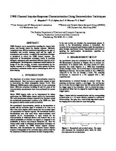
A typical impulse response measured in LOS conditions 1 m apart is shown in Figure 10 through its In-phase (a), Quadrature-phase (b) components and the amplitude (c) and power (d) profiles. The (a)

(b)

(c)

Direct Path

(d)

Reflection by the Ceiling Reflection by the Floor

Figure 10: In-phase, Quadrature-phase, Amplitude and Power Profiles, measured in LOS conditions 1 m apart; amplitude and power levels are normalized to the total root mean power and to the mean power received at 1m, respectively.

multipath components evidenced in the power-delay profile (d) have been associated to specific paths by correlating the excess delay to the path length. Figure 11 shows three exemplary power profiles of impulse responses obtained in NLOS conditions within the rooms 4185 (a), 4186 (b) and 4187 (c), measured at a transmitter-receiver distance of 4.0 m, 4.0 m and 5.3 m, respectively. The upper trace exhibits a higher signal-to-noise ratio and a “fast” time decay while the lower trace exhibits a lower signal-to-noise ratio and a “slow” time decay. In both Figure 10 and Figure 11 the amplitude and power levels have been normalized to the total root mean power and to the mean power received at 1 m, respectively.


Page 37 of 61

Figure 11: Local power profiles detected in NLOS conditions, within rooms 4185 (a), 4186 (b) and 4187 (c) , measured at a transmitter-receiver distance of 4.0 m, 4.8 m and 5.3 m, respectively, while being the transmitter at location “Tx1”; power levels are normalized to the total mean power received in LOS 1m apart.

The statistical properties of the multipath profiles in different rooms on the same floor have been investigated, which has led to a stochastic tapped delay line (STDL) model of the UWB indoor channel in the FCC compliant band 3.6-6GHz. The large and the small scale behavior of the channel have been characterized in line-of-sight (LOS) conditions by analyzing 625 responses recorded in an office room over a measurement grid (625 points with 2 cm spacing) covering 0.25 m2 and 11 impulse responses recorded in the corridor with an incremental spacing of 1m. A complete STDL model providing all the parameters and distributions to reconstruct the power/amplitude-delay profile of the channel has also been derived in nonline-of-sight (NLOS) conditions by analyzing the data collected while positioning the transmitter in one of six different locations on the corridor and moving the receiver over a finely spaced (625 points with 2 cm spacing) measurement grid within one of 16 rooms on the same floor. To characterize the UWB indoor channel, we have divided the temporal axis into delay bins having duration of 1ns, which is the width of the basic received pulse as verified by inspection of the obtained channel impulse responses. We have computed the power received in each bin to obtain the local power delay profiles (local-PDPs) for each measurement location. To derive the PDP averaged over all the locations within a room (small-scale averaged PDP), as well as to characterize Restricted and Proprietary information This controlled document is the property of IST UTRAWAVES Project. Any duplication, reproduction or transmission to unauthorized parties without the prior written permission of Ultrawaves is prohibited.

Page 38 of 61

the small-scale statistics, we have aligned the measured impulse responses setting to 0 the delay of the first arriving path. We have computed the absolute propagation delay of each local PDP as: ( 30)

τ 0 = τ Offset + (d − 1) / c

where τOffset is the delay at which the first path arrives when the antennas are 1m away in LOS conditions in a corridor environment, d is the transmitter-receiver distance (in meters) and c is the speed of light. τOffset takes into account the overall delay due to the measurement equipment and the propagation over a distance of 1m, while (d-1)/c accounts for the delay due to the propagation over the distance (d-1) m. To reduce the noise we have set the power of all the bins below a threshold to zero in the localPDPs. The noise floor, separately computed for each receiver location, is set to be 30dB below the maximum level of the local-PDP. Actually, the percent power of the small-scale averaged PDPs (SSA-PDPs) contained above this threshold is greater than 99% for all the considered cases.

3.2 The Large Scale Behaviour To characterize the large scale statistics of the channel, the dependence of the average energy on the transmitter-receiver separation have been studied and the path loss exponents in LOS and NLOS conditions have been evaluated by applying a linear fit to the values obtained by normalizing the total average power received at the each examined location (evaluated by integrating the SSA-PDP of each room over all delay bins) to the power received at the reference distance d0=1m. The total received energy experiences a shadowing around the mean energy given by the path-loss law, that can be modeled by a lognormal distribution [1] [40] [41], with standard deviation derived from experimental path loss values. Other important issues have also been investigated in this work, i.e. model parameters have been found that best fit the characteristic of the channel, such as the cluster arrival rate, the cluster decay factor and the ray decay factor, evaluated by analyzing the SSA-PDP decay with excess delay.

3.3 The Small Scale Behaviour The statistical deviations of the instantaneous normalized power levels in each bin from the average value given by the SSA-PDP have been evaluated by selecting the distribution that best fits the experimental data with a 95%-confidence interval. We have used the Chi-square test and the Kolmogorov-Smirnov test. The former selects the theoretical distribution that minimizes the meansquare error of the theoretical and empirical probability density functions. The latter selects the theoretical distribution that minimizes the absolute value of the linear error of the theoretical and empirical cumulative distribution functions. Both tests consider the most common distributions used to fit the statistics of the small-scale effects in indoor environment listed in Table 3. The statistical fits of the empirical distribution of the channel path gains can be done considering the amplitude or, equivalently, the power path gains; commonly in the literature people refer to the distribution of the amplitude path gains, such as Rayleigh or Rician, etc. If the amplitude path gains follow a given distribution p Ai ( Ai ) , the distribution associated to the power path gains Wi = Ai2

(

)

results, by a simple change of variable [42]: pWi (Wi ) = p Ai ( Wi ) 2 Wi . For the convenience of Restricted and Proprietary information This controlled document is the property of IST UTRAWAVES Project. Any duplication, reproduction or transmission to unauthorized parties without the prior written permission of Ultrawaves is prohibited.

Page 39 of 61

the reader, we have listed in Table 3 : the most common associated distributions for the amplitude and power path gains. Distributions for the Amplitude Path Gains

RAYLEIGH: p A ( A) =

RICE: p A ( A) =

A

σ2

e

A

e

σ2 −

A2

−

EXPONENTIAL: pW (W ) =

2σ 2

A2 + s 2 2σ 2

Corresponding Distributions for the Power Path Gains

I0 (

) 2

pW (W ) = A2

2 A 2 a −1 − b NAKAGAMI: p A ( A) = e Γ(a ) b a

1 2σ

2

e

−

W +s2 2σ 2

I0 ( W

e

s

σ2

1 W  GAMMA: pW (W ) =   b Γ(a )  b 

α

 A −  α −1  β 

WEIBULL: p A ( A) = αβ −α A

−

W 2σ 2

e 2σ 2 NONCENTRAL CHI-SQUARE (2 degrees of freedom):

As

σ

1

WEIBULL: pW (W ) =

), W ≥ 0

a −1

αβ −α 2

e −(W / b ) α

W

2

−1 −

e

Wα

β

2

α

LOGNORMAL: p A ( A) =

2 A 2πσ

2

e

−

( 2 ln( A ) − µ ) 2 2σ 2

LOGNORMAL: pW (W ) =

1 W 2πσ

2

e

−

(ln(W ) − µ ) 2 2σ 2

Table 3 : The most common probability density functions used to fit the empirical.


Page 40 of 61

Chapter 4

The Preliminary Channel Model

The UWB indoor channel has been characterized, based on data collected on a floor of a modern office building. The recovered impulse responses have been post-processed by best-fit procedures, to set up a statistical tapped delay line channel model. We have characterized the attenuation of the total received power due to the transmitter-receiver distance, both for LOS and for NLOS conditions, by the commonly used distance power low, adopting a lognormal distribution for the shadowing effects. A clustered structure has been observed for the average power-delay profiles, which means that rays arrive at the receiver in groups, each group having a given decay constant. The small-scale statistic of the channel has also been determined by selecting the distribution that verifies with a confidence level of 95% both the Chi-square and the Kolmogorov-Smirnov test applied to empirical data.

4.1 Large Scale Fading As already described, the path loss exponents in LOS and NLOS conditions have been extracted by linear fitting the values obtained by normalizing the total average power detected at the each receiver location to the power measured at the reference distance d0=1m. We used all the profiles measured in LOS conditions, while we selected a subset of 9x625 profiles measured in NLOS conditions, discarding the profiles having an average power below the noise floor. The scatters plots of the path loss attenuation vs. distance are shown in Figure 12, for LOS and NLOS conditions, respectively. The blue dots in subplot (a) are the attenuation values in LOS conditions, in a corridor environment. The gray stars in subplot (b) represent the attenuation values on each point of the considered measurement grids, while the colored markers are the mean attenuations evaluated over each grid. All the attenuation values are normalized to the attenuation detected 1 m apart in the Corridor, in LOS conditions and are expressed in dB.


Page 41 of 61

Figure 12: Scatter plots in LOS and NLOS conditions of the path loss attenuation vs. the logarithm of the distance (in meters). The values are normalized to the attenuation detected at 1 m distance in the Corridor, in LOS conditions.

We model the path loss of the total received power by the following distance power law for LOS and NLOS conditions, respectively:

( 31 )

 d  PL( d )[dB ] = 1.82 + 10 × 1.938 × Log 10  , LOS  d0   d  PL( d )[dB ] = −3.93 + 10 × 3.897 × Log 10  , NLOS  d0 

where PL is the mean path loss, d0 is the reference distance, and d is the transmitter-receiver distance in the intervals [1-11]m (LOS) and [5.7-8.6]m (NLOS) [39]. Due to shadowing effects statistical deviations of the total average detected power from the deterministic values in ( 31) occur, modeled by lognormal distributions having standard deviations (calculated from the experimental path loss values) σLOS=1.45 and σNLOS=2.31 for the LOS and NLOS data, respectively. The SSA-PDPs, obtained by aligning and averaging the local PDPs over the 625 realizations within each room, exhibit a clustering structure and an exponentially decay with decay constants depending on the excess delay. Energy has been detected within each delay bin at the receiver side, so a continuous model for the arrival time of rays inside each cluster has been derived. Restricted and Proprietary information This controlled document is the property of IST UTRAWAVES Project. Any duplication, reproduction or transmission to unauthorized parties without the prior written permission of Ultrawaves is prohibited.

Page 42 of 61

Three typical SSA-PDPs detected in NLOS conditions in the office environment are shown in Figure 13. The powers, normalized with respect to the total power detected at 1m distance in the corridor environment, in LOS conditions, are represented in a logarithm scale, to evidence the separation among clusters and to determine for each cluster the line that better fits the data in a least-squares sense.

Figure 13: Three typical normalized SSA-PDPs detected in NLOS conditions in the office environment (powers are expressed in a logarithm scale).

In the first curve (Figure 13a) it is shown the SSA-PDP detected within the room 4184, while being the transmitting antenna at location “Tx1” (Figure 7) in the corridor. A single dense cluster of diffuse multipath is evident, with several interspersed dominant paths. The second curve (Figure 13b) refers to measurements done within room 4186 while still being the transmitter in “Tx1”. In this case, corresponding to the situation that most frequently emerges from the experimental data, two clusters are present, having markedly different slopes. Finally, the third curve (Figure 13c) presents data collected in room 4189 with the transmitter in “Tx3”. This is the only observed case in which three clusters have been evidenced in NLOS conditions. In this room the inter-arrival time between the first and the second cluster is 16ns, while the inter-arrival time between the second and the third cluster and 25ns. Actually, each measured SSA-PDP, after being normalized as described above, can be expressed as: Restricted and Proprietary information This controlled document is the property of IST UTRAWAVES Project. Any duplication, reproduction or transmission to unauthorized parties without the prior written permission of Ultrawaves is prohibited.

Page 43 of 61

g (τ ) =

( 32 )

Nbins

∑G k =1

k

⋅ δ (t − τ k )

Nbins is the number of bins in the observation window, while G k is:

G k = Ωl ⋅ e

( 33 )

τk

−

γl

, with l ∈ {1,..,L } and

Ωl = Ω0 ⋅ e

τl

−

Γ

where L is the number of arrived clusters, γl is the decay constant of the lth cluster, τl is the excess delay of the 1st path in the lth cluster and Γ is the cluster decay constant. In the following table (Table 4) the regression lines that better fits to the logarithm of the normalized power values in a least-squares sense are reported for a subset of 9 normalized SSA-PDPs measured in NLOS conditions.

Scenario Tx1-4185 Tx1-4186 Tx1-4187 Tx3-4188 Tx3-4189 Tx1-4184 Tx4-4198 Tx5-4192 Tx2-4197

Regression lines: −  1  ⋅ τ k + ln(Ω l )  γl  1st cluster 2nd cluster -0.0654 ⋅ τl -1.1884 -0.1412 ⋅ τk - 0.6689 -0.0414 ⋅ τk - 2.1598 -0.0883 ⋅ τl -0.4067 -0.1615 ⋅ τk - 0.8600 -0.0400 ⋅ τk - 2.1887 -0.0770 ⋅ τl -2.9693 -0.0860 ⋅ τk - 2.8651 -0.0241 ⋅ τk - 4.2861 -0.0427 ⋅ τk - 2.8315 -0.0754 ⋅ τl -0.7496 -0.1649 ⋅ τk - 0.6687 -0.0976 ⋅ τk - 0.4628 -0.0163 ⋅ τk - 5.1059 -0.0186 ⋅ τk - 5.2542 -0.0049 ⋅ τk - 6.2317 -0.0033 ⋅ τk - 6.3171 Regression line: − 1 ⋅τl + ln(Ω0 ) Γ

( )

3rd cluster

-0.0362 ⋅ τk -2.8532

Table 4: Regression lines for a subset of 9 normalized SSA-PDPs measured in NLOS conditions.

From values reported in Table 4, it emerges that the cluster decay constant (Γ ) mean value is about 13ns, with a standard deviation minor than 2ns. Considering all the rooms where two or more clusters are present, the mean inter-arrival time between the first and the second cluster is 17ns (therefore the mean cluster arrival rate is Λ[1/nsec] = 0.059) with a standard deviation of about 4ns. In all examined rooms the power delay profiles completely decay within the first 100ns. By averaging results collected in rooms where two or more clusters characterize the SSA-PDP, the line that better fits in a least-squares sense the logarithm of the experimental data within the first cluster is: ( 34 )

y1= -0.1384 ⋅ τk -1.2657


Page 44 of 61

where γ1 = (1/0.1384) ≈7ns is the exponential decay constant associated to the first cluster. Considering instead rooms where just one cluster has been revealed, the line fitting data in the first cluster is: y1= -0.0172 ⋅ τk -5.1481

( 35 )

With an exponential decay γ1 = (1/0.0172) ≈58 ns. As regards the second cluster, we obtain: y2= -0.0508 ⋅ τk -2.2744

( 36 )

where γ2 = (1/0.0508) = 19,7ns is the decay constant associated to the second cluster. Finally, analyzing data collected in room 4189, while being the transmitter located in “Tx3” (Figure 13c), we derive that the line that better fits to the logarithm of the normalized power values in the third cluster is: ( 37 )

y3= -0.0362⋅ τk -2.8532

Therefore the relative decay constant is γ3 = (1/0.0362) = 27.62ns. A SSA-PDP, obtained by averaging the power delay profiles detected over a measurement grid, in LOS conditions, in the Office environment, is shown in Figure 14. The powers, normalized with respect to the total power detected at a 1m distance in the corridor environment in LOS conditions, are represented in a logarithm scale. In LOS conditions, as well as in NLOS conditions, the power delay profiles completely decay within the first 100ns, but in this case the profile exhibits a very particular behaviour along the time axis: three clusters arrive, which present almost the same shape, slope and time duration. Actually the inter-arrival time between clusters is constant and equal to 39ns; moreover the regression lines  −  1  ⋅ τ k + ln(Ω l ) chosen to characterize the time decay   γl   within each cluster of the evaluated SSA-PDP are (considering the normalized power values expressed in a logarithm scale): y1,LOS= - 0.0923 ⋅ τk – 1.0450 ( 38 )

y2,LOS= - 0.0716 ⋅ τk – 0.0397 y3,LOS= - 0.0840 ⋅ τk – 2.8154

and the exponential decay constants associated to the three clusters are, respectively: γ1,LOS = (1/0.0923) = 10.83ns, γ2,LOS = (1/0.0716) = 13.97ns, γ3,LOS = (1/0.0840) = 11.9ns. Restricted and Proprietary information This controlled document is the property of IST UTRAWAVES Project. Any duplication, reproduction or transmission to unauthorized parties without the prior written permission of Ultrawaves is prohibited.

Page 45 of 61

Finally, an exponential decay (linear if powers are expressed in a logarithm scale) can be observed between the three clusters: ( 39 )

( )

y = − 1 ⋅ τ l + ln(Ω0 ) = -0.0397 ⋅τ l − 0.1448 Γ

Figure 14: Normalized SSA-PDP evaluated in LOS conditions, in an office environment (powers are expressed in a logarithm scale).

4.2 Small Scale Fading Although the Lognormal distribution verifies the statistical tests in many bins, the distribution that satisfies both tests in most of bins is the Gamma distribution (see Table 3 : ). The a-Gamma parameter of the power path gains distribution corresponds to the m-Nakagami parameter of the amplitudes distribution, while the b-Gamma parameter can be expressed as Ω/a, where Ω is the mean of a Gamma distribution. Finally, the variance of a Gamma distribution with parameters a and b is ab2.


Page 46 of 61

On the following, the results obtained in two different scenarios are presented, in NLOS, in an office environment (Figure 15 and Figure 16; Figure 17 and Figure 18). Figure 15 and Figure 16 refer to data collected within room 4186, with the transmitting antenna at location “Tx1”, while Figure 17 and Figure 18 present results collected within room 4187, while still being the transmitting antenna at location “Tx1”. The mean values and the a-parameters (see Table 3 : ) of the Gamma distributions that best fit the channel path gains empirical distributions in each delay bin are shown, together with exemplary histograms of the empirical distribution of the power path gains. The channel path gains empirical distributions have been presented in the delay bins corresponding to the arrival times of the first ray of each cluster in the SSA-PDP. The path gains distribution has also been evaluated after being the power profile completely decayed, to the aim of outlining the differences with respect to the previous cases. In figures Figure 16 and Figure 18 below, the solid lines represent the Gamma distributions that fit the empirical histograms. The aparameters of the Gamma distributions spread in the range 1÷3 and remain roughly constant around 2 with the excess delay. Results obtained working in LOS conditions, in an office environment (within room 4186) are finally shown in Figure 19 and in Figure 20. The channel path gains empirical distributions have been analysed in the delay bins corresponding to the arrival times of the three clusters in the SSAPDP. For comparison, we have also evaluated the path gains empirical distribution when the power profile had completely decayed.


Page 47 of 61

Figure 15: Mean values and a-parameters of Gamma distributions for scenario Tx1-4186.

Figure 16: Histograms of the power path gains empirical distributions for scenario Tx1-4186. Restricted and Proprietary information This controlled document is the property of IST UTRAWAVES Project. Any duplication, reproduction or transmission to unauthorized parties without the prior written permission of Ultrawaves is prohibited.

Page 48 of 61

Figure 17: Mean values and a-parameters of Gamma distributions for scenario Tx1-4187.

Figure 18: Histograms of the power path gains empirical distributions for scenario Tx1-4187.


Page 49 of 61

Figure 19: Mean values and a-parameters of Gamma distributions in LOS conditions, office environment (room 4184).

Figure 20: Histograms of the power path gains empirical distributions in LOS conditions, office environment (room 4184). Restricted and Proprietary information This controlled document is the property of IST UTRAWAVES Project. Any duplication, reproduction or transmission to unauthorized parties without the prior written permission of Ultrawaves is prohibited.

Page 50 of 61

References [1] D. Cassioli, M. Z. Win and A. F. Molisch, “The Ultra-Wide Bandwidth Indoor Channel: From Statistical Model to Simulations,” in the IEEE Journal of Selected Areas in Commun., vol. 20, Issue: 6 , Aug. 2002, pp. 1247 –1257. [2] S. Y. Seidel and T. S. Rappaport, "914MHz Path Loss Prediction Models for Indoor Wireless Communications in Multifloored Buildings," in IEEE Trans. On Antennas and Propagation, vol. 40, n.2, Feb. 1992. [3] R. J. C. Bultitude, S. A. Mahmoud and W. A. Sullivan, "A comparison of indoor radio propagation characteristics at 910MHz and 1.75GHz," in IEEE JSAC vol.7, n.1, Jan. 1989. [4] F. Patenaude, J. Lodge and J. Y. Chouinard, "Eigen Analysis of wideband fading channel impulse responses," IEEE Trans. On Vehicular Technology, vol. 48, n. 2, Mar. 1999. [5] S. J. Howard and K. Pahlavan, "Measurement and Analysis of the indoor radio channel in the frequency domain," in IEEE Trans. On Instrumentation and measurement vol. 39, n. 5, Oct. 1990. [6] S. J. Howard and K. Pahlavan, "Autoregressive modeling of a wide-band indoor radio propagation," in IEEE Trans. On Commun., vol.40, n.9, Sept.1992. [7] H. Hashemi, "Impulse response modeling of indoor radio propagation channels," in IEEE JSAC, vol. 11, n. 7, Sept. 1993. [8] T. S. Rappaport, "Characterization of UHF multipath radio channels in factory buildings," in IEEE Trans. On Antennas and Propagation, vol. 37, n. 8, Aug. 1989. [9] T. S. Rappaport, S. Y. Seidel and K. Takamizawa, "Statistical channel impulse response models for factory and open plan building radio communication system design," in IEEE Trans. On Commun., vol. 39, n. 5, May 1991. [10] D. A. Hawbaker and T. S. Rappaport, "Indoor Wideband radio propagation measurement system at 1.3GHz and 4GHz," in IEEE Electronic Letters, vol. 26, n. 21, Oct. 1990. [11] A. A. M. Saleh and R. A. Valenzuela, "A statistical model for indoor multipath propagation," in IEEE JSAC, vol. SAC-5, n.2, Feb. 1987. [12] H. J. Zepernick and T. A. Wysocki, "Multipath channel parameters for the indoor radio at 2.4 GHz ISM band" in the Proc. of Vehicular Technology Conference, IEEE 49th , vol. 1, p. 190-193, 1999. [13] J. C. Haartsen and S. Mattisson, "Bluetooth a new low-power radio interface providing shortrange connectivity," in the IEEE Proceedings, vol. 88, n.10, Oct. 2000. [14] S. S. Ghassemzadeh, R. Jana, C. W. Rice, W. Turin and V. Tarokh, "A statistical path loss model for in-home UWB channels," in the Proc. of the IEEE Conference on Ultra Wideband Systems and Technologies, p. 59-64, 2002. [15] S. S. Ghassemzadeh, R. Jana, C. W. Rice, W. Turin and V. Tarokh, "Measurement and modeling of an ultra-wide bandwidth indoor channel," Preprint.


Page 51 of 61

[16] S. Mangold, M. Lott, D. Evans and R. Fifield, "Indoor radio channel modeling - Bridging from propagation details to simulation" in the Proc. of the ninth IEEE International Symposium on Personal, Indoor and Mobile Radio Communications, vol. 2, p. 625-629, 1998. [17] Q. H. Spencer, B. D. Jeffs, M. A. Jensen and A. L. Swindlehurst, "Modeling the statistical time and angle of arrival characteristics of an indoor multipath channel," in IEEE JSAC vol.18, n.3, March 2000. [18] M. Hamalainen, T. Patsi and V. Hovinen, "Ultra Wideband Indoor Radio Channel Measurements," Workshop in Finland. [19] V. Hovinen, M. Hamalainen and T. Patsi, "Ultra Wideband Indoor Radio Channel Models: Preliminary Results," in the Proc. of the IEEE Conf. on UWB Systems and Technol., May 2002. [20] A. F. AbouRaddy, S. M. Elnoubi and A. El-Shafei, "Wideband measurements and modeling of the indoor radio channel at 10GHz. Part I: Frequency domain analysis," in the Proc. of the XV National Radio Science Conf., Feb. 1998. [21] A. F. AbouRaddy, S. M. Elnoubi and A. El-Shafei, "Wideband measurements and modeling of the indoor radio channel at 10GHz. PartII: Time domain analysis," in the Proc. of the XV National Radio Science Conf., Feb. 1998. [22] G. Santella and E. Restuccia, "Analysis of frequency domain wide-band measurements of the indoor radio channel at 1, 5.5, 10, and 18GHz", Global Telecommunications Conference, 1996. [23] G. J. M. Janssen, P. A. Stigter and R. Prasad, "Wideband Indoor Channel Measurements and BER Analysis of Frequency Selective Multipath Channels at 2.4, 4.75 and 11.5 GHz", in IEEE Trans. On Comm., vol.44, n.10, 1996. [24] J. B. Andersen, T. S. Rappaport and S. Yoshida, “Propagation Measurements and Models for Wireless Communications Channels”, in IEEE Communications Magazine, Jan. 1995. [25] J. C. Chuang, “The effects of Time Delay Spread on Portable Radio Communications Channels with Digital Modulation”, in IEEE JSAC, vol. 5, n. 5, p. 879-889, June 1987. [26] A. Glazunov, H. Asplund and J. E. Berg, “Statistical analysis of measured short term impulse response functions of 1.88GHz radio channel in Stockholm with corresponding channel model,” in IEEE Vehic. Technol. Conference, 1999. [27] F. Ramirez-Mireles, M. Z. Win, R. A. Scholtz and M. A. Barnes, “Ultra-Wide bandwidth (UWB) Signal Propagation for Outdoor Wireless Communications,” in Proc. of IEEE Vehic. Tech. Conf. , VTC-1997, May 1997. [28] M. Z. Win, R. A. Scholtz, and M. A. Barnes, “Ultra -wide bandwidth signal propagation for indoor wireless communications,” in Proc. IEEE Int. Conf. on Commun., vol. 1, pp. 56–60, June 1997. Montréal, CANADA. [29] K. Siwiak and A. Petroff, “A Path Link Model for Ultra-Wide Band Pulse Transmissions,” in Proc. of the IEEE VTC Spring 2001, Rhodes 2001. [30] David Cheung and Cliff Prettie, “A Path Loss Comparison Between the 5 GHz UNII Band (802.11a) and the 2.4 GHz ISM Band (802.11b),” Intel Labs Internal Report, Intel Corporation, Jan. 2002 [31] P. Withington, “In-Building Propagation of Ultra-Wideband RF Signals,” in White Paper Pulson Communications. Restricted and Proprietary information This controlled document is the property of IST UTRAWAVES Project. Any duplication, reproduction or transmission to unauthorized parties without the prior written permission of Ultrawaves is prohibited.

Page 52 of 61

[32] G.J.M. Janssen and J.A.M. Vriens, “High Resolution Coherent RadioChannel Measurements Using Direct Sequence Spread Spectrum Modulation,” in Proc. of the IEEE Electrotechnical Conf. 1991, 6th Mediterranean, vol.1, pp. 720-727. [33] J. Kunisch and J. Pamp, “Measurement Results and Modeling Aspects for the UWB Radio Channel,” in the Proc. of the IEEE Conf. on UWB Systems and Technol., May 2002. [34] H. Hashemi, “The Indoor Radio Propagation Channel”, in the IEEE Proceedings, vol.81, n.7, July 1993. [35] J.Keignart and N.Daniele, “Subnanosecond UWB Channel Sounding in Frequency and Temporal Domain”, in IEEE Conference on Ultra Wideband Systems and Technologies, 2002. [36] A. Ruggieri and D. Cassioli, “Channel propagation models for indoor environments,” Ultrawaves Internal Report # W03-02-0010-R01 [37] Agilent Data Sheet: 8510C Network Analyzer [38] Agilent Application note AN 1287-3: Applying Error Correction to Network Analyzer Measurements TektroniX: 11801B Users Manual. [39] W. Ciccognani, A. Durantini and D. Cassioli, “Time Domain Propagation Measurements of the UWB Indoor Channel using PN–Sequence in the FCC–Compliant Band 3.6-6 GHz,” submitted to the Journal of Communications and Networks, July 31, 2003. [40] L. J. Greenstein, V. Erceg, Y. S. Yeh, and M. V. Clark, “A new path-gain/delay-spread propagation model for digital cellular channels,” IEEE Trans. on Veh. Tech., vol. 46, no. 2, pp. 477–485, May 1997. [41] V. Erceg, L. J. Greenstein, S. Y. Tjandra, S. R. Parkoff, A. Gupta, B. Kulic, A. A. Julius, and R. Bianchi, “An empirically based path loss model for wireless channels in suburban environments,” IEEE JSAC, vol. 17, no. 7, pp. 1205–1211, July 1999. [42] A. Papoulis. Probability, Random Variables, and Stochastic Processes. McGraw-Hill, Inc., Third Ed., 1991. [43] M. Z. Win, R. A. Scholtz, and M. A. Barnes, “Ultra -wide bandwidth signal propagation for indoor wireless communications,” in Proc. IEEE Int. Conf. on Commun., vol. 1, June 1997, pp. 56– 60.

Conclusions We have derived a statistical model of the UWB indoor channel based on the measurement data collected in the 4th floor of the modern office building where the Electronic Engineering Department of the University of Rome Tor Vergata is located. The measurement technique was based on the use of a carrier at the nominal frequency of 4.78GHz modulated by a train of short duration (0.4ns) pulses shaped by a PN-sequence. Thus the probe signal covers the band 3.6-6GHz. We have coherently demodulated the received signals and cross-correlated their In-phase and Qphase components to an opportune PN-sequence template to extract the channel impulse responses from the recorded profiles. Then we have post-processed these “recovered” impulse responses by best-fit procedures to set up a statistical tapped delay line model of the UWB indoor channel. We have modeled the path loss for LOS and NLOS conditions by the commonly used distance power law and the shadowing by lognormal distributions. The average power-delay profiles exhibit a Restricted and Proprietary information This controlled document is the property of IST UTRAWAVES Project. Any duplication, reproduction or transmission to unauthorized parties without the prior written permission of Ultrawaves is prohibited.

Page 53 of 61

clustered structure, which means that rays arrive at the receiver in groups, each having a given decay constant. We have characterized the small-scale statistics by selecting the distribution that verifies with a 95% -confidence interval both the Chi-square test and the Kolmogorov-Smirnov test applied to the experimental data. We have selected the Gamma distribution because it verifies the above-mentioned tests in most cases. The shape parameters of such Gamma distributions spread in the range of 1-3, and remain roughly constant around 2 with the excess delay.

Acknowledgments The authors wish to thank Alain Sibille, Christophe Roblin and all the people from ENSTA for providing the characterization of the EM antennas purchased for the experiments. We really appreciated their expertise in individuating the crucial points in the perspective of ultra wideband channel sounding. The authors wish to thank also the coordinators of the Ultrawaves consortium and in particular Rafi Zack, Gadi Shor and David Yaish, for the helpful discussions about the measurement set-up and techniques. Sincere thanks are addressed to the people from the Italian Ministry of Communications who make available part of the experimental setup for the Ultrawaves measurements. Finally, a special thanks is for the people from the Microwave Laboratory of the Electronic Engineering Department of the University of Rome Tor Vergata, in particular Prof. Limiti and Mr. De Dominicis, for providing part of the equipment for the Ultrawaves measurements and for their precious technical support.


Page 54 of 61

Annex I: Bicone Antenna Measurements September 2002 Source : Object : Recipient :

ENSTA measurements of a commercial bicone antenna carried out at ENSTA, at Radiolabs’ request. Mrs Dajana Cassioli (Radiolabs / Rome Tor Vergata).

The measurements were carried out with a VNA (8510C) over a bandwidth 2 – 10 GHz. The radiation patterns and gain measurements were performed in an anechoic chamber with 3 conical horns covering respectively the sub-bands : 2 – 3.1 GHz, 3.94 – 5.99 GHz and 7 – 10.7 GHz. It is worthwhile to note that our anechoic chamber is certified above 5 GHz. Therefore, several complementary measurements were carried out for the lower sub-band to check the chamber’s performance : symmetry checking by antenna reversal (side wall reflection) and far end chamber reflection by time domain measurements. However, the results for the first band have to be taken with caution, especially for the gain.

1. VSWR and input bandwidth


Page 55 of 61

2. Radiation patterns The E-plane (ϕ = 0) and H-plane (θ = 90 deg) cuts for each of the 3 sub-bands are presented in the following graphs :

2.1.

E-plane cuts

Lower sub-band : 90

90

20

120

20

120

60

10

150

10

150

30

30

5

5 180

0

210

180

330

0

210

330

300

240

300

240

60

15

15

270

270

(a) ϕ = 0 (b) ϕ = 0, “reversed” @ f (GHz) = 2.00 (magenta), 2.05 (blue), 2.55 (green), & 3.10 (black). Restricted and Proprietary information This controlled document is the property of IST UTRAWAVES Project. Any duplication, reproduction or transmission to unauthorized parties without the prior written permission of Ultrawaves is prohibited.

Page 56 of 61

The “reversed measurement” (b) was performed to check the anechoic chamber behaviour.

Medium sub-band :

90

90

20

120

20

120

60

60 15

15 10

150

10

150

30

5

5 180

0

210

330

180

0

330

210

270

270

@ f (GHz) =

300

240

300

240

30

3.94 (magenta) 4.00 (blue) 4.20 (green) 4.40 (red) 4.60 (cyan) 4.80 (black)

@ f (GHz) =



Page 57 of 61

Upper sub-band :

90

90

20

120

20

120

60

60 15

15 10

150

150

30

10 5

5

180

0

210

330

240

30

180

0

210

330

240

300

300 270

270

@ f (GHz) = 7.00 (magenta) 7.50 (blue) 8.00 (green) 8.50 (red) 8.75 (cyan) 9.00 (black)

@ f (GHz) =

9.00 (magenta) 9.50 (blue) 10.00 (green) 10.70 (red)


Page 58 of 61

2.2.

H-plane cuts

Lower sub-band : 90

20

120

60 15 10

150

30

5 180

0

330

210

300

240 270

@ f (GHz) = 2.00 (magenta), 2.05 (blue), 2.55 (green), & 3.10 (red).

Medium sub-band : 90

20

120

90

60 15

60 15

10

150

30

10

150

5

30

5

180

0

210

330

180

0

210

300

240

20

120

330

240

270

300 270




Page 59 of 61

Upper sub-band : 90

20

120

15

90

60

10

150

10

150

30

30

5

180

0

330

210

180

0

330

210

300

240

300

270

270 @ f (GHz) =

60

15

5

240

20

120


@ f (GHz) =

9.00 (magenta) 9.50 (blue) 10.00 (green) 10.70 (red)

3. Gain


Page 60 of 61

Gain (dBi) 10 9 8 7 6 5 4 3 2 1 0

2

3

4

5

6

7 f (GHz)

8

9

10

11

The (rough) estimation of the gain precision is about ±1 dB.


Page 61 of 61

UWB Channel Model Report

UWB Channel Model Report

Suggest Documents

Engine Compartment UWB Channel Model for Intra

In-vehicle UWB Channel Measurement, Model and ... - Thomas Zemen

IEEE 802.15.4a channel model - final report - CiteSeerX

UWB Radio Channel Modelling Considerations - Semantic Scholar

UWB Channel Impulse Response Characterization Using ... - CiteSeerX

Low-Sampling Rate UWB Channel ... - Infoscience - EPFL

uwb partition-dependent propagation model

UWB Channel Modeling for Wireless Body Area Networks ... - CiteSeerX

Channel division multiple access: The access solution for UWB ... - Hal

Experimental UWB Propagation Channel Path Loss and Time ...

sub-band analysis in uwb radio channel modeling - Semantic Scholar

Ultra Wideband (UWB) Transceiver Design Using Channel Phase ...

Channel Estimation in UWB channels using ... - EE, Technion

UWB On-Body Radio Channel Modeling Using Ray ... - IEEE Xplore

Channel Estimation for Wavelet Packet based UWB ... - IEEE Xplore

The UWB Channel in Medical Wireless Body Area Networks (WBANs)

UWB Channel for Wireless Body Area Networks at Hospital

Polarization Measurements in a UWB Multipath Channel - CiteSeerX

Intra-vehicle UWB MIMO Channel Capacity - Oakland University

IR-UWB Channel Capacity for Analog and Mostly Digital

UWB On-Body Radio Channel Modeling Using Ray ... - Google Sites

Channel Modeling for UWB WBAN On-Off Body Communication Link ...

Channel Capacity of Multi User TR-MIMO-UWB ... - IEEE Xplore

Frequency-Domain Channel Estimation for SC-FDE in UWB ...